The document discusses scatter diagrams, correlation, and linear regression. It defines key terms like predictor and response variables, positively and negatively associated variables, and the correlation coefficient. It also describes how to calculate the linear correlation coefficient and interpret it. The document shows an example of using least squares regression to fit a line to productivity and experience data. It provides formulas to calculate the slope and intercept of the regression line and how to make predictions with the line. However, predictions should stay within the scope of the observed data used to fit the model.

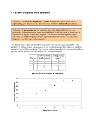
1. 4.1 Scatter Diagrams and Correlation
Definition: The response (dependent) variable is the variable whose value can be
explained by, or is determined by, the value of the predictor (independent) variable.
Definition: A scatter diagram is a graph that shows the relationship between two
quantitative variables measured on the same individual. Each individual in the data set is
represented by a point in the scatter diagram. The predictor variable is plotted on the
horizontal axis and the response variable is plotted on the vertical axis. Do not connect
the points when drawing a scatter diagram.
The data set below represents a random sample of 5 workers in a particular industry. The
productivity of each worker was measured at one point in time, and the worker was asked the
number of years of job experience. The response variable is productivity, measured in widgets
per day, and the predictor variable is experience, measured in years.
y=Productivity x=Experience
Worker (widgets/day) (years)
1 33 10
2 19 6
3 32 12
4 26 8
5 15 4
Worker Productivity vs. Experience
35
30
Productivity (widgets/day)
25
20
15
10
5
0
0 2 4 6 8 10 12 14
Experience (years)

2. Interpreting Scatter Diagrams:
Definition: Positively associated variables—when above-average values of one variable are
associated with above-average values of the corresponding variable. That is, two variables
are positively associated if, whenever the values of the predictor variable increase, the values
of the response variable also increase.
Negative associated variables—when above-average values of one variable are associated
with below-average values of the corresponding variable. That is, two variables are
negatively associated if, whenever the values of the predictor variable increase, the values of
the response variable decrease.
2

3. Correlation:
Definition: The linear correlation coefficient is a measure of the strength of linear relation
between two quantitative variables. We use the Greek letter ρ (rho) to represent the
population correlation coefficient and r to represent the sample correlation coefficient. The
formula for the sample correlation is presented below:
Sample Correlation Coefficient
 xi − x  y i − y 
∑


s x  s y 

  
r=
n −1
∑ x∑ y
∑ xy − n
r=

 x2 (∑ x )  
  y − (∑ y )
2 2


∑ i ∑
−
i 2 i
n   
i
n
   
Where: x is the sample mean of the predictor variable
sx is the sample standard deviation of the predictor variable
y is the sample mean of the response variable
sy is the sample standard deviation of the response variable
n is the number of individuals in the sample
3

4. Calculate r using the Productivity-Experience example:
y=Productivity x=Experience
Worker (widgets/day) (years) y2 x2 x* y
1 33 10
2 19 6
3 32 12
4 26 8
5 15 4
∑ y = 125 ∑ x = 40 ∑y 2
= ∑x 2
= ∑ xy =
∑ x∑ y
∑ xy − n
r=

 x2 (∑ x )  
  y − (∑ y )
2 2


∑ i ∑
−
i 2 i
n   
i
n
   
4

5. Properties of the Linear Correlation Coefficient:
1. The linear correlation coefficient is always between -1 and +1, inclusive. That is,
− 1 ≤ r ≤ +1
2. If r=+1, there is perfect positive linear relation between the two variables.
3. If r=-1, there is perfect negative linear relation between the two variables.
4. The closer r is to +1, the stronger the positive association between the two variables.
5. The closer r is to -1, the stronger the negative association between the two variables.
6. If r is close to 0, there is evidence of no linear relation between the two variables.
Because r is a measure of linear relation, a correlation coefficient close to 0 does not
imply no relation, just no linear relation.
7. The linear correlation coefficient is a unitless measure of association. So the units of
measure for x and y play no role in the interpretation of r.
How would you interpret the correlation coefficient for the Productivity-Experience example of
r=0.96?
5

6. Excel can be used to draw a scatter diagram and calculate a linear correlation coefficient.
Excel—Drawing a scatter diagram A B C
Step 1: Enter the response y=Productivity x=Experience
(dependent) variable in column B and 1 Worker (widgets/day) (years)
the predictor (independent) variable 2 1 33 10
in column C in an Excel spreadsheet. 3 2 19 6
Step 2: Select the Chart Wizard 4 3 32 12
icon. Select Chart Type of 5 4 26 8
“XY(Scatter)” and follow the 6 5 15 4
instructions.
Excel—Correlation Coefficient
Step 1: Enter raw data in columns B and C (the Excel worksheet page is shown below).
Step 2: Select Tools from the Windows menu and highlight Data Analysis. In the
Analysis Tools box, highlight “Correlation” and click OK. This brings up the Correlation
box.
Step 3: With the cursor in the “Input Range” box, highlight the data in columns B and C
(include the column headings and check the “Labels in first row” box). In the “Output
Range” box, specify a cell for the output (upper left corner of the output range). Click OK.
The correlation coefficient, r, will appear as the lower off-diagonal element in a 2x2 matrix.
A B C
y=Productivity x=Experience
1 Worker (widgets/day) (years)
2 1 33 10
3 2 19 6
4 3 32 12
5 4 26 8
6 5 15 4
7
y=Productivity x=Experience
8 (widgets/day) (years)
9 y=Productivity (widgets/day) 1
10 x=Experience (years) 0.96 1

7. 4.2 Least-Squares Regression
In this section we will learn how to fit a regression model to a scatter diagram of data. Our focus
is on regression models that produce straight (or linear) lines. Fitting a regression line involves
determining the equation for the line that “best” represents the data. Remember, a straight line
has two characteristics—(1) y-intercept and (2) slope. Thus, our goal will be to find values for
the y-intercept and the slope of the regression line.
In inferential statistics, we are concerned with estimating population parameters based on
statistics from a sample. Likewise, in regression analysis we have a population model, which
represents the true linear relation between y and x for the entire population of data, and a
statistical model, which represents the linear relation between y and x in the sample data. By
applying statistical inference, the linear relation from the sample is used as an estimate of the
unknown (true) population relation.
Population Model: yi = β0 + β1xi + εi
where yi = dependent (response) variable
xi = independent (predictor) variable
β0 and β1 are the intercept and slope parameters, respectively
εi = random error term with mean 0 and variance σε2
Note that εi accounts for factors, other than x, that affect y.
Statistical Model: yi = b0 + b1xi + ui
where yi = dependent (response) variable
xi = independent (predictor) variable
b0 and b1 are the intercept and slope statistics, respectively
ui = estimated error (or disturbance) term that accounts for factors,
other than x, that affect y
Coefficient Statistic Parameter
Intercept b0 β0
Slope b1 β1
The statistics, b0 and b1, serve as proxies (estimates) for the unknown population parameters, β0
and β1.

8. The least-squares regression coefficients (b0 and b1) are calculated based on the Least-
Squares Regression Criterion.
Definition: Least-Squares Regression Criterion
The least-squares regression line is the one that minimizes the sum of the squared
errors. It is the line that minimizes the square of the vertical distance between
ˆ
observed values of y and those predicted by the line, y (read “y-hat”). We represent
this as
Minimize Σ (errors2)
Application of the Least-Squares Regression Criterion produces the Normal Equations shown
below:
(1) b0 n + b1Σx = Σy
(2) b0Σx + b1Σx2 = Σxy
These equations can be solved to find formulas for b0 and b1 (the solution is done in reverse
order).
b1 =
∑ xy − n x y
∑ x − n(x)
2 2
b0 = y − b1 x
The final least-squares regression equation is written as: y = b0 + b1 x + u
8

9. Example—Application of Least-Squares Regression for Productivity-Experience Data
y=Productivity x=Experience
Worker (widgets/day) (years) x2 x* y
1 33 10 100 330
2 19 6 36 114
3 32 12 144 384
4 26 8 64 208
5 15 4 16 60
Σy=125 Σx=40 Σx2=360 Σxy=1,096
y = 25 x=8
Calculate the slope coefficient (b1) and the intercept coefficient (b0) using the least-squares
formulas:
Alternative way to calculate b1: If you have already calculated r,
b1 =
∑ xy − n x y
=
sy
b1 can be found using the formula b1 = r ∗ , where sy and sx are,
∑ x 2 − n(x) 2 sx
respectively, the standard deviations of the observations in the y-
b0 = y − b1 x = sample and the x-sample (see pp. 198, text).
The estimated least-squares regression equation is written as: y = ___ + ___ x + u
Interpretation of the estimated regression coefficients:
b0=____: ________________________________________________________
________________________________________________________________
Scope of the Model
The y-intercept, or b0, will have meaning only if the following two conditions are met:
(1) A value of 0 for the independent (predictor) variable makes sense;
(2) There are observed values of the independent variable near 0.
The second condition is particularly important because statisticians do not use the
regression model to make predictions outside the scope of the model (more on this
later when we discuss using the regression model to predict).
b1=___ (Remember the slope equals the change in y divided by the change in x,
∆y
i.e., b1 = .)
∆x
________________________________________________________________
________________________________________________________________
9

10. Prediction: The estimated least-squares regression equation can be used for prediction by
setting u=0 in the Statistical Model:
y = b0 + b1 x + u
y = b0 + b1 x + 0
ˆ Note: When u is set to 0, a hat is put on the y-variable.
y = b0 + b1 x
ˆ
ˆ
where y is the predicted value of y.
y = b0 + b1 x
ˆ
ˆ
y
x
Productivity-Experience Example: y = 5.8 + 2.4 x
ˆ
(1) Predict worker productivity for a worker with 7 years of experience.
(2) Predict worker productivity for a worker with 20 years of experience.
10

11. Scope of the Regression Model
Statisticians do not use the regression model to make predictions outside the scope of the
model, i.e., they do not use the regression model to make predictions for values of the
independent (predictor) variable that are much larger or smaller than those observed in the
dataset. This rule is followed because we are not certain of the behavior of the line outside
the range of the dataset used to estimate the regression model.
For example, it is not appropriate to use the line to predict the productivity of a worker with 20
years of experience. The highest value of the independent variable (in the dataset used to
estimate the regression model) is 12 years of experience and we cannot be certain that the linear
regression line will continue out to 20 years of experience. It is likely at high levels of
experience that productivity will level off as shown in the figure below.
Worker Productivity vs. Experience
45
40
Productivity (widgets/day)
35
30
25
20
15
10
5
0
0 5 10 15 20
Experience (years)
11

12. Accuracy of Predictions from the Least-Squares Regression Model:
Are the predictions from a regression model perfectly accurate?—The answer is NO. Let’s
examine how we predict with a regression model and why the predictions are usually not
perfectly accurate. First, the prediction from a regression model is represented by the equation
y = b0 + b1 x
ˆ
The statistical regression model is written as
y = b0 + b1 x + u
.
y = y +u
ˆ
The inaccuracy (or error) of a prediction is represented by u = y − y . The term “u” is referred to
ˆ
as an error term that represents all the factors, other than x, that account for (or explain) y. The
error term, u, is represented as the vertical distance between the observed value of y and the
predicted value of y, as shown in the graph below.
y = b0 + b1 x
ˆ
yi
ui = yi − yi
ˆ
ˆ
yi
xi
To get a better understanding of the error term, let’s calculate an error for the Productivity-
Experience example. Take the 4th worker with x=8 years of experience, and calculate the
worker’s predicted productivity: y 4 = 5.8 + 2.4(8) = 25 widgets / day . The actual productivity of
ˆ
th
the 4 worker was 26 widgets/day. The error in this case is u4=26-25=1 widget/day. The error is
represented in the graph below.
y = 5 .8 + 2 .4 x
ˆ
y 4 = 26
u 4 = ( y 4 − y 4 ) = (26 − 25) = 1
ˆ
y 4 = 25
ˆ
x4=8

13. Why do errors occur when making predictions?
Let’s think about why our prediction of productivity for the 4th worker was inaccurate. That is,
why did the 4th worker produce 26 widgets/day when the regression line predicted that he would
produce 25 widgets/day? Remember that y = 25 represents the productivity of the “average
ˆ
worker” with 8 years experience. The u, or the difference between 26 and 25, is due to factors,
other than x, that account for y. For example, the 4th worker could work harder than the average
worker. Or, the 4th worker could have more innate talent, or have many other characteristics—
that are different from those of the average worker—that account for the higher productivity,
In short, the 4th worker’s productivity includes two components: (1) his predicted productivity
based on years of experience, and (2) an adjustment in productivity (which can be positive or
negative) that is due to the particular “other” characteristics of the 4th worker such as work ethic,
ability, etc. The sum total of the two components account for the 4th worker’s total productivity,
i.e.,
y4 = y4 + u4
ˆ
26 = 25 + 1
In the application of the regression model to real-world, scientific data, there will always be
positive and negative u’s that account for unknown factors, other than x, that explain the y
variable. This is true for any type of scientific relation which involves a complicated process.
Only when scientists know everything, will the u’s go away…and that is a long way, or
infinitely, out into the future.
13

14. How well does the regression line fit the data?
Two measures are widely used to measure the fit of a regression line—(1) coefficient of
determination, and (2) standard error of the estimate. We will discuss each in turn.
Coefficient of Determination:
The coefficient of determination provides a quantitative measure of how well the regression line
fits the scatter plot. The coefficient of determination measures the strength of relation that exists
between two variables.
Definition: The coefficient of determination, R2, measures the proportion of the total
variation in the dependent (response) variable that is explained by the least-squares regression
line.
R2 is a number between 0 and 1, inclusive, i.e., 0 ≤ R 2 ≤ 1 . If R2 = 0, the regression line has
no explanatory power; if R2 = 1, the regression line explains 100% of the variation in the
dependent variable.
To understand the coefficient of determination, we need to understand three types of deviation.
(1) Total deviation = y − y
(2) Explained deviation = y − y
ˆ
(3) Unexplained deviation = y − y
ˆ
From the figure above notice that total deviation is the sum of the explained deviation and the
unexplained deviation:
Total deviation = Explained deviation + Unexplained deviation
y− y y− y
ˆ y− yˆ
14

15. In statistics we are generally concerned with squared deviations…Remember that variance in Ch.
3 was defined as the average of the squared deviations from the mean. Likewise, here we are
concerned with squared deviations, which are referred to as variation. Although beyond the
scope of this course, it can be shown that there are three sources of variation:
(1) total variation, ∑ ( y − y ) 2
(2) explained variation,∑ ( y − y)
ˆ 2
(3) unexplained variation, ∑ ( y − y )
ˆ 2
Furthermore, total variation is equal to the sum of explained variation and unexplained variation,
i.e.,
Total variation = Explained variation + Unexplained variation
If we divide this equation by total variation, we get
exp lained var iation un exp lained var iation
1= +
total var iation total var iation
Using algebra we can solve for R2:
exp lained var iation un exp lained var iation
R2 = = 1−
total var iation total var iation
Calculate R2 based on the correlation coefficient, r: This approach involves first calculating
the correlation coefficient and then squaring r to find R2. For the Productivity-Experience
example, we found r=0.96, and therefore, R2=(0.96)2=0.92.
An R2 value of 0.92 says that 92% of the variation in productivity (y) is explained by the linear
relation with experience (x). This leaves 8% of the variation in worker productivity left to be
explained by other factors (not x) such as work ethic, ability, health condition, etc.
15

16. Relating R2 to Scatter Diagrams:
The coefficients of determination (R2’s) for the three datasets are: 1.0, 0.947, and 0.094,
respectively.
16

17. Standard Error of the Estimate:
The variance of the error terms (εi) from the population regression model is represented by σε2,
which is a population parameter. Since a population parameter is unknown to a practicing
statistician, it must be estimated using a sample statistic. In this case, the standard error of the
estimate, se, serves as the statistic used to estimate σε. The standard error of the estimate is
found using the formula:
∑(y − yi ) 2 ∑u ∑ error
2 2
ˆ
se = = =
i i
n−2 n−2 n−2
Remember that y i = observed value of y for the ith individual
ˆ
y i = predicted value of y for the ith individual
u i = y i − y i or prediction error for the ith individual
ˆ
The standard error of the estimate measures the standard deviation of the scatter points about the
least-squares regression line.
To develop a better understanding of the standard error of the estimate, let’s calculate se for the
Productivity-Experience example. Carry out the calculations below.
Y=Productivity X=Experience
Worker (widgets/day) (years) ˆ
y ui = yi − yi
ˆ ui
2
1 33 10
2 19 6
3 32 12
4 26 8
5 15 4
Σui Σui2=
17

18. Worker Productivity vs. Experience
40
35
30
Productivity (widgets/day)
25
20
15
10
5
0
0 2 4 6 8 10 12 14
Experience (years)
Σui = 0: The sum of the vertical distance the points are off of the regression line is 0. That is,
the sum of the 2 red segments (positive errors) is exactly equal to the sum of the 3 blue segments
(i.e., the absolute value of the blue errors).
Σui2 is minimized by Least-Squares Regression Criterion: The least-squares regression line
produces the minimum sum of squared deviations of any possible linear line. That is, if you
were to draw any other line (with a different b0 and b1 than that of the least-squares line) the sum
of the squared deviations from the line would be greater than from the least-squares regression
line. See “Least-Squares Criterion Revisited,” p. 198.
18

19. How do you interpret the standard error of the estimate? At one extreme is the case where
se=0. In this situation, all the scatter points in the scatter diagram fall on a linear line and there is
no error in any prediction.
se = 0
y
x
In real-world situations, there generally are errors in the predictions and the scatter points in the
scatter diagram fall off of the least-squares regression line. The more scattered the points are
about the regression line, the higher the se. For example, the scatter diagram to the right has the
highest se.
se = small value > 0 se = large value
y y
x x
19

20. Hypothesis Test Regarding the Slope Coefficient, β1.
Assumptions:
• A random sample is drawn.
• The error terms are normally distributed with mean 0 and constant variance σε2.
Step 1: A claim is made regarding the linear relation between a response (dependent) variable,
y, and a predictor (independent) variable, x. The null hypothesis is most often specified as no
relation between y and x, i.e., β1=0. The hypotheses can be structured in one of three ways.
Two-Tailed Left-Tailed Right-Tailed
H 0: β 1 = 0 H 0: β 1 = 0 H 0: β 1 = 0
H 1: β 1 ≠ 0 H 1: β 1 < 0 H 1: β 1 > 0
β1 < 0 or β1 > 0
Step 2: Choose a significance level, α. The level of significance is used to determine the critical
t-value, with (n-2) degrees of freedom. The rejection (critical) region is the set of all values of
the test statistic (from step 3 below) such that the null hypothesis is rejected.
b1 − β 1
Step 3: Compute the test statistic: t= , which follows Student’s t-distribution with
s b1
se
df=n-2. The estimated standard deviation of b1 is s b1 = where se is the standard
∑ (x )
2
i −x
error of the estimate.
Step 4: Draw a conclusion:
• Compare the calculated t-value (or test statistic) to the critical t-value and state whether
or not H0 is rejected at the specified α.
Two-Tailed Left-Tailed Right-Tailed
If t < −t α or t > t α
2 2 If t < −tα reject If t > tα reject
reject the null hypothesis the null hypothesis. the null hypothesis.
• Interpret the conclusion in the context of the problem
20

21. Hypothesis Test Regarding the Slope Coefficient, β1.
Problem: A labor economist would like to measure the relation between the productivity of
workers and the number of years of experience of the workers. A random sample of 5 workers is
chosen. A random work day is chosen and the productivity of each worker is measured and
recorded. Work experience (in years) is taken from each worker. Carry out a hypothesis test of
the relevant null hypothesis at the 5% significance level. Show all of your calculations and
justify your conclusion.
Step 1: H0: β1 = 0 (No relation exists between worker productivity and experience.)
H1: β1 ≠ 0 (A positive or negative relation exists between productivity and experience.)
Step 2: Select α = 0.05 and find the critical value of t (df=5-2=3).
Step 3: Draw a random sample of n=5 workers and collect data on each worker’s productivity
and experience. Calculate the standard deviation of b1, sb1 , and the test statistic, t.
y=Productivity x=Experience
Worker (widgets/day) (years) (b1 − β1 ) (2.4 − 0) 2 .4
t= = = = 5.93
1 33 10 s b1 0.405 0.405
2 19 6
3 32 12 se 2.56
4 26 8 where s b1 = = = 0.405
∑ (x )
2
5 15 4 −x 40
i
Step 4: Conclusion—Because the calculated t = 5.93 is greater than the critical t = 3.182 (and in
the rejection region), reject H0 at the 0.05 significance level. A significant positive relation
exists between productivity and experience.
21

22. Excel—Estimating a linear regression model
Step 1: Enter raw data in columns B and C (the Excel worksheet page is shown below).
Step 2: Select Tools from the Windows menu and highlight Data Analysis. In the Analysis
Tools box, highlight “Regression” and click OK. This brings up the Regression box.
Step 3: With the cursor in the “Input Y Range” box, highlight the data in column B
(including the column heading at the top of the column). Move the cursor to the “Input X
Range” box and highlight the data in column C. Check the “Labels” box.
Step 4: Under Output Options, move the cursor to the “Output Range” box and specify a cell
for the output (upper left corner of the output range). Click OK and the regression output
results will appear as shown below.
A B C D E
x=Experience
1 Worker y=Productivity (widgets/day) (years)
2 1 33 10
3 2 19 6
4 3 32 12
5 4 26 8
6 5 15 4
7
8 SUMMARY OUTPUT
9
10 Regression Statistics
11 Multiple R 0.96
12 R Square 0.9216
13 Adjusted R Square 0.895466667
14 Standard Error 2.556038602
15 Observations 5
16
17 ANOVA
18 df SS MS F Signif F
19 Regression 1 230.4 230.4 35.26531 0.009546
20 Residual 3 19.6 6.533333
21 Total 4 250
22
23 Coefficients Standard Error t Stat P-value
24 Intercept (b0) 5.8 3.42928564 1.691314 0.189355
25 x=Experience (b1) 2.4 sb1=0.40414518 5.93846 0.009546

23. CHAPTER 4 Describing the Relation between Two Variables
 xi − x  y i − y 
∑





 s x  s y 
• Correlation Coefficient: r =
n −1
∑ x∑ y
∑ xy − n
r=

 x2 (∑ x )  
  y − (∑ y )
2 2


∑ i ∑
−
i 2 i
n   
i
n
   
• The equation of the least-squares regression line is
sy
y = b0 + b1 x where y is the predicted value, b1 = r
ˆ ˆ
sx
is the slope, and b0 = y − b1 x is the intercept.
• Residual = observed y – predicted y = y − y .
ˆ
• Coefficient of Determination: R2 = the percent of total
variation in the response variable that is explained by the
least-squares regression line.
• R2=r2 for the least-squares regression model.
• Least-Squares Regression Normal Equations:
(1) b0 n + b1Σx = Σy
(2) b0Σx + b1Σx2 = Σxy
• Solution of normal equations for b0 and b1:
b1 =
∑ xy − n x y
∑ x 2 − n(x) 2
b0 = y − b1 x
• The final least-squares regression equation is written as:
y = b0 + b1 x + u
23