An econometric analysis of the relationship between gdp growth rate and exchange rate in ghana
•
0 likes•933 views

International peer-reviewed academic journals call for papers, http://www.iiste.org/Journals

Recommended
Recommended
More Related Content
What's hot
What's hot (20)
Viewers also liked
Viewers also liked (9)
Similar to An econometric analysis of the relationship between gdp growth rate and exchange rate in ghana
Similar to An econometric analysis of the relationship between gdp growth rate and exchange rate in ghana (20)
More from Alexander Decker
More from Alexander Decker (20)
Recently uploaded
Recently uploaded (20)
An econometric analysis of the relationship between gdp growth rate and exchange rate in ghana
- 1. Journal of Economics and Sustainable Development www.iiste.org ISSN 2222-1700 (Paper) ISSN 2222-2855 (Online) Vol.4, No.9, 2013 1 An Econometric Analysis of the Relationship between Gdp Growth Rate and Exchange Rate in Ghana Prudence Attah-Obeng1 Patrick Enu2* F. Osei-Gyimah3 C.D.K. Opoku4 1. University of Ottawa, Canada. 2111-170 Lees Avenue , Ottawa ON, K1S5G5 +447572674481 2. Economics Department, Methodist University College Ghana. P.O. Box DC 940, Dansoman, Accra, Ghana. +233242255846 3. Economics Department, Methodist University College Ghana. P.O. Box DC 940, Dansoman, Accra, Ghana +233208215615 4. Economics Department, Methodist University College Ghana. P.O. Box DC 940, Dansoman, Accra, Ghana +233546632553 *Email of the corresponding author: penu@mucg.edu.gh Abstract This study attempts to examine the relationship between GDP growth rate and exchange rate in Ghana from the period 1980 to 2012. The paper employs the graphing of the scatter diagram for the two variables which are GDP growth rate and exchange rate, establishes the correlation between GDP growth rate and exchange rate using the Pearson’s Product Moment Correlation Coefficient (PPMC) and finally estimates the simple linear regression using OLS. Further tests were performed to test for the presence of autocorrelation, heteroscedasticity and multicollinearity. Autocorrelation and heteroscedasticity were found to be absent. From our analyses, we strongly conclude that there is a positive relationship between GDP growth rate and exchange rate in Ghana which confirms to the theory that undervaluation (high exchange rate) stimulates economic growth in the short run. Therefore, policy makers should stabilise monetary and fiscal policies in the long run. Keywords: GDP growth rate, Exchange rate, Ordinary Least Squares 1. Introduction This study attempts to examine the relationship between GDP growth rate and exchange rate in Ghana from the period 1980 to 2012. The paper employs the graphing of the scatter diagram for the two variables which are GDP growth rate and exchange rate, establishes the correlation between them using the Pearson’s product moment correlation coefficient and finally estimates the simple linear regression using the ordinary least squares estimation technique. According to Mishkin (2007) exchange rate is the price of one currency in terms of another. It affects an economy and its standard of living. The reason is that for instance, when the Ghanaian cedi becomes more valuable relative to foreign currencies, foreign goods become cheaper for Ghanaians and Ghana goods become more expensive to foreigners. There are two main kinds of exchange rate. They are spot transactions (it is the exchange rate for the spot) and forward transaction (it is the exchange rate for the forward transaction). When a currency increases in value, it is called appreciation and when it decreases in value, it is called depreciation. Exchange rates are important because they affect the relative price of domestic and foreign goods (Mishkin, 2007). Exchange rate can be determined by the interaction between demand and supply in the foreign exchange market. Such supply and demand conditions are determined by whether the country’s basic balance of payments is in surplus or deficit (Mishkin, 2007). And also, in the long term, through the theory of purchasing power parity (PPP), which states that exchange rates between two currencies will adjust to reflect changes in the price level of the two countries. The long run exchange rate is affected by relative price levels, tariffs and quotas, preferences for domestic versus foreign goods and productivity. Domestic price level and import demand all have an inverse relationship with exchange rate, while trade barriers, export demand and productivity all have a positive relationship with exchange rate (Mishkin, 2007). Exchange rates can be fixed at a predetermined level (fixed exchange rate) or they can be flexible to reflect changes in demand (floating exchange rate). This can affect national output either negatively or positively. The reason is due to the fact that exchange rates impact on prices. That is Ghana’s net exports fall when the Ghanaian cedi goes up in value as compared to other foreign countries. This will cause aggregate demand to decrease. A drop in the value of the Ghanaian cedi will have the opposite effect, that is, net exports rise, thereby increasing aggregate demand. The relationship between GDP growth rate and exchange rate has mixed results. It could be positive, negative or no relation at all as seen from above. For instance, according to Rodrik (1998) in his work “the real exchange rate and economic growth: theory and evidence”, undervaluation (high exchange rate) stimulates the growth of an economy. That is, there is a positive relationship between exchange rate and the GDP growth rate and that this is true particularly for developing countries, suggesting that tradable goods suffer disproportionately from the
- 2. Journal of Economics and Sustainable Development www.iiste.org ISSN 2222-1700 (Paper) ISSN 2222-2855 (Online) Vol.4, No.9, 2013 2 distortions that keep poor countries from converging. The countries used in his work as evidence were China, India, South Korea, Taiwan, Uganda, and Tanzania. McPherson et al (1998) researched on “Exchange Rates and Economic Growth in Kenya: An Econometric Analysis”. Their objective was to determine the relationship between exchange rate and economic growth in Kenya based on the data for the period 1970 to 1996. They analysed the possible direct and indirect relationship between the real and nominal exchange rates and GDP growth. They derived these relationships in three ways: within the context of a fully specified (but small) macroeconomic model, as a single-equation instrumental variable estimation, and as a vector auto regression model. The estimation results from the three different settings showed that there was no evidence of a strong direct relationship between changes in the exchange rate and GDP growth. Hadad et al (2010) worked on “Can real exchange rate undervaluation boost exports and growth in developing countries?” They concluded affirmatively, but not for long. Current discussions over the value of China’s currency demonstrate the controversy that exchange-rate policy is capable of igniting. This column suggests that while a managed real undervaluation can enhance domestic competitiveness, it is difficult to sustain in the post- crisis environment – both economically and politically. It says that a real undervaluation works only for low- income countries, and only in the medium term. Chen (2012) researched on “Real exchange rate and economic growth: Evidence from Chinese provincial data (1992-2008)”. His paper studied the role of the real exchange rate on economic growth and in the convergence of growth rates among provinces in China. Using data from 28 Chinese provinces for the period 1992-2008 together with dynamic panel data estimation, he found conditional convergence among coastal provinces and also among inland provinces. The results reported here confirm the positive effect of real exchange rate appreciation on economic growth in the provinces. Tarawalie (2010) researched on “Real exchange rate behaviour and economic growth: evidence from Sierra Leone”. The main focus of this paper was to examine the impact of the real effective exchange rate on economic growth in Sierra Leone. First, an analytical framework was developed to identify the determinants of the real effective exchange rate. Using quarterly data and employing recent econometric techniques, the relationship between the effective exchange rate and economic growth was then investigated. A bivariate Granger causality test was also employed as part of the methodology to examine the causal relationship between the real exchange rate and economic growth. The empirical results suggested that the real effective exchange rate correlates positively with economic growth, with a statistically significant coefficient. The results also indicated that monetary policy was relatively more effective than fiscal policy in the long run, and evidence of the real effective exchange rate causing economic growth was profound. In addition, the results showed that terms of trade, exchange rate devaluation, investment to GDP ratio and an excessive supply of domestic credit were the main determinants of the real exchange rate in Sierra Leone. Mohammed (2009) compared the economic track records of two different exchange rate regimes: the “Fixed Exchange Rate” and the “Free Floating Exchange Rate System”, in maintaining economic performance. The paper considered relationships between exchange rate and inflation and between exchange rate and GDP in Bangladesh. The experiences of moving away from a currency board system to floating regime since 2003 offers a lesson worthy of attention from the point of view of efficiency of “Floating Rate System” in least developed countries. Floating exchange rate regime in Bangladesh contrasts with its neighbor’s currency board system. Experiences in Bangladesh and abroad showed that all that a government needs in this regard is to maintain confidence in the currency, secure the currency's strength and ensure its full convertibility. As long as this is backed by sufficient reserve of the foreign exchanges and there is firm political and economic will, adoption of a successful free exchange rate regime is possible. From the above discussions, we could infer that the link between GDP growth rate and exchange rate has mixed results. What is the situation in Ghana? Ghana is an import inelastic country and issues concerning exchange rate and economic expansion cannot be overruled, hence, the need for this study. 2. Objective Our main objective of this study is to examine the relationship between GDP growth rate and exchange rate in Ghana from the period 1980 to 2012. 3. Hypothesis H0: There is no positive relationship between GDP growth rate and exchange rate in Ghana. H1: There is a positive relationship between GDP growth rate and exchange rate in Ghana. 4. Materials and Methods In this work, we will employ three basic methods. They are the scatter diagram approach, correlation analysis
- 3. Journal of Economics and Sustainable Development www.iiste.org ISSN 2222-1700 (Paper) ISSN 2222-2855 (Online) Vol.4, No.9, 2013 3 and simple linear regression analysis. The Scatter diagram is a figure in which each pair of independent – dependent observation is plotted as a point in the x-y plane. It is the first thing one needs to do in regression analysis. Its purpose is to determine by inspection, if there exist an appropriate linear relationship between the dependent variable and the independent variable. In a scatter diagram analysis, one variable is plotted on the x – axis (the independent variable) and the other variable is plotted on the y-axis (the dependent variable) (Mendehhall et al., 1989; Oakshott, 2006). In this study, we plot the exchange rate variable on the x-axis and the GDP growth rate on the y-axis. This is because we believe that the exchange rate variable influences GDP growth rates .Scatter diagram does not actually measure the strength of the association, hence, the need for correlation analysis (Mendehhall et al., 1989; Oakshott, 2006). The correlation analysis shows the strength of the relationship between two variables. Correlation tells us two things: it tells us the direction and the degree of the association between the two variables. Correlation analysis also evaluates cause/effect of one variable against the other. Correlation can be calculated by using the Spearman’s Rank- Order correlation coefficient and the Pearson’s Product moment correlation coefficient. Both give a value between -1 and +1. When the correlation value is -1, it indicates perfect negative correlation and if +1, indicates a perfect positive correlation and zero, indicates no evidences of correlation (Mendehhall et al., 1989; Oakshott, 2006). In this study, however, we employ the Pearson’s Product moment correlation coefficient (PPMC) which is given as: 2 2 2 2 n ( xy) - ( x) ( y) r = [n( x ) - ( x) ][n( y ) - ( y) ] ∑ ∑ ∑ ∑ ∑ ∑ ∑ where x = exchange rate, y = GDP growth rate and n = the number of data pairs. Excel will be used to estimate the value of the PPMC. In addition, we will have to establish how significant the correlation coefficient is. This will enable us to ascertain how meaningful the regression line is.. Here, we will employ the formula for the test of the correlation coefficient which is given as 2 n - 2 t = r 1 - r with degrees of freedom equal n – 2 to test for the statistical significance of the r. We first of all state our hypotheses which are 0H : = 0ρ and 1H : 0ρ ≠ . We will then find the critical value of t which is given by the formula α , n-2 2 t at a given significance level (say 5%).We compute the test value with the formula given. We then compare the computed test value with that of the critical value. If the test value is greater than the critical value, then we will conclude that there is a significant relationship between GDP growth rate and exchange or otherwise (Mendehhall et al., 1989; Oakshott, 2006,). The Pearson correlation coefficient does not measure cause and effect, hence, simple linear regression analysis is required (Mendehhall et al., 1989; Oakshott, 2006). The simple linear regression analysis is also used in this study. Regression analysis studies the causal relationship between one economic variable to be explained (the dependent variable) and one or more independent variables. It helps us to see the trend and make predictions outside or within a given data. Regression gives the cause and effect of one variable on the other (Mendehhall et al., 1989; Oakshott, 2006). Due to the linear relationship between GDP growth rate and exchange rate, our model specification is stated of the form: t 0 1 t tGDPGR = b + b EXR + U , where; GDPGRt is the dependent variable and denotes GDP growth rate at time t. EXRt is the independent variable and denotes exchange rate at time t. b0 and b1 denote the parameters or constants, b0 is the intercept and b1 is the slope of the GDP growth equation. Ut denotes the error term normally distributed with a zero mean and a constant variance. The values of b0 and b1 will be obtained by using the ordinary least squares estimation technique by the help of an econometric package called gretle. This is because this estimation technique is widely used in regression analysis for estimating the parameter values in a regression equation. The value of the R2 is used to determine how strong or weak the regression equation is. If R2 value lies between 0.8 and 1, then we can conclude that the regression equation is strong. However, if the value of the R2 lies between 0 and 0.5, then we can say that the regression equation is a weak one. In addition, the value of the R2 is used to determine by how much the change in the independent variable(s) explain the changes in the dependent variable, called the explained variation. The unexplained variation is given as (1 – R2 ) which takes care of the other factors that are not included in the regression equation (Shim et al., 1995).
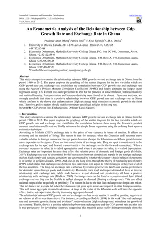
- 4. Journal of Economics and Sustainable Development www.iiste.org ISSN 2222-1700 (Paper) ISSN 2222-2855 (Online) Vol.4, No.9, 2013 4 The value of the F statistic is used to ascertain the overall significance of the GDP growth rate equation. We compare the value of the F statistic ( 2 2 R kF = (1 - R ) [n - (k + 1)] ) with the value of the critical value of F ( , k - 1, n - kFα where k = number of parameters and n = number of observations) at a given significance level usually 5% (Shim et al., 1995). If the value of the F statistic is greater than the value of the F critical, then the overall GDP growth rate equation is statistically significant or otherwise. The statistical significance of the parameters will be established. In testing for the statistical significance of the parameters, we use the rule of thumb and the t-test. The rule of thumb states that for a parameter to be statistically significant, the absolute value of the t-statistic should be greater than or equal to two. Using the t-test, the t- critical value is compared with the t-statistic at a given significance level (5%). If the t-statistic is greater than the t-critical value, then, the parameter in question is statistically significant. If otherwise, then, the parameter is not statistically significant. The t-critical value is given by tα/2,n-k (n = number of observations and k is the number of parameters) where n-k is the degree of freedom and α is the level of significance . The critical value of t is obtained from the t distribution table (Koutsoyiannis, 2006; Gujarati et al., 2009; Wooldridge, 2006). There are three major problems which affect regression results. These problems are heteroscedasticity, autocorrelation and multicollinearity (Salvatore, 2002). There are several methods we can use in testing for the presence of these problems. In our study, in testing for the presence of heteroscedasticity, we employed the Spearman Rank Correlation. Here, we find the error terms which is defined as t t t ˆe = (Y - Y ) where Yt is the actual values of the GDP growth rate and t ˆY is the estimated values of the GDP growth rate. The estimate for each year is given by substituting the value of the exchange rate into the given GDP growth rate regression equation model. We then find the error term for each year, obtain their absolute values, rank them in ascending order with the explained variable (exchange rate). We obtain for each pair the difference between the rankings. We then square the differences and sum. We substitute the sum of the differences square into the spearman’s rank correlation coefficient formula which is given as 2 2 6 d r = 1 - n(n - 1) ∑ . The decision rule is that very low rank correlation coefficient indicates the absence of heteroscedasticity. In other words, high values of r indicate the presence of heteroscedasticity (that is a coefficient of 0.5 and above in absolute terms suggest the existence of heteroscedasticity) (Koutsoyiannis, 2006). Also, Durbin-Watson test was used to test for the presence of autocorrelation. Our hypothesis here is stated as H0: no autocorrelation, against H1: there is autocorrelation. The formula for finding the Durbin-Watson test statistic is given as 2 t t-1 2 t (e - e ) d = e ∑ ∑ where et is the error term and e t-1 is the lagged error term. Roughly speaking, if the DW lies between 1.5 and 2.5, it is an indication of no autocorrelation or otherwise (Shim et al., 1995). Multicollinearity is not a problem in our study because there is only one independent variable (Koutsoyiannis, 2006; Gujarati et al., 2009; Wooldridge, 2006). The data used for this study was secondary data collected from the Ghana Statistical service (GSS). 5. Results and Discussion 5.1 Scatter Diagram Approach The scatter diagram of the GDP growth rate and the exchange rate is given at the notes section. From the scatter diagram it can be seen that there exist a positive linear relationship between GDP growth rate and the exchange rate. That is, GDPG = 4.23 + 2.33EXR, where +2.33 is the slope of the equation and 4.23 is the intercept of the diagram. Therefore, from the scatter diagram approach, there is a positive linear relationship between GDP growth rate and exchange rate in Ghana. There is no evidence of non-linearity in the data. 5.2 Correlation Analysis 5.2.1 Pearson’s Product Moment Correlation Coefficient [PPMC] The correlation between the GDP growth rate and exchange rate is 0.54847882. From the correlation given, we can infer that GDP growth rate and exchange rate are positively related. This implies that as exchange rate increases, GDP growth rate also increases. However, the degree of the association between GDP growth rate and
- 5. Journal of Economics and Sustainable Development www.iiste.org ISSN 2222-1700 (Paper) ISSN 2222-2855 (Online) Vol.4, No.9, 2013 5 exchange rate is a moderate one. Also, there is a significant relationship between GDP growth rate and exchange rate since the test value (3.6523) is greater than the critical value of t (2.04). Therefore, the result from the PPMC also confirms that there is a significant positive linear relationship between GDP growth rate and exchange rate in Ghana. 5.3 Simple Linear Regression 5.3.1 DW and R2 The values of the DW and R2 are 1.82698 and 0.300829 respectively. The value of the Durbin-Watson is greater than the value of the R2 . That is 1.82698 > 0.300829. This means that the regression results are sensible and the model can be accepted. 5.3.2 Testing for the presence of Heteroscedasticity using the Spearman’s Rank Correlation Coefficient To test for heteroscedasticity, using spearman’s rank correlation, we obtained r = -0.0296, which is a very low rank correlation. This indicates the absence of heteroscedasticity. 5.3.3 Testing for the presence of autocorrelation using the Durbin – Watson test Using the Durbin –Watson test formula, we obtain 1.82698. Based on the decision rule (n =33 and k = 1, from the Durbin-Watson table, dL = 1.17 and dU= 1.29) we accept H0 and reject H1 because d =1.82698 lies within the acceptance range which means that there is no autocorrelation. As shown from the above tests, the results shown from the ordinary least square (OLS) are a sensible one and have no problem of heteroscedasticity and autocorrelation. We therefore accept the results of the model. 5.3.4 Interpretation of R2 The R2 given from the regression analysis is 0.300829 which is approximately 30%. Statistically, this is not a good fit. Economically, it means that about 30% of the total variation in the GDP growth rate is attributed to or explained by the exchange rate. It is statistically significant since Fratio (13.338) > Fcritical (4.17). The unexplained variation is 70%. This means that there are other factors that can better explain the GDP growth rate of Ghana. The gross domestic product (GDP) is the total production or income in the country and therefore depends on several factors like the agriculture, industry and services sectors and so on. The exchange rate affects exports and imports and is only a part of the factors affecting the GDP. 5.3.5 The Intercept From the regression results, if exchange rate (EXR) is zero, then the GDP growth rate (GDPGR) of Ghana is 4.22893, meaning that, if there is no exchange rate variable in Ghana’s macroeconomic environment, then, the GDP growth rate of Ghana will be 4.22893%. The value of the constant term is statistically significant since its t- statistic is greater than 2. Based on the t-test, b0 is also statistically significant at 5% level of significance since 9.375>2.042. 5.3.6 The slope Based on economic theory and experience, it is expected that there will be a positive relationship between GDP growth rate and exchange rate in Ghana. The slope of our GDPGR equation is 2.32783. This means that a 1% increase in the rate of exchange will cause GDP growth rate to increase by 2.32783%. in terms of elasticity, a 1% increase in exchange rate will cause GDP growth rate to increase by 0.2022% (inelastic, meaning a greater change in exchange rate will lead to a smaller in GDP growth rate). Using the rule of thumb which states that if the absolute value of t-statistic is greater than 2, then, the parameter in question is statistically significant. From the regression results, the t-statistic is 3.652 which is greater than 2, i.e. 3.652 > 2. This implies that b1 is statistically significant. Also, using the t test, a test of the null hypothesis is H0: b1 = 0 against the alternative hypothesis H1: b1 ≠ 0. The critical value of t is given by tα/2,n-k= t 0.025, 31 = 2.042. The degrees of freedom from the regression is 31 which is given by (n-k) where n denotes the number of observations which is 33 and k, the number of parameters which is 2. For a parameter to be significant, t-statistic should be greater than the t critical value at 5% level of significance. Since, 3.652 > 2.042 we reject H0 and accept H1 and conclude that again b1 is statistically significant. This further means that exchange rate is a key determinant of GDP growth rate in Ghana. Here too, we can conclude that there is a positive relationship between GDP growth rate and exchange rate in Ghana. As seen from the literature, this can only happen in the short – run. The analysis and discussion of the results in section 5 all confirm the conclusion that gross domestic product in Ghana is influenced significantly by the exchange rate. However, this is true in the short – run. 6. Policy Recommendation In the long run, the authorities of Ghana should prioritise stable monetary and fiscal policies. They should intervene in the foreign exchange market as needed to prevent spikes (excessive volatility) in the nominal and hence, the real exchange rate. However, they should not attempt to influence its level. Policy makers should also ensure that resources are put to maximum use under the correct and right avenues such as technical education, better incentive and motivation for effective and efficient performance. This will allow massive output expansion, to meet the demands of Ghanaians and then export the surpluses to other countries to obtain foreign exchange,
- 6. Journal of Economics and Sustainable Development www.iiste.org ISSN 2222-1700 (Paper) ISSN 2222-2855 (Online) Vol.4, No.9, 2013 6 instead of importing goods and services from other countries. 7. Conclusion This study attempted to examine the relationship between GDP growth rate and exchange rate in Ghana for the period 1980 to 2012. The paper employed the graphing of the scatter diagram for the two variables which are GDP growth rate and exchange rate, established the correlation between GDP growth rate and exchange rate using the PPMC and finally estimated the simple linear regression using OLS. Further tests were performed to ascertain the presence of autocorrelation, heteroscedasticity and multicollinearity. Autocorrelation and heteroscedasticity were found to be absent. The regression results was also found to be very sensible since the DW > R2 . The scatter diagram showed a positive linear relationship between GDP growth rate and exchange rate. The PPMC showed a very significant relationship between GDP growth rate and exchange rate (3.6523 > 2.04). Also, the regression results showed that there is a positive relationship between GDP growth rate and exchange rate in Ghana. A 1% increase in exchange rate will cause GDP growth rate to increase by 2.3278%. In terms of elasticity, a 1 % increase in exchange rate will cause GDP growth rate to increase by 0.2022% (inelastic). This value is statistically significant since 3.6522 > 2.04. Therefore, we strongly concluded that there is a positive relationship between GDP growth rate and the rate of exchange in Ghana. This implies that as exchange rate increases, GDP growth rate also increases. This results, confirm the theory that high exchange rate stimulates economic growth in the short run. The result is also consistent with the findings of Tarawalie (2010) and Chen (2012). Policy makers should stabilise monetary and fiscal policies in the long run. Policy makers should also continue to embark on productive activities that will increase Ghana’s exports more than her imports. References Chen Jinzhao. (2012). Real Exchange Rate and Economic Growth: Evidence from Chinese Provincial Data (1992-2008). PARIS –JOURDAN SCIENCES ECONOMIQUES, 48 BD JOURDAN-E.N.S-75014 PARIS Gujarati, Damodar N. and Porter Dawn C. (2009). Basic Econometrics. (5th ed.). Singapore: McGraw- Hill,(Chapters 10 – 12) . Hadad, Mona and Pancaro Cosimo. (2010). Can real exchange rate undervaluation boost exports and growth in developing countries? Yes, but not for long. Economic Premise, No. 20, World Bank, Washington, DC. Koutsoyiannis A. (2006). Theory of Econometrics: An introductory exposition of econometric methods. 2nd ed.). India: Palgrave, (Chapters 9 – 11). McPherson, M.F and Rokovski, T. (1998). Exchange Rate and Economic Growth in Kenya: An Econometric Analysis. http://www.hiid.harvard.edu/ (March 8, 2013). Mendenhall W. & Sincich T. (1989). A Second Course in Business Satisitics: Regression Analysis. (3rd ed.). London: Dellen Publishing Company/Collier Macmillan Publishers, Chapter 2). Mishkin Frederic S.(2007). The Economics of Money, Banking, and Financial Markets. (7th ed.). Pearson Addison Wesley, (Chapter 19). Mohammed S.M. (2009). Exchange Rate and Its Impacts on GDP and Inflation in Bangladesh. ASA University Review, Vol. 3 No. 2, July-December, 2009 Oakshott, Les. (2006). Essential Quantitative Methods for Business, Management and Finance. (3rd .). China: Palgrave Macmillan, (Chapter 11). Rodrik, D. (2008). The real exchange rate and economic growth. Brookings Papers on Economic Activity, Fall, pp.365-412. Salvatore, D. and Reagle, D. (2002). Theory and Problems of Statistics and Econometrics. (2nd ed.). Schaum’s outline series, Mcgraw – Hill, (Chapter 9). Shim, Jae K. and Siegel, Joel G. (1995). Dictionary of Economics. USA: John Wiley & Sons, Inc. Tarawalie Abu. (2010). Real exchange rate behaviour and economic growth: evidence from Sierra Leone”, South African Journal of Economic and Management Sciences, vol 13, No 1 (2010). Wooldridge, Jeffery M. (2006). Introductory Econometrics: A modern approach. (3rd ed.). Canada: Thomson South-Western, (Chapter 8).
- 7. Journal of Economics and Sustainable Development ISSN 2222-1700 (Paper) ISSN 2222-2855 (Online) Vol.4, No.9, 2013 Notes Figure 1: A scatter Diagram showing the Relationship between GDP growth rate and exchange rate Table 1: The results of the Simple Linear Regression Model 1: OLS estimates using the 33 observations (1980 Variable Coefficient const 4.22893 EX_RATE 2.32783 Unadjusted R2 = 0.300829; Adjusted R2 = 0.278275; Degrees of freedom = 31; Durbin Journal of Economics and Sustainable Development 2855 (Online) 7 Figure 1: A scatter Diagram showing the Relationship between GDP growth rate and exchange rate Table 1: The results of the Simple Linear Regression 33 observations (1980-2012) Dependent variable: GDP_GR Coefficient Std. Error t-statistic 0.451088 9.3750 0.637386 3.6522 = 0.278275; Degrees of freedom = 31; Durbin-Watson statistic = 1.82698. www.iiste.org Figure 1: A scatter Diagram showing the Relationship between GDP growth rate and exchange rate p-value <0.00001 0.00095 Watson statistic = 1.82698.
- 8. Journal of Economics and Sustainable Development www.iiste.org ISSN 2222-1700 (Paper) ISSN 2222-2855 (Online) Vol.4, No.9, 2013 8 Table 2: Data Used YEAR GDP growth rates (Annual) Exchange rates (US$1.00 = GHS 1980 0.23 0.0003 1981 3.18 0.0003 1982 5.85 0.0003 1983 4.05 0.0003 1984 8.64 0.0037 1985 5.09 0.0055 1986 5.2 0.009 1987 4.79 0.0154 1988 5.63 0.0204 1989 5.09 0.0273 1990 3.33 0.0328 1991 5.28 0.0369 1992 3.88 0.0443 1993 4.97 0.066 1994 3.27 0.0969 1995 4.02 0.1221 1996 4.6 0.165 1997 4.2 0.2074 1998 4.69 0.2318 1999 4.43 0.2692 2000 3.74 0.5577 2001 4.18 0.719 2002 4.55 0.7991 2003 5.25 0.8698 2004 5.58 0.9019 2005 5.87 0.9081 2006 6.93 0.918 2007 6.46 0.9377 2008 8.43 1.0683 2009 3.99 1.4187 2010 8.01 1.4296 2011 14.39 1.5138 2012 7.12 1.7958 (Source: Ghana Statistical Service, GSS
- 9. This academic article was published by The International Institute for Science, Technology and Education (IISTE). The IISTE is a pioneer in the Open Access Publishing service based in the U.S. and Europe. The aim of the institute is Accelerating Global Knowledge Sharing. More information about the publisher can be found in the IISTE’s homepage: http://www.iiste.org CALL FOR PAPERS The IISTE is currently hosting more than 30 peer-reviewed academic journals and collaborating with academic institutions around the world. There’s no deadline for submission. Prospective authors of IISTE journals can find the submission instruction on the following page: http://www.iiste.org/Journals/ The IISTE editorial team promises to the review and publish all the qualified submissions in a fast manner. All the journals articles are available online to the readers all over the world without financial, legal, or technical barriers other than those inseparable from gaining access to the internet itself. Printed version of the journals is also available upon request of readers and authors. IISTE Knowledge Sharing Partners EBSCO, Index Copernicus, Ulrich's Periodicals Directory, JournalTOCS, PKP Open Archives Harvester, Bielefeld Academic Search Engine, Elektronische Zeitschriftenbibliothek EZB, Open J-Gate, OCLC WorldCat, Universe Digtial Library , NewJour, Google Scholar