SlideShare une entreprise Scribd logo
1  sur  23
Télécharger pour lire hors ligne
Case Study/

Effect of Sea-Level Rise on Salt Water Intrusion
near a Coastal Well Field in Southeastern Florida
by Christian D. Langevin1 and Michael Zygnerski2

Abstract
A variable-density groundwater flow and dispersive solute transport model was developed for the shallow
coastal aquifer system near a municipal supply well field in southeastern Florida. The model was calibrated for
a 105-year period (1900 to 2005). An analysis with the model suggests that well-field withdrawals were the
dominant cause of salt water intrusion near the well field, and that historical sea-level rise, which is similar to
lower-bound projections of future sea-level rise, exacerbated the extent of salt water intrusion. Average 2005
hydrologic conditions were used for 100-year sensitivity simulations aimed at quantifying the effect of projected
rises in sea level on fresh coastal groundwater resources near the well field. Use of average 2005 hydrologic
conditions and a constant sea level result in total dissolved solids (TDS) concentration of the well field exceeding
drinking water standards after 70 years. When sea-level rise is included in the simulations, drinking water standards
are exceeded 10 to 21 years earlier, depending on the specified rate of sea-level rise.

Introduction
There is little dispute that global mean sea level has
been rising, and there is recent evidence to suggest that
the rate of rise is accelerating. Recent satellite altimetry
data collected from 1993 to 2003 show an increased
rate of 3.1 ± 0.7 mm/year (Cazenave and Nerem 2004).
This rate is almost twice the rate observed during the
20th century (1.7 ± 0.5 mm/year; Bates et al. 2008), but
owing to the relatively short period of time, it is possible
that part of the increased rate could be due to natural
variability. Predictions of future rates of sea-level rise
continue to improve as the science evolves, as new data
are collected, and as associated uncertainties are more
fully addressed. In the Third Assessment Report (TAR),
1 Corresponding author: U.S. Geological Survey, 411 National
Center, Reston, VA 20192; 703-648-4169; fax: 703-648-6693;
langevin@usgs.gov
2 Broward County Environmental Protection and Growth
Management Department, 115 South Andrews Avenue, Fort
Lauderdale, FL 33301.
Received January 2012, accepted September 2012.
Published 2012. This article is a U.S. Government work and is
in the public domain in the USA.
doi: 10.1111/j.1745-6584.2012.01008.x

NGWA.org

the Intergovernmental Panel on Climate Change (IPCC)
reported possible increases for the 21st century that range
from 0.24 to 0.88 m, with a median value of about 0.48 m
(Church et al. 2001). As part of the Fourth Assessment
Report (AR4) by the IPCC, Meehl et al. (2007) provide
an estimated range of 0.18 to 0.59 m for the expected rise
in sea level by the end of this century. Bates et al. (2008)
provide insight into the apparent differences between the
2001 and 2007 studies: “the upper values of the ranges
(reported in Meehl et al. (2007)) are not to be considered
upper bounds for sea-level rise.” Meehl et al. (2007) noted
that dynamic ice flow processes are poorly understood.
For this reason, they did not include Greenland and
Antarctic ice sheet losses in their projections. By including
the effect of land ice, Pfeffer et al. (2008) suggest that
a 2.0 m rise in sea level by the end of the century is
possible if variables are quickly accelerated but that a
0.8 m rise is more plausible. Improving these projections
has been the subject of recent IPCC investigation on ice
sheet instabilities (IPCC 2010).
Several studies have attempted to quantify and characterize, in a generic way, the effect of sea-level rise
on salt water intrusion into a coastal aquifer. Using a
steady-state analysis with an analytical solution, Werner
GROUND WATER

1
and Simmons (2009) identified the major hydrogeologic
controls on the impact of sea-level rise on salt water intrusion in unconfined coastal aquifers. They differentiated
between flux-controlled and head-controlled systems and
showed that sea-level rise is more problematic for headcontrolled systems because inland water levels do not rise
with rising sea level. Chang et al. (2011) also found that
for flux-controlled confined aquifers, sea-level rise may
not have an impact on fresh water volumes. Werner et al.
(2012) extended the analysis of Werner and Simmons
(2009) to include unconfined and confined aquifers and
proposed quantitative vulnerability indicators that can be
calculated based on boundary condition type and hydrogeologic parameter values. Webb and Howard (2010) and
Watson et al. (2010) investigated the migration aspect and
response time of salt water movement. Webb and Howard
(2010) focused solely on the head-controlled system as
the consequences are more severe for that case. Their
simulation results indicated that in certain situations, several centuries may be required for the salt water interface
to reach equilibrium with sea-level change. Watson et al.
(2010) found markedly different response times depending
on the type of indicator. For example, the representative
response time for the vertical center-of-mass was much
shorter than the response time for the toe position, indicating that care should be given to select indicators relevant
to the study purpose. These studies generalize the effect
of sea-level rise on salt water intrusion for hypothetical
and simplified conditions.
Several efforts have addressed the effect of sealevel rise on a specific coastal setting. Masterson and
Garabedian (2007) predicted the response for the Lower
Cape Cod aquifer system and found that sea-level rise
increased groundwater discharge into streams causing
a reduction in the total volume of fresh water. Using
Werner and Simmons (2009) terminology, the Lower
Cape Cod aquifer would be classified as a head-controlled
system. In contrast, Rozell and Wong (2010) found that
Shelter Island, New York, would act as a flux-controlled
system and that the effects of sea-level rise on the fresh
water volume would be relatively minor. Interestingly,
they found that an increase in sea level might actually
increase the fresh water lens volume. They attributed this
counterintuitive response to the presence of a marine clay
layer that truncates the base of the fresh water lens; thus,
the volume of fresh water in the aquifer is less if the
marine clay layer were absent. As the prescribed sea level
rose in the model, there were no overlying head controls
and so fresh water accumulated in the unsaturated zone.
Vulnerability of low-lying coastal areas to sea-level rise
has been addressed by Lebbe et al. (2008) for the Belgian
coastal plain, by Oude Essink (1999) and van der Meij
and Minnema (1999) for the Netherlands, by Feseker
(2007) for northwestern Germany, and by Giambastiani
et al. (2007) for an unconfined coastal aquifer near
Ravenna, Italy. Fujinawa et al. (2009) evaluated the
effect of climate change (including sea-level rise) for the
eastern Mediterranean coastal region of Turkey. Lo´ iciga
a
et al. (2012) concluded for the seaside area sub-basin in
2

C. Langevin and M. Zygnerski GROUND WATER

Monterey County, California, that groundwater extraction
would have a larger effect on sea water intrusion than
sea-level rise. For northern Miami-Dade and southern
Broward Counties, a sensitivity analysis by Guha and
Panday (2012) suggests that water levels and chloride
concentrations could increase by as much as 15 and 640%,
respectively, for coastal parts of the Biscayne aquifer. All
of these studies used a mathematical modeling approach to
predict the impact of sea-level rise on salt water intrusion.
This paper adds to our understanding of the impact
of sea-level rise on salt water intrusion by quantifying
historical changes in fresh water resources and quantifying
process sensitivity for a low-lying coastal aquifer in
southeastern Florida subjected to municipal groundwater
withdrawals. The shallow coastal aquifers of southern
Florida, which include the Biscayne aquifer, offer a unique
opportunity to evaluate the effect of sea-level rise; the
limestone aquifer is highly permeable, and thus, effects
on fresh water resources may be seen more quickly than
for less permeable clastic aquifers. Southeastern Florida
also generally fits into the head-controlled category of
Werner and Simmons (2009) because of an extensive
canal network that overlies the entire region; these canals
have been shown to be in direct hydraulic connection with
the underlying permeable aquifers and act as a strong
head control. Combined with a thin unsaturated zone,
high propensity for damaging floods and high rates of
evapotranspiration, there is little volume available in the
thin unsaturated zone for future rises in the water table.
Southern Florida is also representative of many coastal
areas because of its large population. The combined 2009
population of the three counties comprising mainland
southeastern Florida (West Palm Beach, Broward, MiamiDade Counties) is about 5.5 million. Collectively, these
conditions suggest that southeastern Florida may be more
highly susceptible to accelerated salt water intrusion
caused by sea-level rise than other coastal areas.
This investigation uses a numerical groundwater flow
and dispersive solute transport model to evaluate the
relative importance of sea-level rise compared to the
other dominant hydrologic processes for a municipal well
field in southeastern Florida. The model represents the
hydrologic changes that occurred as the area transformed
from a natural coastal environment into an agricultural
setting and then into an urban corridor (Renken et al.
2005). The model was then used to predict the impact
of future rises in sea level on salt water intrusion
near the well field. Bredehoeft (2003) summarizes the
general premise that model predictions tend to be more
accurate when the calibration period contains events
and conditions, and encompasses time scales that are
comparable to those expected in the future. The model
presented here was calibrated for a 105-year period using
measured heads and salinity concentrations at monitoring
wells. During the calibration period a salt water intrusion
event was observed near the well field followed by
a subsequent freshening of the aquifer. Also during
this period, sea level rose by about 25 cm, which is
similar to the lower-bound estimate of the IPCC (Church
NGWA.org
Figure 1. Map of study area showing physiographic features, surface water control structures, municipal groundwater wells,
and monitoring wells. Lines in Florida map delineate county areas.

et al. 2001). The model was calibrated using highly
parameterized inversion techniques to help ensure that
the model was a reasonable representation of the physical
system. Challenges encountered with the calibration effort
are described here for others working on sea-level rise
groundwater simulations.

Description of Study Area
This study focuses on the Pompano Beach well
field in northeastern Broward County, Florida (Figure 1).
The study area is defined as the active model domain
boundary shown in Figure 1. The climate of the area
and southeastern Florida in general is characterized by
distinct wet (May through October) and dry seasons. The
extreme seasonal rainfall variability combined with the
desire to reclaim large parts of the former Everglades for
urban and agricultural uses necessitated the construction
of an extensive water management system throughout
most of southeastern Florida. This water management
system consists of a series of levees, canals, pumps, and
gates, which are used to control the elevation of the water
table. A structure is a spillway, culvert, or weir located
within a canal that can be used to control the water surface
elevation. Primary structures are controlled and operated
NGWA.org

by the South Florida Water Management District and by
the U.S. Army Corps of Engineers. Secondary and smaller
drainage features are operated by the county and local
drainage districts. During the wet season and hurricane
events, excess water is released in to the Atlantic Ocean
as a mechanism for providing flood protection. During the
dry season, the canal system is used to provide aquifer
recharge in coastal areas to prevent salt water intrusion
into municipal well fields. The water management system
is also used by the agricultural community during dry
periods as a source of irrigation water. East of the
easternmost control structure, canals are tidally influenced
and can have salinities close to that of sea water. Tidal
“finger” canals, which were dredged to provide waterfront
property with ocean access, can be seen in Figure 2 in the
area east of the Pompano Beach well field.
Prior to the extensive development that occurred
during the 20th century, northern Broward County was
characterized by Everglades fresh water wetlands that
extended from inland areas to the western side of the
Atlantic Coastal Ridge (Parker et al. 1955). The Hillsboro
River and Cypress Creek (presently the Hillsboro Canal
and the Cypress Creek Canal) flowed eastward through
low areas in the Atlantic Coastal Ridge called the
Peat Transverse Glades (Parker et al. 1955). With land
C. Langevin and M. Zygnerski GROUND WATER

3
sea level, are referenced to the National Geodetic Vertical
Datum (NGVD) of 1929.
The surficial aquifer system in southern Florida
contains the highly transmissive Biscayne aquifer and
the gray limestone aquifer. According to Fish (1988)
and Reese and Cunningham (2000), the gray limestone
aquifer is not present within the study area. The Biscayne
aquifer, however, is present within the study area and is
the primary water producing part of the surficial aquifer
system. Fish (1988) defines the Biscayne aquifer as
that part of the surficial aquifer system in southeast
Florida comprised (from land surface downward) of
the Pamlico Sand, Miami Oolite, Anastasia Formation,
Key Largo Limestone, and Fort Thompson Formation
all of Pleistocene age, and contiguous highly permeable beds of the Tamiami Formation of Pliocene age
where at least 10 feet of the section is very highly permeable (a horizontal hydraulic conductivity of about
1,000 ft/d or more).

Figure 2. Map of the area of interest showing the salt water
intrusion lines mapped by Dunn (2001) for the top of the
production zone. The lines are contours of the 250 mg/L
chloride concentration for different years.

elevations exceeding 7 m, it is unlikely that the Atlantic
Coastal Ridge in this area would ever have been inundated
by the fresh water wetlands to the west. During the
20th century, the landscape of northern Broward County
changed considerably. What were once the fresh water
wetlands of the Everglades were transformed first into
agricultural areas and then into the expansive urban
corridor of today (Renken et al. 2005).
Hydrostratigraphy and Aquifer Properties
This study focuses on the highly permeable, shallow
surficial aquifer system, which is the primary source of
potable water in Broward County (Klein and Hull 1978;
Causaras 1985). The underlying Floridan aquifer system,
which is hydraulically separated from the surficial aquifer
system by an extensive confining unit, is not discussed
in this paper or represented in the model. A study on the
effect of long-term (100,000 year) sea-level changes on
the Floridan aquifer system is reported by Hughes et al.
(2009). The surficial aquifer system, which increases in
thickness from west to east, is defined on the top by the
water table and at the bottom by the top of the Hawthorn
confining unit (Fish 1988). The base of the surficial
aquifer system slopes downward from an elevation of
about −40 to −55 m in the western part of the study area
to more than −110 m in the eastern part. In the Pompano
Beach well field, Fish (1988) defined the base of the
surficial aquifer system at an elevation of about −114 m.
In this paper, all elevations, including those referring to
4

C. Langevin and M. Zygnerski GROUND WATER

With this definition, Fish (1988) mapped the base of
the Biscayne aquifer in the western part of the study area
at an elevation of about −37 m. At the Pompano Beach
well field, Fish (1988) mapped the base of the Biscayne
aquifer at an elevation of about −98 m, which is slightly
higher than the elevation of −122 m suggested by Tarver
(1964, 8) for the Pompano Beach well-field area.
Implicit in the Fish (1988) definition is that the top
of the Biscayne aquifer coincides with the water table.
Restrepo et al. (1992) and Dunn (2001), however, note
that a blanket of less permeable sand (of the Pamlico Sand
and Anastasia Formation) is present in most areas. They
define the top of the Biscayne aquifer as being the first
occurrence of highly permeable limestone. For the present
study, a similar distinction is made and the overlying less
permeable sands are not included as part of the Biscayne
aquifer. Accordingly, this paper discusses three parts of
the surficial aquifer system: the upper part, the Biscayne
aquifer, and the lower part. Ranges of aquifer properties as
summarized from the literature are presented in Table 1.
Fish (1988) constructed a transmissivity map using
values from selected aquifer tests representative of the
surficial aquifer system. The transmissivity estimates used
to construct that map were used here with estimates of
Biscayne aquifer thickness to calculate hydraulic conductivity. These hydraulic conductivities are thought to be
representative of the average hydraulic conductivity over
the entire Biscayne aquifer thickness. Hydraulic conductivities of individual zones within the Biscayne aquifer are
probably much different than these average values. Nevertheless, these average values are used as starting hydraulic
conductivities for the numerical model, which were then
adjusted as part of the calibration process.
Salt Water Intrusion near the Pompano Beach Well Field
Construction of the Pompano Beach well field began
in 1926 with the completion of the first well in 1927 (Dunn
2001). The well field was located on the Atlantic Coastal
Ridge because the underlying surficial aquifer system near
NGWA.org
Table 1
Summary of Aquifer Properties for the Surficial Aquifer System
Property

Value

Kh (upper part of surficial
aquifer system)
Kh (Biscayne aquifer)

15 m/d
80–20,000 m/d

References

Comment

Fish (1988)
Fish (1988, Table 4)

Kh (lower part of surficial
aquifer system)
Kv:Kh (Biscayne aquifer)
Sy (Biscyane aquifer)
Sy (Biscayne aquifer)

0.1–20 m/d

Fish (1988)

1:7 to 1:49
0.004–0.30
0.093–0.25
0.20–0.25

Camp and McKee, Inc. (1980)
Fish (1988)
Camp and McKee, Inc. (1980)
Merritt (1996a)

αL , αT (Biscayne aquifer)

1–10, 0.1–1 m

αL , αT (Biscayne aquifer)

76, 0.03 m

Merritt (1995)

αL , αT (Biscayne aquifer)

2.0–2.5 m

Renken et al. (2008)

n (Biscayne aquifer and
lower part of surficial
aquifer system)
n (surficial aquifer system)
n (Biscayne aquifer)

0.37–0.48

Fish (1988)

Values calculated from multiple
pumping test results and aquifer
thickness at different locations

0.20
0.20
0.4

Langevin (2001, 2003)

Merritt (1996b)
Langevin (2001)
Renken et al. (2008)

Analysis based on rainfall-event-based
water level fluctuations in
Miami-Dade County
Calibration of variable-density
groundwater model in Miami-Dade
County
Calibration of solute transport model in
Miami-Dade County
From a tracer test in Miami-Dade
County
Analyses performed on core-scale
samples

Based on one-dimensional simulations
of a tracer test in Miami-Dade County

Notes: A range is reported for some properties because more than one value is reported in the literature. Kh is horizontal hydraulic conductivity; Kv is vertical
hydraulic conductivity; Sy is specific yield; αL is longitudinal dispersivity; αT is transverse dispersivity; n is porosity.

the ridge tends to have better groundwater quality than
areas to the west (Tarver 1964). Five additional production
wells were drilled during the 1950s. By 1972, the well
field consisted of a total of 16 production wells (Figure 2).
These wells were completed in a production zone of the
Biscayne aquifer that extends from about 22 to 43 m
below sea level. Production well 1 was abandoned in
the mid-1980s (Dunn 2001) because of elevated chloride
concentrations.
Using measured chloride concentrations at monitoring wells and an estimate of the vertical chloride concentration gradient, Dunn (2001) mapped the temporal
evolution of the position of the 250 mg/L isochlor near
the well field. Contours of the 250 mg/L isochlor at the
top of the production zone (about 22 m below sea level)
are shown in Figure 2 for selected years between 1972 and
1999. The isochlor advanced to its furthest inland position
in 1984 and then moved seaward to its last mapped position in 1999. Identifying the contributing factors, such as
drought and groundwater withdrawals, to the advance and
subsequent retreat of saline groundwater is not straightforward as there are likely many factors contributing to
salt water movement.
Relevant data for the Pompano Beach well-field
area are shown in Figure 3 to summarize the hydrologic
NGWA.org

conditions that led to the advance and subsequent retreat
of saline groundwater in the surficial aquifer system.
Rainfall variations have been suggested by Dunn (2001)
as one of the primary drivers for the salt water intrusion
event that began in the mid-1970s. For the 1970 to 1981
period, 11 out of the 12 years had rainfall values less than
the long-term mean, and this period corresponds to a time
of salt water intrusion.
Groundwater withdrawals from the Pompano Beach
well field are probably a dominant cause of the salt
water intrusion event. From 1950 to 1980, withdrawals
at the Pompano Beach well field continued to increase.
By 1980, groundwater withdrawals reached 1 × 10⁵
m3 /d (Figure 3). Based on a simple Theis analysis
of predicted drawdown, Tarver (1964) warned that
withdrawals exceeding about 7.6 × 10⁴ m3 /d could cause
salt water intrusion and suggested that an expansion
of the well field to the north and west would reduce
the potential for salt water intrusion by distributing the
withdrawal effects. The withdrawal threshold calculated
by Tarver (1964) was first exceeded in 1971. In 1984,
the City of Pompano Beach constructed the Palm Aire
well field about 5 km west of the Pompano Beach well
field (Figure 1). The late 1980s to the present shows
a redistribution of groundwater withdrawals from the
C. Langevin and M. Zygnerski GROUND WATER

5
Figure 3. Plots of rainfall, groundwater withdrawals, water levels, and TDS concentration for selected monitoring wells.

Pompano Beach well field to the Palm Aire well field
(Figure 3). Reluctance by water managers to construct
new well fields in the western part of the county was
due to the occurrence of poor quality groundwater (Howie
1987).
Water levels of the Atlantic Ocean, Cypress Creek
and Hillsboro Canals, and the G-853 monitoring well provide insight into the salt water intrusion event (Figure 3).
Both the Hillsboro and Cypress Creek Canals maintain
relatively constant stages from about 1970 onward. The
Atlantic Ocean, however, shows an increase of about
25 cm from 1900 to 2005. By itself, the rise in sea level
does not explain the salt water intrusion event, but it may
have been a contributing factor. The most striking feature
of the water levels in Figure 3 is the sharp decline in the
G-853 monitoring well, which is located near the center
of the well field. Water levels in this well remained near
or below sea level for the 1970 to 1990 period. A water
table map constructed by Sherwood et al. (1973) for May
1971 showed water levels 1-m below sea level for much
of the Pompano Beach well-field area.
An interesting characteristic of the salt water intrusion
event was that salt water intruded more rapidly in the
6

C. Langevin and M. Zygnerski GROUND WATER

production zone than in the layer beneath the production
zone. The G-2055A monitoring well was open to the
production zone and salinity concentrations started to rise
in 1974. The G-2055 monitoring well, located next to
G-2055A, but open in a deeper zone, did not begin to
show elevated salinity concentrations until about 1983.
Data from these two wells indicate the presence of an
isolated salt water wedge in the middle part of the
aquifer.
The City of Pompano Beach owns and maintains the
municipal golf course adjacent to the Pompano Beach
well field (Figure 2). The golf course is irrigated using
treated waste water. Irrigation rates were intentionally
increased above what is needed to maintain the golf
course in order to provide artificial recharge and prevent
salt water intrusion. Irrigation with treated waste water
began in August 1989. The average irrigation rate from
1989 to 2005 is about 4300 m3 /d. Averaged over the
area of the golf course, this rate is about 120 cm/year,
which is similar to the average annual rainfall rate of
about 150 cm/year. The importance of excess golf course
irrigation on minimizing the potential for salt water
intrusion was evaluated with a sensitivity analysis.
NGWA.org
Model Development and Calibration
A variable-density groundwater flow and solute transport model was developed for the northern part of
Broward County to evaluate the causes of salt water intrusion near the Pompano Beach well field and to determine
if historical sea-level rise was a factor. The model was
then used to predict the effect of alternative rates of
sea-level rise on salt water intrusion. To ensure that the
inversion process had the flexibility to extract the most
information from the observation data set, the model was
calibrated for a 105-year simulation period (1900 to 2005)
using a highly parameterized approach. Simulation of this
a long time period is computationally intensive, and so it
is worthwhile to comment on the rationale for choosing
the calibration period length, which was established early
in the study. First, sea level has risen by about 25 cm
over this calibration period; therefore, sensitivity analyses
can be used with the calibrated model to test the effect
of that 25-cm rise on salt water intrusion in the area. It
may not be possible to resolve the importance of sealevel rise with shorter simulations. Second, it is difficult
to assign initial conditions to salt water intrusion models. Models with long simulation periods tend to be less
sensitive to errors in initial concentrations than models
with short simulation periods. Lastly, there was no way
to quantify how long it would take for saline groundwater
to respond to hydrologic variability. Because the hydrology changed drastically over the 105-year period, a long
calibration period seemed necessary in order to ensure that
it contained the hydrologic forcings responsible for causing salt water movement. Parameter estimation with flow
and transport observations has not been applied to threedimensional sea water intrusion problems (Carrera et al.
2010); however, Dausman et al. (2010) applied automated
inversion techniques for a related problem of buoyancydriven plume migration. This study, therefore, is among
the first to apply sophisticated calibration strategies to a
three-dimensional salt water intrusion model.
Several numerical models of groundwater flow have
been developed for Broward County. Restrepo et al.
(1992) designed a groundwater model to address problems
associated with water supply; however, the model did
not include a variable-density component. Two models
designed to evaluate salt water intrusion in southern
Broward County, south of the present study, are described
by Andersen et al. (1988) and Merritt (1996b). Other
variable-density models developed for nearby areas to
evaluate groundwater flows or salt water intrusion are
described by Langevin (2001, 2003), Dausman and
Langevin (2005), and Guha and Panday (2012).
Simulation Codes
SEAWAT is a coupled version of MODFLOW
and MT3DMS designed to simulate variable-density
groundwater flow and solute transport (Guo and Langevin
2001; Langevin et al. 2003; Langevin and Guo 2006). The
program has been used to address a variety of issues,
such as submarine groundwater discharge (Langevin
2001, 2003) and salt water intrusion (e.g., Shoemaker
NGWA.org

and Edwards 2003; Rao et al. 2004; Shoemaker 2004;
Masterson 2004; Dausman and Langevin 2005; Hughes
et al. 2010), for example. The simulations reported here
were performed using SEAWAT Version 4 (Langevin et al.
2008), which is based on MODFLOW-2000 (Harbaugh
et al. 2000) and MT3DMS Version 5 (Zheng and Wang
1999; Zheng 2006).
For the present application, the solute concentration
(C) simulated by the model is the total dissolved solids
(TDS) concentration of sea water salts. Fresh water is
assumed to have a TDS concentration of zero; sea water
is assumed to have a TDS concentration of 35 g/L. Fluid
density (ρ) is calculated by SEAWAT using a linear relation subject to the constraints that fresh water has a fluid
density of 1000 kg/m3 and sea water has a density value
of 1025 kg/m3 . The resulting equation of state used for
all of the simulations reported here is: ρ = ρf + 0.714 C.
In some instances, chloride concentration measurements
were available. These concentrations were converted to
TDS concentrations using a simple linear relation between
sea water, which has a chloride concentration of about
19,800 mg/L, and fresh water, which is assumed to have
a chloride concentration of zero. A chloride concentration
of 250 mg/L is commonly used as a maximum concentration for potable water. In terms of TDS, this equates to a
concentration of 0.44 g/L.
Many of the preliminary simulations used the implicit
finite-difference solution method in MT3DMS and SEAWAT to solve the solute transport equation. Later tests
revealed, however, that this solution scheme was causing an excessive level of numerical dispersion, resulting
in a high level of parameter surrogacy, and difficulties
were encountered in trying to reproduce observed salinity variations in monitoring wells. Parameter surrogacy
occurs when the inversion process adjusts parameter values in order to compensate for errors in the model, such
as numerical dispersion. The simulations reported here
used the explicit third order, Total variation diminishing
(TVD) scheme in MT3DMS and SEAWAT as an alternative to the standard implicit finite-difference scheme.
TVD is mass conservative and can minimize numerical
dispersion, but because it is an explicit scheme, it is subject to time step constraints and can be computationally
demanding. TVD simulations better represented the presumed level of hydrodynamic dispersion as evidenced by
an improved ability to represent observed salinity variations compared with finite-difference transport solutions.
Related work by Langevin and Hughes (2009) showed that
calibration of a highly parameterized salt water intrusion
model can result in parameter surrogacy, such as heterogeneity artifacts in the presence of numerical dispersion.
These artifacts can be reduced by using high levels of grid
resolution or TVD schemes that minimize numerical dispersion and also by using uniform concentration weighting
schemes for calibration instead of assigning weights that
are proportional to the concentration value.
Preliminary simulations of the salt water intrusion event had difficulties reproducing the relatively
quick response of salinity concentrations in groundwater
C. Langevin and M. Zygnerski GROUND WATER

7
monitoring wells. Numerous attempts to capture the
response with alternative parameterization approaches and
parameter values repeatedly failed until the conceptual
model for transport was revised. The surficial aquifer system in southern Florida is highly heterogeneous in both the
vertical and horizontal directions. Recent work in southeastern Florida (Cunningham et al. 2006, 2009; Renken
et al. 2008) has identified the presence of preferential flow
pathways that likely play a key role in transport even
though they comprise only a fraction of the aquifer total
thickness. To accommodate these important groundwater
flow pathways, the dual-domain capabilities in MT3DMS
(and SEAWAT) were used (Zheng and Wang 1999). With
the dual-domain approach, the aquifer is conceptualized
as having a fast moving mobile domain and an immobile domain. All advective transport occurs within the fast
domain, and solute exchange between the two domains
occurs based on an exchange coefficient and the concentration difference. Lu and Luo (2010) demonstrate
the effect of the dual-domain conceptual model on salt
water intrusion simulations. The dual-domain approach
was used for all the simulations reported here.
The salt water intrusion model was calibrated
using the PEST software suite (Doherty 2009a, 2009b).
PEST uses the Gauss-Marquardt-Levenberg algorithm to
estimate parameters by minimizing weighted residuals
between observations and simulated equivalents. To avoid
problems with numerical instabilities and to allow for the
estimation of many more parameters than there are observations, PEST contains several options for regularizing
the problem into one that is tractable. For example, PEST
contains subspace regularization methods (singular value
decomposition [SVD]) as well as Tikhonov methods. For
the present application, the SVD-assist technique (Doherty
2009a, 2009b), which is a combination of both subspace
and Tikhonov methods, was the approach used for model
calibration. Parameter estimation methods based on perturbation sensitivities can benefit greatly from parallelization (Carrera et al. 2010). To facilitate tractability of the
parameter estimation process, a cluster computer with 232
computer cores was used.
Spatial and Temporal Discretization
The model grid consists of 115 rows and 160
columns (Figure 4). Each model cell is 150 by 150 m.
In the Universal Transverse Mercator (UTM) Zone
17 coordinate system and the horizontal 1983 North
American Datum (NAD 83), the southwest corner of the
model grid is located at x = 570,000 and y = 2,898,350.
There is no rotation of the model grid from the UTM
coordinate system. The model is bounded on the west by
Water Conservation Area 2A, to the north by the Hillsboro
Canal, to the south by the Cypress Creek Canal, and to
the east by the Intracoastal Waterway and the Atlantic
Ocean. Although the extent of the model grid includes
the barrier island system, groundwater flow within the
shallow isolated lens of the barrier island is only roughly
approximated owing to an insufficient grid resolution
relative to the island width.
8

C. Langevin and M. Zygnerski GROUND WATER

Figure 4. Model grid, inland and coastal pilot points, and
layer 1 boundary conditions for stress period 783 (December
2005).

Nine model layers were used to discretize the surficial
aquifer system. Model layers 1 and 2 correspond to the
unconsolidated sediments of low to moderate permeability
that overly the Biscayne. Layers 3 through 8 correspond
to the highly transmissive Biscayne aquifer, and layer 9
represents the lower part of the surficial aquifer system,
which tends to be less permeable than the Biscayne
aquifer. Land surface elevation was estimated using 10m horizontal resolution, U.S. Geological Survey (USGS)
digital elevation models. The bottom of model layer 1 was
set uniformly at an elevation of −5.0 m. This elevation
was set lower than the lowest anticipated water table
elevation so that wetting and drying problems common to
MODFLOW-based codes could be avoided. The bottom
of model layer 2 was specified using elevation data from
the bottom of layer 2 of an existing Broward County flow
model (Restrepo et al., 1992). Layer 2 of that model also
corresponded to the lower permeability sands overlying
the Biscayne aquifer. Spatial interpolation using estimates
of the bottom of the Biscayne aquifer (Fish 1988) was
used to assign elevations for the bottom of model layer
8. The thickness of the Biscayne aquifer (bottom of
layer 8 subtracted from bottom of layer 2) was then
divided equally among model layers 3 through 8. Spatial
interpolation using estimates of the bottom of the surficial
aquifer system (Fish 1988) was used to assign elevations
for the bottom of model layer 9.
SEAWAT follows the MODFLOW and MT3DMS
convention of stress periods, flow time steps, and
transport time steps (Langevin et al. 2003). Hydrologic
stresses remain constant for each stress period, with the
exception of specified heads. Specified heads are linearly
interpolated within a stress period from starting and
ending head values assigned for each stress period. Time is
further discretized in SEAWAT using transport time steps.
NGWA.org
For each transport time step, SEAWAT first solves the flow
equation and then solves the transport equation. Although
SEAWAT contains options for iteratively solving the flow
and transport equations until the solution meets a specified
convergence criterion, this option was not used for the
present study.
The 105-year simulation period, beginning January 1,
1900, and ending December 31, 2005, was divided into
783 stress periods. The first three stress periods represent
the 40 years from January 1, 1900 to December 31, 1940.
The first stress period represents the time period prior
to the construction of major canals. The second stress
period starts January 1, 1907, which is the approximate
construction date of the Hillsboro Canal, and extends
through December 31, 1929. The third stress period starts
January 1, 1930, which is the approximate construction
date of the Pompano Canal, and ends December 31, 1940.
One flow time step, which can be used in SEAWAT
to control the frequency of writing output, was used
per stress period. Lengths of transport time steps were
calculated during the simulation using a specified Courant
number of 0.75.
Representation of Hydrologic Stresses
Hydrologic stresses were included in the model as
boundary conditions or as internal sources and sinks.
In most instances, representation of hydrologic stresses
required specification of a flux or head-dependent condition and the specification of a solute concentration or
flux. Accordingly, each hydrologic stress is discussed
both in terms of its effect on groundwater flow and
solute transport. The hydrologic features and the MODFLOW/SEAWAT package used for their representation in
the model are summarized in Table 2.
A simplified linear equation was used to estimate
the Atlantic Ocean stage relative to NGVD 1929 for the
1900 to 1940 period (C. Zervas, National Oceanic and
Atmospheric Administration [NOAA], written communication, 2007):
Stage = 2.39 mm/year (year − 2000) + 22.6 mm.
For the remainder of the simulation period, data from
three NOAA tide stations were combined. From January
1941 to June 1981, tide data from the NOAA Miami
Beach tide station (station identification number 8723170)
were used. From August 1981 to August 1992, data
from the Haulover Pier tide station (station identification
number 8723080) were used. From February 1994 to
December 2005, data from the Virginia Key station
(station identification number 8723214) were used. The
resulting Atlantic Ocean stage record, as used in the
model, is shown in Figure 5.
Parameterization, Regularization, and Initial Parameter
Values
Application of formal parameter estimation techniques requires parameterization of aquifer properties and
initial parameter values from which calibration takes
NGWA.org

place. The initial parameter values should be assigned
based on existing system information. For highly parameterized models, some form of regularization must also be
applied for the problem to be tractable. For the present
study, preferred value regularization was applied to all
parameters using the initial parameter value.
An irregular distribution of 97 pilot points (Doherty
2003), with a higher density of points near the Pompano
Beach well field, was used to parameterize Kh (Figure 4).
These 97 pilot points were used for each model layer.
Ordinary kriging was used with an isotropic exponential
variogram and a range of approximately 7.5 km to
interpolate between pilot points. Statistics on the initial
Kh parameter fields and the minimum and maximum
restricted values during calibration are provided in
Table 3. Initial Kh pilot-point values for the Biscayne
aquifer (model layers 3 to 8) were assigned using a
spatially variable Kh map prepared using the aquifer tests
reported in Fish (1988). At each pilot point, 80% of the
Biscayne aquifer transmissivity was apportioned evenly
among layers 3 through 5 (the production zone) and
used as the initial value for calibration. The remaining
20% of the Biscayne aquifer transmissivity was evenly
apportioned among model layers 6 through 8. In coastal
areas, Kh pilot-point values were allowed to vary for
all layers. For inland pilot points, however, a single Kh
multiplier was used to scale the initial Kh values in model
layers 3 through 8 by a single value.
A similar pilot-point methodology was used for the
Kh:Kv ratio and n. An initial parameter value of 100 was
assigned to Kh:Kv for all model layers. For inland pilot
points, the Kh:Kv ratio in model layers 3 through 8 were
adjusted by a single factor. The Kh:Kv ratio was restricted
to a range between 1 and 10,000. An initial parameter
field of 0.25 for the mobile domain porosity (n) was
assigned for model layers 1, 2, and 9; based on preliminary
simulations of salt water movement, an n value of 0.10
was assigned to the Biscayne aquifer (layers 3 through
8). For calibration, n was restricted to a range between
0.05 and 0.40. Use of a lower n value than found in the
literature for layers 3 through 8 was required to match the
salt water intrusion event and subsequent flushing. The
model could not match the timing of these events with
higher n values, providing further support for the concept
of preferential flow zones in the Biscayne aquifer. Similar
to Kh and Kh:Kv, n values for model layers 3 to 8 were
adjusted by a single factor at inland pilot-point locations.
During parameter estimation, the conductance for
each canal reach was updated using the spatially variable
Kh field because these dredged canals typically have
good hydraulic connection with the adjacent aquifer.
This approach provided the inversion process with a
mechanism for adjusting aquifer-canal interaction. Other
parameters estimated as part of the calibration process
are included in Table 4. These parameters do not vary
spatially or temporally. In the absence of literature values,
results from preliminary sensitivity simulations were used
to determine initial values for these parameters. For
example, a relatively low value was required for the
C. Langevin and M. Zygnerski GROUND WATER

9
Table 2
Hydrologic Feature and the Package Used to Represent the Stress

Hydrologic Feature

MODFLOW/SEAWAT
Package

Atlantic Ocean and
Intracoastal Waterway

CHD

Predevelopment fresh
water wetlands

GHB

Primary water
management canals

GHB

Secondary water
management canals

RIV

Tidal canals

GHB and RIV

Recharge

RCH

Evapotranspiration

EVT

Well-field withdrawals

WEL

Golf course irrigation

WEL

Comment
Cells with center elevations above the Atlantic Ocean sea floor are
represented as time-varying specified heads with the TDS
concentration for inflow specified as 35 g/L. Intracoastal waterway
cells are also included as time-varying specified heads, but with a
TDS concentration of inflow specified as 27 g/L (BCDPEP 2001)
and only in model layer 1.
Everglades fresh water wetlands were represented in western parts of
the model in stress period 1 with a TDS concentration of zero. The
stage was set to 4 m, and the hydraulic conductance was calculated
using the cell area, half the cell thickness of model layer 1, and the
estimated vertical hydraulic conductivity of model layer 1.
Primary water management canals (Hillsboro, L36, Pompano, and
Cypress Creek) were represented in model layers 1 and 2 using
historical stage measurements. Canals were activated in the model
based on construction date. Hydraulic conductance was calculated
for each canal cell using an estimate of the aquifer-canal contact
area, the estimated horizontal hydraulic conductivity of the aquifer at
that cell, and a flow length of 50 m. A TDS concentration of 8 g/L
was specified for the tidal part of the Hillsboro Canal and 18 g/L
was assigned for the tidal parts of the Pompano and Cypress Creek
Canals. These concentrations were calculated using water-quality
data reported in BCDPEP (2001).
Secondary and tertiary water management canals were represented in
model layer 1 using the RIV Package. Canal activation date, stage,
and hydraulic conductance were assigned using the same procedure
described for the primary water management canals.
Tidal finger canals were assigned Atlantic Ocean stages and TDS
concentrations of the adjoining water body (Intracoastal Waterway,
Hillsboro Canal, or Cypress Creek Canal). Tidal canal activation
date and hydraulic conductance were assigned using the same
procedure described for the primary water management canals.
A spatially uniform recharge rate was assigned to model layer 1 based
on measured rainfall totals. No attempt was made to subtract runoff,
interception, and unsaturated zone evapotranspiration quantities. This
approach was used by Merritt (1996a) and Langevin (2001, 2003) for
similarly constructed groundwater models of Miami-Dade County.
The evapotranspiration surface was calculated by subtracting a value of
1.0 m from land surface to approximate microtopographic effects of
small depressions. The extinction depth was set to 7.0 m; this
relatively large depth was explained by Merritt (1996a) as
approximating other processes not represented by the model. For the
first three stress periods, a maximum evapotranspiration rate of
151 cm/year was assigned (Merritt 1996a). For the remaining stress
periods, the maximum evapotranspiration rate varied by month
according to the rates estimated by Merritt (1996a).
Withdrawals at public supply wells were specified in the model based
on estimated pumping records for each well. For public supply wells
with open-hole intervals that spanned multiple model layers, the
withdrawal rate was apportioned based on the estimated horizontal
hydraulic conductivity at that cell.
Excess golf course irrigation (artificial recharge) was modeled by
specifying a flux to layer 1 model cells within the Pompano Beach
municipal golf course. Measured irrigation totals not available for
1993–1994 and 2002–2005 were estimated from other years. The
percentage of the irrigation water that recharges the aquifer was
calculated as part of the calibration process. The TDS concentration
of the irrigation water was calculated using an average chloride
concentration of 400 mg/L.

BCDPEP, Broward County Department of Planning and Environmental Protection.

10

C. Langevin and M. Zygnerski GROUND WATER

NGWA.org
development process; however, steady-state conditions
were difficult to estimate, concerns over changes in sea
level raised questions about the defensibility of this
approach, and long runtimes were required to achieve
steady-state conditions. As an alternative, a variant of
the pilot-point methodology, as described in Doherty
(2009c), was used to parameterize the initial salinity field.
Initial heads were not parameterized in this manner as
they equilibrated quickly relative to the length of the
simulation. Initial interface elevations were assigned to
the pilot points shown in Figure 4 using the salinity
field from a preliminary steady-state simulation. Ordinary
kriging was then used to spatially interpolate the twodimensional interface surface to the model grid. This
interface surface was then intersected with the threedimensional model grid. Model cells with centroids above
the surface were assigned an initial TDS concentration
of zero; model cells with centroids below the interface
surface were assigned an initial TDS concentration of
35 g/L. To represent a diffuse interface, an interface width
parameter was introduced whereby TDS concentration
decreased upward and increased downward according to
a sigmoidal function. The interface width parameter was
assigned an initial value of 10 m and was limited to a
range between 1 and 50 m. Dausman et al. (2010) used
a similar approach to parameterize a salinity field. The

Figure 5. The Atlantic Ocean stage record (relative to the
National Geodetic Vertical Datum of 1929) as used in the
model.

dual-domain mass transfer rate, which indicates that the
system is advection dominated with little mass transfer
between the mobile and immobile domains. An advection
dominated system with slow exchange between the mobile
and immobile domains is supported by the relatively fast
rates of observed salt water intrusion and subsequent
aquifer flushing, and by the lack of a pronounced tail on
the observed TDS concentration plots (Figure 3).
Initial conditions can be complicated to estimate for
transient salt water intrusion models because they are
rarely known with any certainty, and they can have a
large effect on model predictions. A common procedure
is to perform a steady-state simulation and then use the
resulting salinity field as input for a subsequent transient
analysis. This approach was used early in the model

Table 3
Statistical Description of the Spatially Variable Horizontal Hydraulic Conductivity (Kh) Fields Prior
to Calibration
Parameter
Group
Kh1
Kh2
Kh3
Kh4
Kh5
Kh6
Kh7
Kh8
Kh9

Mean
(log[Kh])

Standard Deviation
(log[Kh])

Initial Kh Pilot
Point (Min)

Initial Kh Pilot
Point (Max)

Calibration
Minimum Limit

1.176
1.176
2.327
2.327
2.327
1.726
1.726
1.726
0.845

0.0
0.0
0.303
0.303
0.303
0.303
0.303
0.303
0.0

15
15
43
43
43
11
11
11
7

15
15
572
572
572
143
143
143
7

Calibration
Maximum Limit

0.001
0.001
0.001
0.001
0.001
0.001
0.001
0.001
0.001

100
100
10,000
10,000
10,000
10,000
10,000
10,000
100

Note: Kh values are in m/d.

Table 4
Spatially Uniform Model Parameters Estimated as Part of the Calibration Process
Parameter

Initial Value

Calibration Minimum Limit

Calibration Maximum Limit

Specific storage
Specific yield
Evapotranspiration Extinction depth
Multiplier for golf course Irrigation
to Aquifer recharge
Dual-domain mass Transfer rate
Immobile domain porosity

1 × 10⁻⁵ /m
0.20
7m
0.20

1 × 10⁻⁷ /m
0.10
0.1 m
0.1

1 × 10⁻³ /m
0.40
10 m
0.9

1.02 × 10⁻⁷ /d
0.30

1 × 10⁻¹⁰ /d
0.2

1.0 /d
0.5

NGWA.org

C. Langevin and M. Zygnerski GROUND WATER

11
Table 5
Observation Groups Used for Model Calibration

Observation
Group
HEADS
HEADS_POMP
CONCS
CONCS_POMP

C_WELL

Description
Water levels in monitoring wells outside
the area of interest
Water levels in monitoring wells within
the area of interest
Salinity concentrations in monitoring
wells outside the area of interest
Salinity concentrations in monitoring
within the area of interest (this group
also contains a time series of salinity
concentration difference at the G2055
and G2055A nested monitoring wells)
Measure of the total salt mass withdrawn
at each public supply well over the
entire simulation period (concentrations
less than 0.4419 g/L not included in
calculation)

Weight Assigned
to Individual
Observations

Number of
Observations with
a Nonzero Weight

0.0

0

0

3.45

1735

6347

2.55

1659

2064

7.43

2138

9209

0.04

130

11,085

Objective Function
Value Prior to
Calibration

Note: The area of interest is shown in Figure 2.

advantage of this approach is that the parameter estimation
process is given the freedom to adjust the initial salinity
field, if necessary, in order to better match observed salt
water intrusion patterns, and thus lengthy steady-state runs
can be avoided.
Observations and Weights
Water levels and TDS concentrations in groundwater
monitoring wells and public supply wells comprised the
observation dataset used to calibrate the model. Temporal
and spatial interpolation of model results was used to
derive simulated values that corresponded in time and
space to the observations. The observation data set was
divided into five observation groups (Table 5). Weights
were assigned uniformly to observations within a group.
Weights assigned to each group were manually adjusted
to achieve the intended contribution of the observation
group to the composite measurement objective function.
A wide variety of weighting schemes and weight values
were tested as part of the calibration process. For example,
concentration weights are typically related to the inverse
of the concentration value to accommodate the assumed
level of measurement error (Hill and Tiedeman 2007;
Sanz and Voss 2006). While this approach tended to
improve the match for low concentrations, simulated
TDS breakthrough curves did not adequately characterize
the salt water intrusion event. Ultimately, the weights
presented in Table 5 were used.
The contribution of each observation group to the
composite objection function was assigned on the basis
of modeling objectives, an assessment of measurement
error, and experience gained from preliminary calibration runs. The C_WELL observation group was intentionally assigned the highest contribution to the measurement
12

C. Langevin and M. Zygnerski GROUND WATER

objection function. Historical water-quality records and
discussions with well-field personnel indicated that with
the exception of the public supply well at the south
end of the well field, TDS concentrations of withdrawn
groundwater never exceeded the potable limit (a chloride
concentration of 250 mg/L, which equates to a TDS concentration of about 0.4419 g/L). TDS concentrations of
withdrawn groundwater simulated by the uncalibrated
model (using the initial parameter values), however,
exceeded potable limits at certain times indicating that
salt water had intruded into the Pompano Beach well
field. Accordingly, the C_WELL observation group was
assigned a relatively large weight to improve the capability of the model to represent fresh water conditions
at municipal wells. TDS concentrations in monitoring
wells near the Pompano Beach well field (Figure 2;
CONCS_POMP) were weighted the next highest. The
CONCS_POMP group also contains a time series of concentration differences at monitoring wells G2055 and
G2055A. These derived observations were added to
help the inversion process reproduce the isolated salt
water wedge in the middle of the aquifer. Water levels near the Pompano Beach well field and then TDS
concentration differences at other monitoring wells were
weighted the next highest. Outside of the Pompano Beach
well-field area, heads were assigned a weight of zero for
two reasons. First, there was generally good agreement
between simulated and observed heads with the uncalibrated model. This was not by chance, as many different
conceptualizations, parameter sets, and boundary implementations were tested. The mean error and mean absolute error for the HEADS group were 0.03 and 0.41 m,
respectively. Second, because groundwater levels in the
Biscayne aquifer are highly dependent on exchanges with
NGWA.org
the surface water system, errors in assignment of canal
boundary levels have a large effect on simulated heads.
Data exist for assigning some canal boundary levels, but
they were derived or interpolated when missing. Consequently, when nonzero weights were assigned to the
HEADS group, the parameter estimation process adjusted
hydraulic conductivity as the sole option for improving
the head match (canal levels were not parameterized).
Consequently, the resulting parameter fields did not seem
reasonable as they tended to compensate for the structural
error caused by errors in assigned canal stage. Because
of this weighting approach and the focus on the Pompano
Beach well field, the domain outside the area of interest
was not formally calibrated using PEST. This issue did not
seem to affect the area of interest because the secondary
canal network is restricted to only the westernmost part of
the area of interest, and because historical stage measurements for the Pompano and Cypress Creek Canals were
generally of good quality.
Model Calibration
PEST was used with the SVD-assist methodology
for model calibration (Doherty 2009a, 2009b) to estimate
a large number of parameter values, many of which
were highly correlated. A preferred value regularization
constraint was set for all of the estimated parameters
based on literature values and results of preliminary
calibration attempts with fewer parameters. The strength
of the regularization constraints was controlled through
PEST using a tuning variable. This variable was adjusted
until a good fit was obtained with the measurements
and the estimated parameter values and distributions
were reasonable. The parameter estimation process made
substantial progress in improving the fit between measured
values and simulated equivalents as shown in Table 6. The
inversion process was manually terminated on the 10th
optimization iteration as progress toward reducing the
measurement objective function had slowed considerably.
For some previous calibration runs, the inversion process
was allowed to continue for more than 40 optimization

iterations, and while the matches between observed
and simulated values were extraordinary, the resulting
parameter fields contained a high level of heterogeneity
that was not considered reasonable.
Overfitting of the model to observations can reduce
the accuracy of predictions (Doherty and Welter 2010).
Even if the model was provided with the best possible
set of parameter values, there would still be disagreement
between observed values and simulated equivalents. This
is because the model observations contain measurement
error and because of structural errors in the model
caused by numerical errors, simplifications of physical
processes, spatial and temporal averaging, inaccurate
boundary values, and other model inadequacies. Thus,
if the calibration process is allowed to overfit the
observations, parameter values may become polluted by
measurement and structural errors. This overfitting may
reduce the predictive capability of the model if the
prediction is dependent on the affected parameters. To
minimize the potential for this problem, the estimated
parameter fields and values were carefully evaluated to
ensure that the level of calibration achieved with the
estimation process was consistent with the quality of the
observations and model errors.
Selection of the appropriate level of calibration
was based on residual statistics, time-series plots of
observed versus simulated values, plots of spatially
varying parameter fields, and estimated parameter values.
To facilitate the discussion, the uncalibrated model is
referred to as Opt.0. The calibrated model for the first
optimization iteration is referred to as Opt.1, and so forth.
Opt.6 was selected as the model used for sensitivity and
scenario analyses and is referred to later as the base case
calibrated model.
Time-series plots of water level and TDS concentration (Figure 6) highlight the progression of the calibration procedure for several of the key wells near the
Pompano Beach well field. Simulated water levels at the
G-853 monitoring well near the center of the well field
are in good agreement with observed water levels. This

Table 6
Table of Residual Statistics for Selected Observation Groups
Optimization Iteration
Group

HEADS_POMP

CONCS

CONCS_POMP

Statistics
ME
MAE
RMS
ME
MAE
RMS
ME
MAE
RMS

0

1

2

−0.260 −0.241 −0.193
0.433
0.409
0.364
0.307
0.275
0.219
−13.113 −12.350 −10.891
16.193
15.313
13.541
478.334 426.133 329.704
4.059
3.990
3.791
9.687
9.105
8.178
195.063 173.486 140.950

3

4

5

6

7

8

−0.138
0.314
0.164
−8.641
11.011
216.841
3.151
6.736
98.411

−0.104
0.279
0.130
−6.483
8.685
136.608
2.575
5.631
70.578

−0.077
0.253
0.108
−4.950
7.133
93.741
2.051
4.956
53.031

−0.046
0.228
0.089
−2.207
4.446
43.902
1.844
4.320
39.869

−0.021
0.211
0.077
−0.820
3.032
28.892
1.322
3.951
33.100

−0.030
0.207
0.074
−0.471
2.479
22.575
1.190
3.465
26.653

Notes: Residual statistics were calculated for those with nonzero weights. The number of values used to calculate these statics are listed in Table 5.
ME = mean error; MAE = mean absolute error; and RMS = root-mean-square error.

NGWA.org

C. Langevin and M. Zygnerski GROUND WATER

13
Figure 6. Plots of observed and simulated water levels and TDS concentrations for selected monitoring wells. The fit between
observed and simulated values improves with increasing optimization number. Solid lines are for the Opt.6 base case model,
which was used for the sensitivity analyses. Faint dashed lines are for other optimization iterations.

is true for all of the optimization iterations, including
the uncalibrated model. Simulated TDS concentrations are
highly affected by the calibration process and it is clear
that calibration has improved the fit between observed
and simulated values, but there are some obvious deficiencies. For monitoring wells G-2054, G-2055A, and
G-2063, for example, maximum simulated concentrations
do not match with maximum observed concentrations. In
the mid-1980s, simulated concentrations are as much as
10 g/L less than observed concentrations. Another model
deficiency is the inability to accurately represent the
14

C. Langevin and M. Zygnerski GROUND WATER

isolated salt water wedge detected at the G-2055A
and G-2055 wells. In addition to the observed TDS
concentration values used for calibration, a separate observation set of temporal concentration differences at these
two wells was also used for calibration. Although there
are many explanations for this model deficiency, the leading explanation is numerical dispersion caused by a lack
of vertical model resolution. Thus, while broad salt water
transition zone characteristics over the width of the aquifer
may be adequately represented, concentration differences
between layers may be underestimated.
NGWA.org
(a)

(b)

Figure 7. Horizontal hydraulic conductivity (Kh, as a base
10 logarithm) of the Biscayne aquifer estimated from (a) Fish
(1988) aquifer tests and from (b) the Opt6. model calibration.

In general, estimated parameter values were within
10% of their specified initial values, but there were some
exceptions. For example, the multiplier used to convert
the irrigation flux to a net recharge flux was increased
from 20% in Opt.0 to 70% in Opt.6. Heterogeneity was
also introduced in Kh, Kh:Kv, and n. Plots of the Opt.0
and Opt.6 Kh fields (log transformed) for the Biscayne
aquifer are shown in Figure 7. The vertically averaged
Kh fields were calculated by summing the transmissivity
values for model layers 3 through 8 and dividing by the
Biscayne aquifer thickness. The Opt.0 and Opt.6 Kh fields
share similar characteristics because the Fish (1988) data
were used as initial parameter values and as preferred
value regularization information. Thus, in the absence
of informative observation data, estimated Kh values
remained at their initial values. Near the Pompano Beach
well field, heterogeneity in the Kh field was introduced as
part of the calibration process to improve representation
of the spatial and temporal pattern of the salt water
intrusion event. Most importantly, a band of lower Kh was
identified near the well field. There are no other sources of
data to suggest if this lower Kh band is real or not, but the
ability of the calibrated model to match G-853 water levels
NGWA.org

(Figure 6) within the highly stressed well field provides
some assurance that the estimated Kh field is reasonable.
Plots of Kh:Kv and n (not shown) show similar degrees
of heterogeneity as shown for Kh.
Prior to calibration, simulated TDS concentrations of
groundwater withdrawn at the Pompano Beach well field
were higher than observed values. Historical data indicate
chloride concentrations of the pumped groundwater never
exceeded drinking water standards for chloride (approximately equal to a TDS concentration of 0.44 g/L) except
in one withdrawal well. All the simulations show an
increase and subsequent decrease in the TDS concentration of pumped groundwater. As the optimization number
increases, the TDS concentrations of pumped groundwater decrease to more realistic values near or below the
potable limit, which is consistent with historical observations. In particular, there appears to be a large TDS
decrease and improvement in the simulated pumped concentration between Opt.5 and Opt.6. This improvement
between Opt.5 and Opt.6 is caused primarily by a lowering of the Kh in the area to the east of the well field
(Figure 7).
The model does a good job representing many of
the important characteristics of the flow system at the
well-field scale. Simulated heads are in good agreement
with measured heads at G-853, for example, and the
simulated water table map (Figure 8) is consistent with
previously published water table maps (e.g., Tarver 1964).
Most importantly for the present investigation, the model
qualitatively represents characteristics of the salt water
intrusion event and subsequent flushing. Figure 8 shows
simulated TDS concentrations in model layer 3 for six of
the years evaluated by Dunn (2001). Figure 8 also shows
the 0.44 g/L TDS contour mapped by Dunn (2001) for
the top of the Biscayne aquifer. Thus, the inland extent of
the colored salt water zones in Figure 8 can be compared
directly with the Dunn (2001) contours also shown in
the figure. The model shows a gradual salinization of the
aquifer during the late 1970s and 1980s, when drawdowns
are the largest, and a subsequent freshening during the
1990s, after water levels had risen. The model does not,
however, represent some details of the events, such as
the exact spatial patterns of the intrusion or the precise
timing of the retreat. At the coastline, the model simulates
a zone with TDS concentrations less than 0.44 g/L. This
zone forms at the top of the Biscayne aquifer due to
fresh groundwater recharge from above. There are no
groundwater salinity data to confirm whether or not the
Biscayne aquifer is fresh in this area, and so these results
should be evaluated with caution. Deeper model layers
show elevated TDS concentrations for this area.
Although a slight cone of depression can be seen in
the water table for 1999, water levels clearly increased
from 1984 to 1999 (Figure 8). The higher water table
elevations had a positive impact by flushing out some
of the salt water at the top of the Biscayne aquifer. The
flushing can be attributed to a reduction in groundwater
withdrawals, an increase in rainfall relative to the drought
period, and artificial recharge at the golf course. Effects of
C. Langevin and M. Zygnerski GROUND WATER

15
Figure 8. Comparison between simulated TDS concentrations in model layer 3 and the mapped 0.44 g/L TDS contour of Dunn
(2001). Contours of the simulated water table elevation are also shown to indicate the effect of groundwater withdrawals on
groundwater flow patterns.

the 25-cm rise in sea level over the 105-year simulation
period cannot be directly quantified from the calibrated
model, nor can the relative importance of the other
hydrologic stresses. For this reason, a sensitivity analysis
was performed to isolate the relative importance of these
factors on salt water intrusion.

Effect of Historical Sea-Level Rise
A qualitative sensitivity analysis was used to compare
the importance of historical sea-level rise to several
16

C. Langevin and M. Zygnerski GROUND WATER

other key hydrologic factors: well-field withdrawals,
annual recharge variations, and artificial recharge at
the golf course. The evaluation was performed by
making a targeted adjustment to the input for the base
case calibrated model (Opt.6) and then rerunning the
simulation. This approach is consistent with the approach
outlined by Lo´ iciga et al. (2012) for isolating the effect
a
of different stresses on salt water intrusion. In the case
of historical sea-level rise, a constant sea level at the
estimated 1900 level was used for the entire 105-year
simulation for the tidal canals, the Intracoastal Waterway,
NGWA.org
and the Atlantic Ocean. The importance of well-field
withdrawals was evaluated by running a simulation
without groundwater withdrawals. The next simulation
was used to evaluate the importance of droughts and
annual variations in recharge. Dunn (2001) hypothesized
that the 1971 to 1982 period of below average rainfall was
partially responsible for the observed salt water intrusion
event at the well field. To evaluate this hypothesis, a
simulation was performed using a constant recharge rate
calculated from the average annual rainfall total. Lastly,
the utility of the artificial recharge system was evaluated
by performing a simulation without artificial recharge.
As shown in Figure 9, historical sea-level rise does
not have a large effect on the position of the 1 g/L
TDS contour in model layer 4, compared to the effect
of pumping, but the effect is discernible. In 1955, for
example, the 1 g/L contour for the simulation without
sea-level rise is about 100 m seaward of the 1 g/L contour
for the calibrated model. The largest effect from historical
sea-level rise can be seen in 1995 near the southeastern
part of the well field. In this area, the 1 g/L contour is as
much as 1 km farther inland for the calibrated model than
for the simulation without sea-level rise. This difference in
the contour position is the result of the larger fresh water
flux toward the coast for the simulation without sea-level
rise. Thus, as sea level rises, the hydraulic gradient is
reduced, the fresh groundwater flux decreases, and salt
water intrusion occurs. This response is consistent with a
head-controlled system.
An analysis of simulated well-field TDS concentration (not shown) also indicates the effect of sea-level rise.

The calibrated model shows an increase in TDS beginning
in about 1971 and with TDS values exceeding the potable
limit in 1984. Without a rise in sea level, the increase in
TDS occurs within about a year of the calibrated model,
but the well-field TDS concentration never exceeds the
potable limit. Most importantly, well-field TDS concentrations are consistently about 0.2 g/L less from about
1980 to 2002 for the case without sea-level rise. Although
this is a relatively small difference, it equates to a difference in chloride concentration of about 100 mg/L, which
is important considering the drinking water standard is
250 mg/L.
To further evaluate the head-controlled nature of
the system in response to sea-level rise, the simulated
water table from the calibrated model was compared to
the simulated water table from the sensitivity simulation
without sea-level rise. Over most of the model domain,
the elevation of the water table compares to within about
0.02 m or less. Along a narrow band near the coast,
however, the water table for the calibrated model is higher
than the water table for the simulation without sea-level
rise. Specifically, to the east of a line that connects
structure G56 with G57 (the easternmost structures that
separate the fresh water canals from the tidally influenced
canals; Figure 1), there are no fresh water canals to
act as a strong head control and the relatively high
land surface elevations along the Atlantic Coastal Ridge
allow the water table to rise without much restriction by
evapotranspiration.
The sensitivity analysis clearly indicates that wellfield withdrawals have the largest effect on the position

Figure 9. Results from the qualitative sensitivity analysis showing simulated results for the base case and for simulations of
constant recharge, no sea-level rise, no groundwater withdrawals, and no artificial recharge. Contours are of the 1 g/L TDS
concentration in model layer 4.

NGWA.org

C. Langevin and M. Zygnerski GROUND WATER

17
of the 1 g/L TDS contour (Figure 9). By eliminating
pumping altogether, the 1 g/L TDS contour does not
change appreciably and the slight changes shown in
Figure 9 can be attributed to construction of the tidal
finger canals, historical sea-level rise, and recharge variations. To further evaluate the effect of well-field withdrawals, a range of different withdrawal increases and
decreases were simulated. By eliminating withdrawals
altogether, there is no historical rise in TDS concentrations at the well field. Doubling withdrawals, however,
show substantial increases in well-field TDS concentrations. Slight decreases in well-field withdrawal rates also
have a large effect on well-field TDS concentrations. Had
the actual well-field withdrawals been 25% to 50% less,
model results suggest that salt water intrusion may not
have been a concern.
Sensitivity results indicate that rainfall variations and
artificial recharge can affect salt water intrusion, but the
effects are much less important than effects of well-field
withdrawals. Results from the simulation with a constant
recharge rate are similar to the base case calibrated model,
suggesting that the 1971 to 1982 period of less-thanaverage rainfall was not a predominant cause of salt water
intrusion near the well field (Figure 9). A likely explanation is that surface water was brought into the area
during that time to maintain water levels of the primary
canals (Hillsboro and Cypress Creek). These canals do not
show a decrease in stage during that period (Figure 3), and
would have provided recharge to the aquifer to compensate for the drought conditions. Model results suggest that
artificial recharge at the Pompano Municipal Golf Course
has a beneficial impact on salt water intrusion. In 1995,
for example (Figure 9), elimination of artificial recharge
in the sensitivity simulation results in the 1 g/L TDS contour being located as much as 1.5 km landward of the
position in the base case calibrated model. Contour positions in 2005 also suggest that artificial recharge helps to
prevent salt water from intruding near the well field.

Sensitivity to Projected Rates of Sea-Level Rise
A sensitivity analysis was performed with the Opt.
6 model using four different rates of projected sea-level
rise and using the average annual hydrologic conditions
(well-field withdrawals, canal stages, rainfall and artificial
recharge, and evapotranspiration rates) from the last year
of the calibration period (2005). Results from these 100year simulations cannot be used to predict future rates
of salt water intrusion in response to sea-level rise,
because the simulations do not include anthropogenic
changes, alternative rainfall patterns from climate change,
or well-field management strategies. The results can be
used, however, to investigate the sensitivity of salt water
movement to different rates of projected sea-level rise.
For the first simulation, sea level was held constant at
the average annual 2005 level. For the remaining three
simulations, sea level linearly increased over the 100year simulation at rates of 24, 48, and 88 cm/century as
estimated in the IPCC TAR (Church et al. 2001). Sea-level
18

C. Langevin and M. Zygnerski GROUND WATER

Figure 10. Simulated well-field TDS concentration for the
sensitivity analysis of projected rates of sea-level rise. The
concentrations were calculated as a volumetric average for
groundwater extracted from municipal wells at the Pompano
Beach well field.

rise was represented in the model by linearly increasing
the stage of the Atlantic Ocean and tidal canals. Intraannual variations in sea level were not represented in these
simulations.
Figure 10 shows a plot of well-field TDS concentration relative to time for the four simulations. The
well-field TDS concentration was calculated as a volumetric average using the withdrawal rates and simulated
TDS concentrations at individual extraction wells. Use
of average 2005 hydrologic conditions and a constant
sea level result in TDS concentrations of the well-field
exceeding drinking water standards after 70 years. This
finding suggests that the 2005 withdrawal rates may not
be sustainable with the 2005 hydrologic conditions. When
sea-level rise is included in the simulations, drinking
water standards are exceeded 10 to 21 years earlier (after
60 years for a rise of 24 cm/century; 55 years for a rise of
48 cm/century; and 49 years for a rise of 88 cm/century).
Apparent rates of lateral salt water intrusion in model
layer 4 were calculated from these sensitivity simulations
using the 1 g/L TDS contour. They are referred to here
as apparent because there is an upward component of
groundwater flow near the well field, and thus, intrusion
is not limited to horizontal movement. Apparent lateral
intrusion rates are 15, 17, 18, and 21 m/year for the 0, 24,
48, and 88 cm/century sea-level rise rates, respectively.
Webb and Howard (2010) reported lateral salt water
intrusion rates (referred to as interface velocity in their
work) for different ratios of hydraulic conductivity to
recharge and for different rates of sea-level rise. Their
largest reported intrusion rate was 4 m/year, which is
about four to seven times less than the rates reported here,
but similar considering the substantial differences between
their simplified two-dimensional system and the Pompano
Beach well-field area.

Discussion
The Pompano Beach well-field area and nearby
coastal areas in southeastern Florida represent an endmember in the spectrum of impacts of sea-level rise on
NGWA.org
salt water intrusion. The following are a number of general
observations about southeastern Florida that help explain
why the shallow coastal aquifer system is particularly vulnerable to salt water intrusion caused by sea-level rise.
1. As shown by Werner and Simmons (2009), systems
that are head controlled are more susceptible to salt
water intrusion caused by sea-level rise than those
that are flux controlled. For confined aquifers that
are flux controlled, sea-level rise may not have any
effect on salt water intrusion (Chang et al. 2011). The
widespread canal system in southern Florida places an
extensive head control on water levels in the shallow
surficial aquifer. The head control is particularly strong
in southeastern Florida due to the direct hydraulic
connection between canals and the highly permeable
Biscayne aquifer. Also, land surface is relatively flat
with little relief, and the unsaturated zone is thin (typically less than a meter or two). Flooding from high
water tables can be a problem in many neighborhoods.
Evapotranspiration rates are also relatively high and
can be similar to rainfall rates during the summer
months. These combined conditions effectively eliminate the possibility for groundwater levels to rise as
sea level rises. Consequently, the seaward hydraulic
gradient and associated fresh groundwater flow toward
the coast is expected to decrease.
2. Southeastern Florida has many tidally influenced
canals that extend inland into the permeable coastal
aquifer. In some cases, tidal canals extend inland as
far as municipal well fields. These canals provide
ocean access for a thriving boating community. Near
the Pompano Beach well field, the tidal portion of
the Cypress Creek Canal extends inland as far as the
Pompano Beach well field. Tidal canals are also present
between the well field and the Intracoastal Waterway.
These tidal canals, which have elevated salinities, have
stages at or near the stage of the Atlantic Ocean. A
rising sea level makes it difficult to maintain a seaward
hydraulic gradient that is strong enough to prevent salt
water intrusion.
3. The highly permeable shallow aquifer system also
contributes to the susceptibility of southeastern Florida
to sea-level rise. The high hydraulic conductivities
serve to reduce the seaward hydraulic gradient, cause
rapid water level declines after aquifer recharge events,
and allow salt water to intrude the aquifer at relatively
fast rates.
4. Southeastern Florida is heavily populated with a large
water demand for potable as well as for environmental
purposes; nearly all of the potable water is derived
from the shallow aquifer system, although there have
been recent efforts to explore alternative water sources.
Most groundwater is withdrawn near the coast at well
fields located along the Atlantic Coastal Ridge. The
Atlantic Coastal Ridge is the preferred location for well
fields because additional treatment is often required for
poorer quality groundwater withdrawn farther inland.
Construction of the Palm Aire well field, located west
NGWA.org

of the Pompano Beach well field, was an effective
mechanism for reducing groundwater withdrawals near
the coast; shifting withdrawals inland raised the water
table near the coast and reduced the threat of salt water
intrusion.
The modeling analysis described in this investigation can be used to quantify effects of sea-level rise
for other areas. Therefore, it is important to summarize
important and transferable lessons such as those related
to dual-domain transport, grid resolution, computational
issues, and modeling approach. Numerous challenges
were encountered in the development and calibration of
the county-scale (300 km2 ) dispersive salt water intrusion
model. Representing solute transport with a dual-domain
approach is consistent with geological knowledge of permeable flow zones in the Biscayne aquifer and seemed to
provide a more accurate representation of salt water intrusion than the traditional advection-dispersion approach.
Without the dual-domain approach, there was no way to
calibrate the model (with a reasonable parameter set) so
that it could simultaneously represent the salt water intrusion event and subsequent retreat of saline groundwater.
Numerical dispersion and use of appropriate grid
resolution and transport schemes were among the most
difficult challenges. Sanford and Pope (2010) encountered
the same problem for a large 2000 km2 salt water intrusion
model of the Eastern Shore of Virginia and questioned
whether concentrations at an individual well can be
accurately simulated by a numerical model of that scale.
They suggest that in some instances, 10-cm thick model
layers may be required to accurately characterize the
transition zone between fresh and saline groundwater.
Owing to computational limitations, Sanford and Pope
(2010) were not able to use the TVD scheme in
MT3DMS/SEAWAT for their problem, which would have
helped to reduce numerical dispersion as it did for the
present application. For computation reasons, Sanford
and Pope (2010) used the relatively fast, implicit finitedifference scheme for solute transport. This made the
problem tractable with present computing technology.
Additional numerical resolution would have been useful
for the present study. The model was unable to represent
some of the observed salinities in monitoring wells
(e.g., G-2055); maximum concentrations tended to be
underestimated, for example. There are many possible
reasons why the model had difficulty in simulating the
details of the salt water intrusion event (e.g., errors in
the conceptual model or problems with the data); it
would have been useful to eliminate numerical dispersion
as a possibility. As shown by Langevin and Hughes
(2009), calibration of a salt water intrusion model with
a high level of numerical dispersion can have deleterious
effects on the predictive capability of the model. If, for
example, some of the hydraulic conductivity heterogeneity
was introduced by the calibration process in order to
compensate for the effects of numerical dispersion, then
model predictions would be in error if the predictions were
sensitive to that heterogeneity. As mentioned by Sanford
C. Langevin and M. Zygnerski GROUND WATER

19
and Pope (2010), the capability to add resolution where
necessary is desirable in this situation. A finite element
or finite volume model would have been one option.
Another option for future studies would be to implement
a local-grid refinement approach (Mehl and Hill 2002)
in SEAWAT as a way to increase horizontal and vertical
model resolution in areas where transport is important
and predictions depend on accurate representation of large
hydraulic gradients. For these types of larger-scale studies
with potential difficulties in simulating dispersive solute
transport, one might also consider an entirely different
modeling approach based on an existing sharp interface
formulation, which is available in the Salt Water Intrusion
(SWI) Package for MODFLOW (Bakker 2003; Bakker
and Schaars 2005). The sharp interface approach was
designed for regional salt water intrusion modeling, and
while it cannot simulate solute concentrations, it is by
design, free of any type of dispersion including numerical
dispersion.
Calibration of the salt water intrusion model within
a highly parameterized context was found to be useful
for this study. The Pompano Beach well field consists
of 16 groundwater withdrawal wells. Extraction rates for
the wells are highly variable between wells and throughout time. The system also has many other spatially and
temporally variable stresses (variations in fresh and tidal
canal levels, recharge, artificial recharge, rainfall, evapotranspiration) that confound interpretation of hydrologic
records. Karst aquifers, such as the Biscayne aquifer, are
highly discontinuous and heterogeneous, both in their spatial and temporal functioning, and it is commonly difficult
to separate the signal caused by a natural hydrologic event
from one caused by an anthropogenic event. It was difficult to infer from the data subsurface areas that may
be more or less permeable, and there were few reliable
point measurements of hydraulic conductivity. With the
highly parameterized calibration approach, features of the
system were quantified by monitoring where and how
parameters changed. In many instances, unrealistic parameter distributions were used to identify deficiencies in
the numerical model, such as an erroneous prescribed
canal level or an error in a monitoring well location.
Although not considered in this assessment, a next step in
this type of analysis is to quantify prediction uncertainty.
Robust uncertainty measures can be calculated within the
highly parameterized context provided one can assign
measures of parameter uncertainty. Future efforts to quantify sea-level rise impacts would benefit from considering
uncertainty quantification.
Uncertainties in the predicted salt water intrusion
patterns that result from sea-level rise were not quantified,
but experience with the model suggests that there is a high
level of uncertainty. As suggested by Konikow (2011)
and experienced in this effort, solute transport models
are particularly difficult to develop, and one should not
expect the same level of reliability as one might expect
for a groundwater flow model. Uncertainties caused by
structural model errors can be reduced by evaluating
differences in model simulations instead of focusing on
20

C. Langevin and M. Zygnerski GROUND WATER

a specific numeric value produced from a single forward
model run (Doherty and Welter 2010). For the sensitivity
analysis of the projected sea-level rise, this means it is
preferable to state that well-field concentrations exceed
the potable limit 10 to 21 years sooner than for the case
without sea-level rise.
This study focused on evaluating the sea-level rise
projections reported by the IPCC (Church et al. 2001).
More recent projections by the IPCC (Meehl et al. 2007)
seem to project sea level rising at a slower rate, but
the revised estimates do not include some feedback
mechanisms that are anticipated to occur, such as rapid
ice sheet melting. Recent studies (Pfeffer et al. 2008)
have shown that sea level may rise by 0.8 to 2.0 m
by 2100. Heimlich et al. (2010) summarize some of the
recent sea-level rise projections and their possible effects
on southeastern Florida. These larger rates of sea-level
rise were not tested with the model. It is reasonable to
assume that increased rates of sea-level rise much larger
than those considered here would have serious impacts
on the fresh coastal groundwater supplies of southeastern
Florida. For these larger rates of sea-level rise, it is unclear
if adaptation measures and changes to the infrastructure
could meet potable water demands while simultaneously
providing flood protection.

Conclusions
Conditions near the Pompano Beach well field in
northern Broward County, Florida, provide a unique
opportunity to examine the effects of historical and
projected sea-level rise on the fresh groundwater resources
of a low-lying highly permeable coastal aquifer. Results of
a numerical modeling analysis suggest that groundwater
withdrawals were the dominant cause of a multi-decade
salt water intrusion event, and that historical sea-level rise
(about 25 cm for the simulation period) contributed to the
extent of the intrusion by about 1 km. The historical rate
of sea-level rise was similar to the lower-bound estimate
(24 cm) of the IPCC (Church et al. 2001) projection for
the next century. A sensitivity analysis of four projected
rates of sea-level rise (24, 48, and 88 cm/century)
comparatively illustrates the relative severity of the
situation in south Florida. Even if sea level does not rise
in the future, model simulations suggest that corrective
actions would likely be required to protect the aquifer
from salinization. Corrective actions would be required as
much as 21 years sooner depending on the future rate of
sea-level rise. The findings from this study are consistent
with general observations about the vulnerability of
southeastern Florida to salt water intrusion caused by sealevel rise. Southeastern Florida is particularly vulnerable
because of (1) the overlying canal system, which acts as
a strong head control, (2) the presence of tidal canals
that extend inland, (3) the highly permeable shallow
aquifer system, which includes the Biscayne aquifer, and
(4) the large groundwater withdrawals from the coastal
aquifer.
NGWA.org
Acknowledgments
Special acknowledgments to Darrel Dunn and Katie
Lelis of the Broward County Environmental Protection
Department/Water Resources Division, Francis Henderson
and Dave Markward of the Broward County Office
of Environmental Services/Water Management Division,
and Randy Brown, Maria Loucraft, and Alan Clark
of Pompano Beach Utilities Department for providing
extensive information and data on the study site. A special
thanks to Winnie Said and Krista Guerrero-Reger of the
South Florida Water Management District as well as Guy
Bartolotta of Broward County Environmental Operation
Division for providing model data sets and historical
well-field pumping records, and to John Doherty for his
continued support with the parameter estimation program
(PEST). Technical assistance was also provided by Alyssa
Dausman, Joann Dixon, and Roy Sonenshein. The authors
are grateful to John Masterson, Jeremy White, and three
anonymous reviewers for providing thoughtful comments
that substantially improved the manuscript.

References
Andersen, P.F., J.W. Mercer, and H.O. White. 1988. Numerical
modeling of salt-water intrusion at Hallandale, Florida.
Ground Water 26, no. 5: 619–630. DOI: 10.1111/j.17456584.1988.tb00796.x
Bakker, M. 2003. A Dupuit formulation for modeling seawater
intrusion in regional aquifer systems. Water Resources
Research 39, no. 5: 1131.
Bakker, M., and F. Schaars. 2005. The Sea Water Intrusion
(SWI) Package Manual, version 1.2. http://bakkerhydro.org/
swi/index.html (accessed January 2011).
Bates, B.C., Z.W. Kundzewicz, S. Wu, and J.P. Palutikof, ed.
2008. Climate Change and Water. Technical Paper of the
Intergovernmental Panel on Climate Change, 210. Geneva:
IPCC Secretariat.
Bredehoeft, J.D. 2003. From models to performance assessment:
The conceptualization problem. Ground Water 41, no. 5:
571–577.
Broward County Department of Planning and Environmental
Protection (BCDPEP). 2001. Broward County, Florida
Historical Water Quality Atlas: 1972-1997, Technical
Report Series TR: 01-03, 418.
Camp, Dresser, and McKee, Inc. 1980. Prospect well field
impact analysis. Consultant report to the City of Fort
Lauderdale, 96 p.
Carrera, J., J.J. Hidalgo, L.J. Slooten, and E. Vazquez-Sune.
2010. Computational and conceptual issues in the calibration of seawater intrusion models. Hydrogeology Journal
18, no. 1: 131–145.
Causaras, C.R. 1985. Geology of the surficial aquifer system.
U.S. Geological Survey Water-Resources Investigations
Report 84-4068. Broward County, Florida, 167, 2 sheets.
Cazenave, A., and R.S. Nerem. 2004. Present-day sea level
change: observations and causes. Reviews of Geophysics
42, no. 3, RG3001. DOI: 10.1029/2003RG000139
Chang, S.W., T.P. Clement, M.J. Simpson, and K.K. Lee. 2011.
Does sea-level rise have an impact on saltwater intrusion?
Advances in Water Resources 34, no. 10: 1283–1291.
Church, J.A., J.M. Gregory, P. Huybrechts, M. Kuhn, K. Lambeck, M.T. Nhuan, D. Qin, and P.L. Woodworth. 2001.
Changes in sea level. In Climate Change 2001: The Scientific Basis, ed. J.T. Houghton, Y. Ding, D.J. Griggs,
M. Noguer, P.J. Van Der Linden, X. Dai, K. Maskell, and

NGWA.org

C.A. Johnson, 639–694. New York: Cambridge University
Press.
Cunningham, K.J., M.C. Sukop, H. Huang, P.F. Alvarez, H.A.
Curran, R.A. Renken, and J.F. Dixon. 2009. Prominence
of ichnologically influenced macroporosity in the karst
Biscayne aquifer: stratiform “super-K” zones. Geological
Society of America Bulletin 121, no. 1/2: 164–180.
Cunningham, K.J., R.A. Renken, M.A. Wacker, M.R. Zygnerski, E. Robinson, A.M. Shapiro, and G.L. Wingard. 2006.
Application of carbonate cyclostratigraphy and borehole
geophysics to delineate porosity and preferential flow in the
karst limestone of the Biscayne aquifer, SE Florida. In Perspectives on Karst Geomorphology, Hydrology, and Geochemistry—A Tribute Volume to Derek C. Ford and William
B. White, 191–208, ed. R.S. Harmon, and C. Wicks.
Geological Society of America Special Paper 404.
Dausman, A.M., J. Doherty, C.D. Langevin, and J. Dixon. 2010.
Hypothesis testing of buoyant plume migration using a
highly parameterized variable-density groundwater model
at a site in Florida, USA. Hydrogeology Journal 18, no. 1:
147–160. DOI: 10.1007/s10040-009-0511-6
Dausman, A.M., and C.D. Langevin. 2005. Movement of the
saltwater interface in the surficial aquifer system in response
to hydrologic stresses and water-management practices,
Broward County, Florida. U.S. Geological Survey Scientific
Investigations Report 2004-5256. Reston, Virginia: USGS.
Doherty, J. 2009a. PEST, Model Independent Parameter Estimation. Addendum to user manual: 5th ed. Brisbane, Australia:
Watermark Numerical Computing. http://www.sspa.com/
PEST/.
Doherty, J. 2009b. PEST, Model Independent Parameter Estimation. User manual: 5th ed. Brisbane, Australia: Watermark
Numerical Computing. http://www.sspa.com/PEST/.
Doherty, J.E. 2009c. PEST Groundwater Data Utilities. Brisbane, Australia: Watermark Numerical Computing.
Doherty, J. 2003. Groundwater model calibration using pilot
points and regularisation. Ground Water 41, no. 2:
170–177.
Doherty, J., and D. Welter. 2010. A short explanation of
structural noise. Water Resources Research 46: W05525.
DOI: 10.1029/2009WR008377
Dunn, D. 2001. Three-dimensional analysis of saltwater Intrusion: City of Pompano Beach Area, Broward County,
Florida. Technical Report Series TR-01-06.
Feseker, T. 2007. Numerical studies on saltwater intrusion in
a coastal aquifer in northwestern Germany. Hydrogeology
Journal 15, no. 2: 267–279.
Fish, J.E. 1988. Hydrogeology, aquifer characteristics, and
ground water flow of the surficial aquifer system, Broward
County, Florida. U.S. Geological Survey Water-Resources
Investigations Report 87–4034.
Fujinawa, K., T. Iba, Y. Fujihara, and T. Watanabe. 2009.
Modeling interaction of fluid and salt in an aquifer/lagoon
system. Ground Water 47, no. 1: 35–48. DOI: 10.1111/
j.1745-6584.2008.00482.x
Giambastiani, B.M.S., M. Antonellini, G.H.P. Oude Essink, and
R.J. Stuurman. 2007. Saltwater intrusion in the unconfined
coastal aquifer of Ravenna (Italy): A numerical model.
Journal of Hydrology 340, no. 1–2: 91–104.
Guha, H., and S. Panday. 2012. Impact of sea level rise on
groundwater salinity in a coastal community of South
Florida. Journal of the American Water Resources Association (JAWRA) 48, no. 3: 510–529. DOI: 10.1111/j.17521688.2011.00630.x
Guo, W., and C.D. Langevin. 2002. User’s guide to SEAWAT: A
computer program for the simulation of three-dimensional
variable-density ground-water flow. U.S. Geological Survey
Open-File Report 01-434.
Harbaugh, A.W., E.R. Banta, M.C. Hill, and M.G. McDonald.
2000. MODFLOW–2000, the U.S. Geological Survey

C. Langevin and M. Zygnerski GROUND WATER

21
Saltwater intrusion model pompano fl

Contenu connexe

Tendances

Modelling of a Coastal Aquifer using FEFLOW
Modelling of a Coastal Aquifer using FEFLOWModelling of a Coastal Aquifer using FEFLOW
Modelling of a Coastal Aquifer using FEFLOWC. P. Kumar
 
Planning For Climate Change In The Technical Analysis 6 9 09
Planning For Climate Change In The Technical Analysis 6 9 09Planning For Climate Change In The Technical Analysis 6 9 09
Planning For Climate Change In The Technical Analysis 6 9 09Michael DePue
 
Accounting for Wetlands Loss in a Changing Climate in the Estimation of Long...
Accounting for Wetlands Loss in a  Changing Climate in the Estimation of Long...Accounting for Wetlands Loss in a  Changing Climate in the Estimation of Long...
Accounting for Wetlands Loss in a Changing Climate in the Estimation of Long...Sergey Gulbin
 
Impact of Climate Change on Groundwater System
Impact of Climate Change on Groundwater SystemImpact of Climate Change on Groundwater System
Impact of Climate Change on Groundwater SystemC. P. Kumar
 
GHG poster_AGU_mvs-sf (1)
GHG poster_AGU_mvs-sf (1)GHG poster_AGU_mvs-sf (1)
GHG poster_AGU_mvs-sf (1)Amy Salvador
 
0509 presentation to_rwqcb
0509 presentation to_rwqcb0509 presentation to_rwqcb
0509 presentation to_rwqcbguest68898e
 
The Record of Sea Level Change From Satellite Measurements: What Have We Lea...
 The Record of Sea Level Change From Satellite Measurements: What Have We Lea... The Record of Sea Level Change From Satellite Measurements: What Have We Lea...
The Record of Sea Level Change From Satellite Measurements: What Have We Lea...dallasmasters
 
Sea Level: Current knowledge, gaps, and challenges UFORIC
Sea Level: Current knowledge, gaps, and challenges UFORIC Sea Level: Current knowledge, gaps, and challenges UFORIC
Sea Level: Current knowledge, gaps, and challenges UFORIC Deltares
 
The History of Coastal Flood Hazard Assessments in the Great Lakes
The History of Coastal Flood Hazard Assessments in the Great LakesThe History of Coastal Flood Hazard Assessments in the Great Lakes
The History of Coastal Flood Hazard Assessments in the Great LakesDaryl Shepard
 
Sea level rise and storm surge tools and datasets supporting Municipal Resili...
Sea level rise and storm surge tools and datasets supporting Municipal Resili...Sea level rise and storm surge tools and datasets supporting Municipal Resili...
Sea level rise and storm surge tools and datasets supporting Municipal Resili...GrowSmart Maine
 
Applied_Geochemistry_Somenath
Applied_Geochemistry_SomenathApplied_Geochemistry_Somenath
Applied_Geochemistry_SomenathSomenath Ganguly
 
Ice melt, sea level rise and superstorms evidence from paleoclimate
Ice melt, sea level rise and superstorms evidence from paleoclimateIce melt, sea level rise and superstorms evidence from paleoclimate
Ice melt, sea level rise and superstorms evidence from paleoclimatesim8283
 
Offshore fresh groundwater reserves as a global phenomenon
Offshore fresh groundwater reserves as a global phenomenonOffshore fresh groundwater reserves as a global phenomenon
Offshore fresh groundwater reserves as a global phenomenonCarlos Bella
 
GEOG 246 Final paper Campbell & Hargrave
GEOG 246 Final paper Campbell & HargraveGEOG 246 Final paper Campbell & Hargrave
GEOG 246 Final paper Campbell & HargraveBenjamin Campbell
 
ChesapeakeBayCouncil_SeaLevelRiseImpact
ChesapeakeBayCouncil_SeaLevelRiseImpactChesapeakeBayCouncil_SeaLevelRiseImpact
ChesapeakeBayCouncil_SeaLevelRiseImpactSriram Bharadwaj
 
Molofsky_et_al-2016-Groundwater
Molofsky_et_al-2016-GroundwaterMolofsky_et_al-2016-Groundwater
Molofsky_et_al-2016-GroundwaterLisa Molofsky
 

Tendances (20)

Modelling of a Coastal Aquifer using FEFLOW
Modelling of a Coastal Aquifer using FEFLOWModelling of a Coastal Aquifer using FEFLOW
Modelling of a Coastal Aquifer using FEFLOW
 
Planning For Climate Change In The Technical Analysis 6 9 09
Planning For Climate Change In The Technical Analysis 6 9 09Planning For Climate Change In The Technical Analysis 6 9 09
Planning For Climate Change In The Technical Analysis 6 9 09
 
Minsley et al 2011 - JEEG
Minsley et al 2011 - JEEGMinsley et al 2011 - JEEG
Minsley et al 2011 - JEEG
 
CROWTHER-SIMON-4188377
CROWTHER-SIMON-4188377CROWTHER-SIMON-4188377
CROWTHER-SIMON-4188377
 
Accounting for Wetlands Loss in a Changing Climate in the Estimation of Long...
Accounting for Wetlands Loss in a  Changing Climate in the Estimation of Long...Accounting for Wetlands Loss in a  Changing Climate in the Estimation of Long...
Accounting for Wetlands Loss in a Changing Climate in the Estimation of Long...
 
Impact of Climate Change on Groundwater System
Impact of Climate Change on Groundwater SystemImpact of Climate Change on Groundwater System
Impact of Climate Change on Groundwater System
 
GHG poster_AGU_mvs-sf (1)
GHG poster_AGU_mvs-sf (1)GHG poster_AGU_mvs-sf (1)
GHG poster_AGU_mvs-sf (1)
 
0509 presentation to_rwqcb
0509 presentation to_rwqcb0509 presentation to_rwqcb
0509 presentation to_rwqcb
 
Presentation_DUET-AH
Presentation_DUET-AHPresentation_DUET-AH
Presentation_DUET-AH
 
The Record of Sea Level Change From Satellite Measurements: What Have We Lea...
 The Record of Sea Level Change From Satellite Measurements: What Have We Lea... The Record of Sea Level Change From Satellite Measurements: What Have We Lea...
The Record of Sea Level Change From Satellite Measurements: What Have We Lea...
 
Sea Level: Current knowledge, gaps, and challenges UFORIC
Sea Level: Current knowledge, gaps, and challenges UFORIC Sea Level: Current knowledge, gaps, and challenges UFORIC
Sea Level: Current knowledge, gaps, and challenges UFORIC
 
The History of Coastal Flood Hazard Assessments in the Great Lakes
The History of Coastal Flood Hazard Assessments in the Great LakesThe History of Coastal Flood Hazard Assessments in the Great Lakes
The History of Coastal Flood Hazard Assessments in the Great Lakes
 
Sea level rise and storm surge tools and datasets supporting Municipal Resili...
Sea level rise and storm surge tools and datasets supporting Municipal Resili...Sea level rise and storm surge tools and datasets supporting Municipal Resili...
Sea level rise and storm surge tools and datasets supporting Municipal Resili...
 
Applied_Geochemistry_Somenath
Applied_Geochemistry_SomenathApplied_Geochemistry_Somenath
Applied_Geochemistry_Somenath
 
Ice melt, sea level rise and superstorms evidence from paleoclimate
Ice melt, sea level rise and superstorms evidence from paleoclimateIce melt, sea level rise and superstorms evidence from paleoclimate
Ice melt, sea level rise and superstorms evidence from paleoclimate
 
James Scourse C3W IPCC Presentation
James Scourse C3W IPCC PresentationJames Scourse C3W IPCC Presentation
James Scourse C3W IPCC Presentation
 
Offshore fresh groundwater reserves as a global phenomenon
Offshore fresh groundwater reserves as a global phenomenonOffshore fresh groundwater reserves as a global phenomenon
Offshore fresh groundwater reserves as a global phenomenon
 
GEOG 246 Final paper Campbell & Hargrave
GEOG 246 Final paper Campbell & HargraveGEOG 246 Final paper Campbell & Hargrave
GEOG 246 Final paper Campbell & Hargrave
 
ChesapeakeBayCouncil_SeaLevelRiseImpact
ChesapeakeBayCouncil_SeaLevelRiseImpactChesapeakeBayCouncil_SeaLevelRiseImpact
ChesapeakeBayCouncil_SeaLevelRiseImpact
 
Molofsky_et_al-2016-Groundwater
Molofsky_et_al-2016-GroundwaterMolofsky_et_al-2016-Groundwater
Molofsky_et_al-2016-Groundwater
 

En vedette

ARMF 2014 Employment of Proactive Mitigation Strategies in Combination with R...
ARMF 2014 Employment of Proactive Mitigation Strategies in Combination with R...ARMF 2014 Employment of Proactive Mitigation Strategies in Combination with R...
ARMF 2014 Employment of Proactive Mitigation Strategies in Combination with R...Janna Ellis Kepley
 
Ground water studies
Ground water studiesGround water studies
Ground water studiesGEOLOGY
 
Down-hole logging in brief
Down-hole logging in briefDown-hole logging in brief
Down-hole logging in briefanuar sheikh-ali
 
The Importance Of Groundwater In Urban India: S. Vishwanath
The Importance Of Groundwater In Urban India: S. VishwanathThe Importance Of Groundwater In Urban India: S. Vishwanath
The Importance Of Groundwater In Urban India: S. VishwanathIndia Water Portal
 
Subsurface geophysical methods
Subsurface geophysical methodsSubsurface geophysical methods
Subsurface geophysical methodsMohit Kumar
 
Groundwater Investigation Techniques-Geophysical Methods
Groundwater Investigation Techniques-Geophysical MethodsGroundwater Investigation Techniques-Geophysical Methods
Groundwater Investigation Techniques-Geophysical MethodsGowri Prabhu
 
WATER POLLUTION IN PAKISTAN
WATER POLLUTION IN PAKISTANWATER POLLUTION IN PAKISTAN
WATER POLLUTION IN PAKISTANhassanahmedkhan
 
Chapter 4 groundwater hydrology
Chapter 4 groundwater hydrologyChapter 4 groundwater hydrology
Chapter 4 groundwater hydrologyMohammed Salahat
 
Ground water hydrology
Ground water hydrologyGround water hydrology
Ground water hydrologySandra4Smiley
 

En vedette (16)

ARMF 2014 Employment of Proactive Mitigation Strategies in Combination with R...
ARMF 2014 Employment of Proactive Mitigation Strategies in Combination with R...ARMF 2014 Employment of Proactive Mitigation Strategies in Combination with R...
ARMF 2014 Employment of Proactive Mitigation Strategies in Combination with R...
 
Ground water studies
Ground water studiesGround water studies
Ground water studies
 
Down-hole logging in brief
Down-hole logging in briefDown-hole logging in brief
Down-hole logging in brief
 
The Importance Of Groundwater In Urban India: S. Vishwanath
The Importance Of Groundwater In Urban India: S. VishwanathThe Importance Of Groundwater In Urban India: S. Vishwanath
The Importance Of Groundwater In Urban India: S. Vishwanath
 
Sea water intrusion
Sea water intrusion Sea water intrusion
Sea water intrusion
 
Saltwater intrusion
Saltwater intrusionSaltwater intrusion
Saltwater intrusion
 
Subsurface geophysical methods
Subsurface geophysical methodsSubsurface geophysical methods
Subsurface geophysical methods
 
Groundwater Investigation Techniques-Geophysical Methods
Groundwater Investigation Techniques-Geophysical MethodsGroundwater Investigation Techniques-Geophysical Methods
Groundwater Investigation Techniques-Geophysical Methods
 
Darcy's law
Darcy's lawDarcy's law
Darcy's law
 
Groundwater
GroundwaterGroundwater
Groundwater
 
WATER POLLUTION IN PAKISTAN
WATER POLLUTION IN PAKISTANWATER POLLUTION IN PAKISTAN
WATER POLLUTION IN PAKISTAN
 
1442 site investigation 325
1442 site investigation 3251442 site investigation 325
1442 site investigation 325
 
Chapter 4 groundwater hydrology
Chapter 4 groundwater hydrologyChapter 4 groundwater hydrology
Chapter 4 groundwater hydrology
 
Geological Site Investigation Methods
Geological Site Investigation MethodsGeological Site Investigation Methods
Geological Site Investigation Methods
 
Ground water hydrology
Ground water hydrologyGround water hydrology
Ground water hydrology
 
groundwater
groundwatergroundwater
groundwater
 

Similaire à Saltwater intrusion model pompano fl

Tesfaye Samuel Presentation- MERGED.pptx
Tesfaye Samuel Presentation- MERGED.pptxTesfaye Samuel Presentation- MERGED.pptx
Tesfaye Samuel Presentation- MERGED.pptxTesfaye Samuel
 
copetti_carniato_2013
copetti_carniato_2013copetti_carniato_2013
copetti_carniato_2013Luca Carniato
 
Identify saltwater intrusion in coastal aquifer
Identify saltwater intrusion in coastal aquiferIdentify saltwater intrusion in coastal aquifer
Identify saltwater intrusion in coastal aquiferPutika Ashfar Khoiri
 
Modelling climate change impacts on nutrients and primary production in coast...
Modelling climate change impacts on nutrients and primary production in coast...Modelling climate change impacts on nutrients and primary production in coast...
Modelling climate change impacts on nutrients and primary production in coast...Marco Pesce
 
Climate Change - Our Challenge for the 21st Century by Jennifer Adkins, Direc...
Climate Change - Our Challenge for the 21st Century by Jennifer Adkins, Direc...Climate Change - Our Challenge for the 21st Century by Jennifer Adkins, Direc...
Climate Change - Our Challenge for the 21st Century by Jennifer Adkins, Direc...Kim Beidler
 
chemistry 102 research.pptx on the impact of climate change on the periodic r...
chemistry 102 research.pptx on the impact of climate change on the periodic r...chemistry 102 research.pptx on the impact of climate change on the periodic r...
chemistry 102 research.pptx on the impact of climate change on the periodic r...NormanFMondubue
 
Senior Thesis Poster
Senior Thesis PosterSenior Thesis Poster
Senior Thesis PosterRachel Nangle
 
High-frequency monitoring of water fluxes hess-20-347-2016
High-frequency monitoring of water fluxes hess-20-347-2016High-frequency monitoring of water fluxes hess-20-347-2016
High-frequency monitoring of water fluxes hess-20-347-2016Meidan Winegram
 
Diana Allen, SFU - Water Science Research: Challenges and Success Stories in ...
Diana Allen, SFU - Water Science Research: Challenges and Success Stories in ...Diana Allen, SFU - Water Science Research: Challenges and Success Stories in ...
Diana Allen, SFU - Water Science Research: Challenges and Success Stories in ...BC Water Science Symposium
 
Sea Level Rise in South Florida
Sea Level Rise in South FloridaSea Level Rise in South Florida
Sea Level Rise in South FloridaDoug Leaffer
 
Impact of Climate Change on Groundwater Resources
Impact of Climate Change on Groundwater ResourcesImpact of Climate Change on Groundwater Resources
Impact of Climate Change on Groundwater ResourcesC. P. Kumar
 
Assessment of climate change impacts on water balance components of Heeia wat...
Assessment of climate change impacts on water balance components of Heeia wat...Assessment of climate change impacts on water balance components of Heeia wat...
Assessment of climate change impacts on water balance components of Heeia wat...Kariem Ghazal
 
A Review on the Sedimentation Problem in River Basins
A Review on the Sedimentation Problem in River BasinsA Review on the Sedimentation Problem in River Basins
A Review on the Sedimentation Problem in River Basinsijtsrd
 
Effects of episodic fluid flow on hydrocarbon migration inth.docx
Effects of episodic fluid flow on hydrocarbon migration inth.docxEffects of episodic fluid flow on hydrocarbon migration inth.docx
Effects of episodic fluid flow on hydrocarbon migration inth.docxtoltonkendal
 
Presentation - Climate Change in Lower Mekong River
Presentation - Climate Change in Lower Mekong RiverPresentation - Climate Change in Lower Mekong River
Presentation - Climate Change in Lower Mekong RiverTing Ting Lee
 
The Hydrology of high Arctic Lakes and Climate
The Hydrology of high Arctic Lakes and ClimateThe Hydrology of high Arctic Lakes and Climate
The Hydrology of high Arctic Lakes and Climatechris benston
 
Global warming, sea level rise and coastal inundation
Global warming, sea level rise and coastal inundationGlobal warming, sea level rise and coastal inundation
Global warming, sea level rise and coastal inundationProf Simon Haslett
 
Climate Change & Anthropogenic Impact On Water Resources
Climate Change & Anthropogenic Impact On Water ResourcesClimate Change & Anthropogenic Impact On Water Resources
Climate Change & Anthropogenic Impact On Water ResourcesVempi Satriya
 

Similaire à Saltwater intrusion model pompano fl (20)

Tesfaye Samuel Presentation- MERGED.pptx
Tesfaye Samuel Presentation- MERGED.pptxTesfaye Samuel Presentation- MERGED.pptx
Tesfaye Samuel Presentation- MERGED.pptx
 
copetti_carniato_2013
copetti_carniato_2013copetti_carniato_2013
copetti_carniato_2013
 
Identify saltwater intrusion in coastal aquifer
Identify saltwater intrusion in coastal aquiferIdentify saltwater intrusion in coastal aquifer
Identify saltwater intrusion in coastal aquifer
 
Modelling climate change impacts on nutrients and primary production in coast...
Modelling climate change impacts on nutrients and primary production in coast...Modelling climate change impacts on nutrients and primary production in coast...
Modelling climate change impacts on nutrients and primary production in coast...
 
Hp2002
Hp2002Hp2002
Hp2002
 
Climate Change - Our Challenge for the 21st Century by Jennifer Adkins, Direc...
Climate Change - Our Challenge for the 21st Century by Jennifer Adkins, Direc...Climate Change - Our Challenge for the 21st Century by Jennifer Adkins, Direc...
Climate Change - Our Challenge for the 21st Century by Jennifer Adkins, Direc...
 
chemistry 102 research.pptx on the impact of climate change on the periodic r...
chemistry 102 research.pptx on the impact of climate change on the periodic r...chemistry 102 research.pptx on the impact of climate change on the periodic r...
chemistry 102 research.pptx on the impact of climate change on the periodic r...
 
Senior Thesis Poster
Senior Thesis PosterSenior Thesis Poster
Senior Thesis Poster
 
High-frequency monitoring of water fluxes hess-20-347-2016
High-frequency monitoring of water fluxes hess-20-347-2016High-frequency monitoring of water fluxes hess-20-347-2016
High-frequency monitoring of water fluxes hess-20-347-2016
 
Diana Allen, SFU - Water Science Research: Challenges and Success Stories in ...
Diana Allen, SFU - Water Science Research: Challenges and Success Stories in ...Diana Allen, SFU - Water Science Research: Challenges and Success Stories in ...
Diana Allen, SFU - Water Science Research: Challenges and Success Stories in ...
 
Sea Level Rise in South Florida
Sea Level Rise in South FloridaSea Level Rise in South Florida
Sea Level Rise in South Florida
 
Impact of Climate Change on Groundwater Resources
Impact of Climate Change on Groundwater ResourcesImpact of Climate Change on Groundwater Resources
Impact of Climate Change on Groundwater Resources
 
Assessment of climate change impacts on water balance components of Heeia wat...
Assessment of climate change impacts on water balance components of Heeia wat...Assessment of climate change impacts on water balance components of Heeia wat...
Assessment of climate change impacts on water balance components of Heeia wat...
 
A Review on the Sedimentation Problem in River Basins
A Review on the Sedimentation Problem in River BasinsA Review on the Sedimentation Problem in River Basins
A Review on the Sedimentation Problem in River Basins
 
5_Jerker et al_HESS_2012
5_Jerker et al_HESS_20125_Jerker et al_HESS_2012
5_Jerker et al_HESS_2012
 
Effects of episodic fluid flow on hydrocarbon migration inth.docx
Effects of episodic fluid flow on hydrocarbon migration inth.docxEffects of episodic fluid flow on hydrocarbon migration inth.docx
Effects of episodic fluid flow on hydrocarbon migration inth.docx
 
Presentation - Climate Change in Lower Mekong River
Presentation - Climate Change in Lower Mekong RiverPresentation - Climate Change in Lower Mekong River
Presentation - Climate Change in Lower Mekong River
 
The Hydrology of high Arctic Lakes and Climate
The Hydrology of high Arctic Lakes and ClimateThe Hydrology of high Arctic Lakes and Climate
The Hydrology of high Arctic Lakes and Climate
 
Global warming, sea level rise and coastal inundation
Global warming, sea level rise and coastal inundationGlobal warming, sea level rise and coastal inundation
Global warming, sea level rise and coastal inundation
 
Climate Change & Anthropogenic Impact On Water Resources
Climate Change & Anthropogenic Impact On Water ResourcesClimate Change & Anthropogenic Impact On Water Resources
Climate Change & Anthropogenic Impact On Water Resources
 

Dernier

A Domino Admins Adventures (Engage 2024)
A Domino Admins Adventures (Engage 2024)A Domino Admins Adventures (Engage 2024)
A Domino Admins Adventures (Engage 2024)Gabriella Davis
 
Mastering MySQL Database Architecture: Deep Dive into MySQL Shell and MySQL R...
Mastering MySQL Database Architecture: Deep Dive into MySQL Shell and MySQL R...Mastering MySQL Database Architecture: Deep Dive into MySQL Shell and MySQL R...
Mastering MySQL Database Architecture: Deep Dive into MySQL Shell and MySQL R...Miguel Araújo
 
Tata AIG General Insurance Company - Insurer Innovation Award 2024
Tata AIG General Insurance Company - Insurer Innovation Award 2024Tata AIG General Insurance Company - Insurer Innovation Award 2024
Tata AIG General Insurance Company - Insurer Innovation Award 2024The Digital Insurer
 
Real Time Object Detection Using Open CV
Real Time Object Detection Using Open CVReal Time Object Detection Using Open CV
Real Time Object Detection Using Open CVKhem
 
How to convert PDF to text with Nanonets
How to convert PDF to text with NanonetsHow to convert PDF to text with Nanonets
How to convert PDF to text with Nanonetsnaman860154
 
🐬 The future of MySQL is Postgres 🐘
🐬  The future of MySQL is Postgres   🐘🐬  The future of MySQL is Postgres   🐘
🐬 The future of MySQL is Postgres 🐘RTylerCroy
 
Apidays Singapore 2024 - Building Digital Trust in a Digital Economy by Veron...
Apidays Singapore 2024 - Building Digital Trust in a Digital Economy by Veron...Apidays Singapore 2024 - Building Digital Trust in a Digital Economy by Veron...
Apidays Singapore 2024 - Building Digital Trust in a Digital Economy by Veron...apidays
 
A Call to Action for Generative AI in 2024
A Call to Action for Generative AI in 2024A Call to Action for Generative AI in 2024
A Call to Action for Generative AI in 2024Results
 
Presentation on how to chat with PDF using ChatGPT code interpreter
Presentation on how to chat with PDF using ChatGPT code interpreterPresentation on how to chat with PDF using ChatGPT code interpreter
Presentation on how to chat with PDF using ChatGPT code interpreternaman860154
 
Bajaj Allianz Life Insurance Company - Insurer Innovation Award 2024
Bajaj Allianz Life Insurance Company - Insurer Innovation Award 2024Bajaj Allianz Life Insurance Company - Insurer Innovation Award 2024
Bajaj Allianz Life Insurance Company - Insurer Innovation Award 2024The Digital Insurer
 
EIS-Webinar-Prompt-Knowledge-Eng-2024-04-08.pptx
EIS-Webinar-Prompt-Knowledge-Eng-2024-04-08.pptxEIS-Webinar-Prompt-Knowledge-Eng-2024-04-08.pptx
EIS-Webinar-Prompt-Knowledge-Eng-2024-04-08.pptxEarley Information Science
 
Strategies for Unlocking Knowledge Management in Microsoft 365 in the Copilot...
Strategies for Unlocking Knowledge Management in Microsoft 365 in the Copilot...Strategies for Unlocking Knowledge Management in Microsoft 365 in the Copilot...
Strategies for Unlocking Knowledge Management in Microsoft 365 in the Copilot...Drew Madelung
 
Driving Behavioral Change for Information Management through Data-Driven Gree...
Driving Behavioral Change for Information Management through Data-Driven Gree...Driving Behavioral Change for Information Management through Data-Driven Gree...
Driving Behavioral Change for Information Management through Data-Driven Gree...Enterprise Knowledge
 
08448380779 Call Girls In Friends Colony Women Seeking Men
08448380779 Call Girls In Friends Colony Women Seeking Men08448380779 Call Girls In Friends Colony Women Seeking Men
08448380779 Call Girls In Friends Colony Women Seeking MenDelhi Call girls
 
Axa Assurance Maroc - Insurer Innovation Award 2024
Axa Assurance Maroc - Insurer Innovation Award 2024Axa Assurance Maroc - Insurer Innovation Award 2024
Axa Assurance Maroc - Insurer Innovation Award 2024The Digital Insurer
 
TrustArc Webinar - Stay Ahead of US State Data Privacy Law Developments
TrustArc Webinar - Stay Ahead of US State Data Privacy Law DevelopmentsTrustArc Webinar - Stay Ahead of US State Data Privacy Law Developments
TrustArc Webinar - Stay Ahead of US State Data Privacy Law DevelopmentsTrustArc
 
Artificial Intelligence: Facts and Myths
Artificial Intelligence: Facts and MythsArtificial Intelligence: Facts and Myths
Artificial Intelligence: Facts and MythsJoaquim Jorge
 
A Year of the Servo Reboot: Where Are We Now?
A Year of the Servo Reboot: Where Are We Now?A Year of the Servo Reboot: Where Are We Now?
A Year of the Servo Reboot: Where Are We Now?Igalia
 
Factors to Consider When Choosing Accounts Payable Services Providers.pptx
Factors to Consider When Choosing Accounts Payable Services Providers.pptxFactors to Consider When Choosing Accounts Payable Services Providers.pptx
Factors to Consider When Choosing Accounts Payable Services Providers.pptxKatpro Technologies
 
The Codex of Business Writing Software for Real-World Solutions 2.pptx
The Codex of Business Writing Software for Real-World Solutions 2.pptxThe Codex of Business Writing Software for Real-World Solutions 2.pptx
The Codex of Business Writing Software for Real-World Solutions 2.pptxMalak Abu Hammad
 

Dernier (20)

A Domino Admins Adventures (Engage 2024)
A Domino Admins Adventures (Engage 2024)A Domino Admins Adventures (Engage 2024)
A Domino Admins Adventures (Engage 2024)
 
Mastering MySQL Database Architecture: Deep Dive into MySQL Shell and MySQL R...
Mastering MySQL Database Architecture: Deep Dive into MySQL Shell and MySQL R...Mastering MySQL Database Architecture: Deep Dive into MySQL Shell and MySQL R...
Mastering MySQL Database Architecture: Deep Dive into MySQL Shell and MySQL R...
 
Tata AIG General Insurance Company - Insurer Innovation Award 2024
Tata AIG General Insurance Company - Insurer Innovation Award 2024Tata AIG General Insurance Company - Insurer Innovation Award 2024
Tata AIG General Insurance Company - Insurer Innovation Award 2024
 
Real Time Object Detection Using Open CV
Real Time Object Detection Using Open CVReal Time Object Detection Using Open CV
Real Time Object Detection Using Open CV
 
How to convert PDF to text with Nanonets
How to convert PDF to text with NanonetsHow to convert PDF to text with Nanonets
How to convert PDF to text with Nanonets
 
🐬 The future of MySQL is Postgres 🐘
🐬  The future of MySQL is Postgres   🐘🐬  The future of MySQL is Postgres   🐘
🐬 The future of MySQL is Postgres 🐘
 
Apidays Singapore 2024 - Building Digital Trust in a Digital Economy by Veron...
Apidays Singapore 2024 - Building Digital Trust in a Digital Economy by Veron...Apidays Singapore 2024 - Building Digital Trust in a Digital Economy by Veron...
Apidays Singapore 2024 - Building Digital Trust in a Digital Economy by Veron...
 
A Call to Action for Generative AI in 2024
A Call to Action for Generative AI in 2024A Call to Action for Generative AI in 2024
A Call to Action for Generative AI in 2024
 
Presentation on how to chat with PDF using ChatGPT code interpreter
Presentation on how to chat with PDF using ChatGPT code interpreterPresentation on how to chat with PDF using ChatGPT code interpreter
Presentation on how to chat with PDF using ChatGPT code interpreter
 
Bajaj Allianz Life Insurance Company - Insurer Innovation Award 2024
Bajaj Allianz Life Insurance Company - Insurer Innovation Award 2024Bajaj Allianz Life Insurance Company - Insurer Innovation Award 2024
Bajaj Allianz Life Insurance Company - Insurer Innovation Award 2024
 
EIS-Webinar-Prompt-Knowledge-Eng-2024-04-08.pptx
EIS-Webinar-Prompt-Knowledge-Eng-2024-04-08.pptxEIS-Webinar-Prompt-Knowledge-Eng-2024-04-08.pptx
EIS-Webinar-Prompt-Knowledge-Eng-2024-04-08.pptx
 
Strategies for Unlocking Knowledge Management in Microsoft 365 in the Copilot...
Strategies for Unlocking Knowledge Management in Microsoft 365 in the Copilot...Strategies for Unlocking Knowledge Management in Microsoft 365 in the Copilot...
Strategies for Unlocking Knowledge Management in Microsoft 365 in the Copilot...
 
Driving Behavioral Change for Information Management through Data-Driven Gree...
Driving Behavioral Change for Information Management through Data-Driven Gree...Driving Behavioral Change for Information Management through Data-Driven Gree...
Driving Behavioral Change for Information Management through Data-Driven Gree...
 
08448380779 Call Girls In Friends Colony Women Seeking Men
08448380779 Call Girls In Friends Colony Women Seeking Men08448380779 Call Girls In Friends Colony Women Seeking Men
08448380779 Call Girls In Friends Colony Women Seeking Men
 
Axa Assurance Maroc - Insurer Innovation Award 2024
Axa Assurance Maroc - Insurer Innovation Award 2024Axa Assurance Maroc - Insurer Innovation Award 2024
Axa Assurance Maroc - Insurer Innovation Award 2024
 
TrustArc Webinar - Stay Ahead of US State Data Privacy Law Developments
TrustArc Webinar - Stay Ahead of US State Data Privacy Law DevelopmentsTrustArc Webinar - Stay Ahead of US State Data Privacy Law Developments
TrustArc Webinar - Stay Ahead of US State Data Privacy Law Developments
 
Artificial Intelligence: Facts and Myths
Artificial Intelligence: Facts and MythsArtificial Intelligence: Facts and Myths
Artificial Intelligence: Facts and Myths
 
A Year of the Servo Reboot: Where Are We Now?
A Year of the Servo Reboot: Where Are We Now?A Year of the Servo Reboot: Where Are We Now?
A Year of the Servo Reboot: Where Are We Now?
 
Factors to Consider When Choosing Accounts Payable Services Providers.pptx
Factors to Consider When Choosing Accounts Payable Services Providers.pptxFactors to Consider When Choosing Accounts Payable Services Providers.pptx
Factors to Consider When Choosing Accounts Payable Services Providers.pptx
 
The Codex of Business Writing Software for Real-World Solutions 2.pptx
The Codex of Business Writing Software for Real-World Solutions 2.pptxThe Codex of Business Writing Software for Real-World Solutions 2.pptx
The Codex of Business Writing Software for Real-World Solutions 2.pptx
 

Saltwater intrusion model pompano fl

  • 1. Case Study/ Effect of Sea-Level Rise on Salt Water Intrusion near a Coastal Well Field in Southeastern Florida by Christian D. Langevin1 and Michael Zygnerski2 Abstract A variable-density groundwater flow and dispersive solute transport model was developed for the shallow coastal aquifer system near a municipal supply well field in southeastern Florida. The model was calibrated for a 105-year period (1900 to 2005). An analysis with the model suggests that well-field withdrawals were the dominant cause of salt water intrusion near the well field, and that historical sea-level rise, which is similar to lower-bound projections of future sea-level rise, exacerbated the extent of salt water intrusion. Average 2005 hydrologic conditions were used for 100-year sensitivity simulations aimed at quantifying the effect of projected rises in sea level on fresh coastal groundwater resources near the well field. Use of average 2005 hydrologic conditions and a constant sea level result in total dissolved solids (TDS) concentration of the well field exceeding drinking water standards after 70 years. When sea-level rise is included in the simulations, drinking water standards are exceeded 10 to 21 years earlier, depending on the specified rate of sea-level rise. Introduction There is little dispute that global mean sea level has been rising, and there is recent evidence to suggest that the rate of rise is accelerating. Recent satellite altimetry data collected from 1993 to 2003 show an increased rate of 3.1 ± 0.7 mm/year (Cazenave and Nerem 2004). This rate is almost twice the rate observed during the 20th century (1.7 ± 0.5 mm/year; Bates et al. 2008), but owing to the relatively short period of time, it is possible that part of the increased rate could be due to natural variability. Predictions of future rates of sea-level rise continue to improve as the science evolves, as new data are collected, and as associated uncertainties are more fully addressed. In the Third Assessment Report (TAR), 1 Corresponding author: U.S. Geological Survey, 411 National Center, Reston, VA 20192; 703-648-4169; fax: 703-648-6693; langevin@usgs.gov 2 Broward County Environmental Protection and Growth Management Department, 115 South Andrews Avenue, Fort Lauderdale, FL 33301. Received January 2012, accepted September 2012. Published 2012. This article is a U.S. Government work and is in the public domain in the USA. doi: 10.1111/j.1745-6584.2012.01008.x NGWA.org the Intergovernmental Panel on Climate Change (IPCC) reported possible increases for the 21st century that range from 0.24 to 0.88 m, with a median value of about 0.48 m (Church et al. 2001). As part of the Fourth Assessment Report (AR4) by the IPCC, Meehl et al. (2007) provide an estimated range of 0.18 to 0.59 m for the expected rise in sea level by the end of this century. Bates et al. (2008) provide insight into the apparent differences between the 2001 and 2007 studies: “the upper values of the ranges (reported in Meehl et al. (2007)) are not to be considered upper bounds for sea-level rise.” Meehl et al. (2007) noted that dynamic ice flow processes are poorly understood. For this reason, they did not include Greenland and Antarctic ice sheet losses in their projections. By including the effect of land ice, Pfeffer et al. (2008) suggest that a 2.0 m rise in sea level by the end of the century is possible if variables are quickly accelerated but that a 0.8 m rise is more plausible. Improving these projections has been the subject of recent IPCC investigation on ice sheet instabilities (IPCC 2010). Several studies have attempted to quantify and characterize, in a generic way, the effect of sea-level rise on salt water intrusion into a coastal aquifer. Using a steady-state analysis with an analytical solution, Werner GROUND WATER 1
  • 2. and Simmons (2009) identified the major hydrogeologic controls on the impact of sea-level rise on salt water intrusion in unconfined coastal aquifers. They differentiated between flux-controlled and head-controlled systems and showed that sea-level rise is more problematic for headcontrolled systems because inland water levels do not rise with rising sea level. Chang et al. (2011) also found that for flux-controlled confined aquifers, sea-level rise may not have an impact on fresh water volumes. Werner et al. (2012) extended the analysis of Werner and Simmons (2009) to include unconfined and confined aquifers and proposed quantitative vulnerability indicators that can be calculated based on boundary condition type and hydrogeologic parameter values. Webb and Howard (2010) and Watson et al. (2010) investigated the migration aspect and response time of salt water movement. Webb and Howard (2010) focused solely on the head-controlled system as the consequences are more severe for that case. Their simulation results indicated that in certain situations, several centuries may be required for the salt water interface to reach equilibrium with sea-level change. Watson et al. (2010) found markedly different response times depending on the type of indicator. For example, the representative response time for the vertical center-of-mass was much shorter than the response time for the toe position, indicating that care should be given to select indicators relevant to the study purpose. These studies generalize the effect of sea-level rise on salt water intrusion for hypothetical and simplified conditions. Several efforts have addressed the effect of sealevel rise on a specific coastal setting. Masterson and Garabedian (2007) predicted the response for the Lower Cape Cod aquifer system and found that sea-level rise increased groundwater discharge into streams causing a reduction in the total volume of fresh water. Using Werner and Simmons (2009) terminology, the Lower Cape Cod aquifer would be classified as a head-controlled system. In contrast, Rozell and Wong (2010) found that Shelter Island, New York, would act as a flux-controlled system and that the effects of sea-level rise on the fresh water volume would be relatively minor. Interestingly, they found that an increase in sea level might actually increase the fresh water lens volume. They attributed this counterintuitive response to the presence of a marine clay layer that truncates the base of the fresh water lens; thus, the volume of fresh water in the aquifer is less if the marine clay layer were absent. As the prescribed sea level rose in the model, there were no overlying head controls and so fresh water accumulated in the unsaturated zone. Vulnerability of low-lying coastal areas to sea-level rise has been addressed by Lebbe et al. (2008) for the Belgian coastal plain, by Oude Essink (1999) and van der Meij and Minnema (1999) for the Netherlands, by Feseker (2007) for northwestern Germany, and by Giambastiani et al. (2007) for an unconfined coastal aquifer near Ravenna, Italy. Fujinawa et al. (2009) evaluated the effect of climate change (including sea-level rise) for the eastern Mediterranean coastal region of Turkey. Lo´ iciga a et al. (2012) concluded for the seaside area sub-basin in 2 C. Langevin and M. Zygnerski GROUND WATER Monterey County, California, that groundwater extraction would have a larger effect on sea water intrusion than sea-level rise. For northern Miami-Dade and southern Broward Counties, a sensitivity analysis by Guha and Panday (2012) suggests that water levels and chloride concentrations could increase by as much as 15 and 640%, respectively, for coastal parts of the Biscayne aquifer. All of these studies used a mathematical modeling approach to predict the impact of sea-level rise on salt water intrusion. This paper adds to our understanding of the impact of sea-level rise on salt water intrusion by quantifying historical changes in fresh water resources and quantifying process sensitivity for a low-lying coastal aquifer in southeastern Florida subjected to municipal groundwater withdrawals. The shallow coastal aquifers of southern Florida, which include the Biscayne aquifer, offer a unique opportunity to evaluate the effect of sea-level rise; the limestone aquifer is highly permeable, and thus, effects on fresh water resources may be seen more quickly than for less permeable clastic aquifers. Southeastern Florida also generally fits into the head-controlled category of Werner and Simmons (2009) because of an extensive canal network that overlies the entire region; these canals have been shown to be in direct hydraulic connection with the underlying permeable aquifers and act as a strong head control. Combined with a thin unsaturated zone, high propensity for damaging floods and high rates of evapotranspiration, there is little volume available in the thin unsaturated zone for future rises in the water table. Southern Florida is also representative of many coastal areas because of its large population. The combined 2009 population of the three counties comprising mainland southeastern Florida (West Palm Beach, Broward, MiamiDade Counties) is about 5.5 million. Collectively, these conditions suggest that southeastern Florida may be more highly susceptible to accelerated salt water intrusion caused by sea-level rise than other coastal areas. This investigation uses a numerical groundwater flow and dispersive solute transport model to evaluate the relative importance of sea-level rise compared to the other dominant hydrologic processes for a municipal well field in southeastern Florida. The model represents the hydrologic changes that occurred as the area transformed from a natural coastal environment into an agricultural setting and then into an urban corridor (Renken et al. 2005). The model was then used to predict the impact of future rises in sea level on salt water intrusion near the well field. Bredehoeft (2003) summarizes the general premise that model predictions tend to be more accurate when the calibration period contains events and conditions, and encompasses time scales that are comparable to those expected in the future. The model presented here was calibrated for a 105-year period using measured heads and salinity concentrations at monitoring wells. During the calibration period a salt water intrusion event was observed near the well field followed by a subsequent freshening of the aquifer. Also during this period, sea level rose by about 25 cm, which is similar to the lower-bound estimate of the IPCC (Church NGWA.org
  • 3. Figure 1. Map of study area showing physiographic features, surface water control structures, municipal groundwater wells, and monitoring wells. Lines in Florida map delineate county areas. et al. 2001). The model was calibrated using highly parameterized inversion techniques to help ensure that the model was a reasonable representation of the physical system. Challenges encountered with the calibration effort are described here for others working on sea-level rise groundwater simulations. Description of Study Area This study focuses on the Pompano Beach well field in northeastern Broward County, Florida (Figure 1). The study area is defined as the active model domain boundary shown in Figure 1. The climate of the area and southeastern Florida in general is characterized by distinct wet (May through October) and dry seasons. The extreme seasonal rainfall variability combined with the desire to reclaim large parts of the former Everglades for urban and agricultural uses necessitated the construction of an extensive water management system throughout most of southeastern Florida. This water management system consists of a series of levees, canals, pumps, and gates, which are used to control the elevation of the water table. A structure is a spillway, culvert, or weir located within a canal that can be used to control the water surface elevation. Primary structures are controlled and operated NGWA.org by the South Florida Water Management District and by the U.S. Army Corps of Engineers. Secondary and smaller drainage features are operated by the county and local drainage districts. During the wet season and hurricane events, excess water is released in to the Atlantic Ocean as a mechanism for providing flood protection. During the dry season, the canal system is used to provide aquifer recharge in coastal areas to prevent salt water intrusion into municipal well fields. The water management system is also used by the agricultural community during dry periods as a source of irrigation water. East of the easternmost control structure, canals are tidally influenced and can have salinities close to that of sea water. Tidal “finger” canals, which were dredged to provide waterfront property with ocean access, can be seen in Figure 2 in the area east of the Pompano Beach well field. Prior to the extensive development that occurred during the 20th century, northern Broward County was characterized by Everglades fresh water wetlands that extended from inland areas to the western side of the Atlantic Coastal Ridge (Parker et al. 1955). The Hillsboro River and Cypress Creek (presently the Hillsboro Canal and the Cypress Creek Canal) flowed eastward through low areas in the Atlantic Coastal Ridge called the Peat Transverse Glades (Parker et al. 1955). With land C. Langevin and M. Zygnerski GROUND WATER 3
  • 4. sea level, are referenced to the National Geodetic Vertical Datum (NGVD) of 1929. The surficial aquifer system in southern Florida contains the highly transmissive Biscayne aquifer and the gray limestone aquifer. According to Fish (1988) and Reese and Cunningham (2000), the gray limestone aquifer is not present within the study area. The Biscayne aquifer, however, is present within the study area and is the primary water producing part of the surficial aquifer system. Fish (1988) defines the Biscayne aquifer as that part of the surficial aquifer system in southeast Florida comprised (from land surface downward) of the Pamlico Sand, Miami Oolite, Anastasia Formation, Key Largo Limestone, and Fort Thompson Formation all of Pleistocene age, and contiguous highly permeable beds of the Tamiami Formation of Pliocene age where at least 10 feet of the section is very highly permeable (a horizontal hydraulic conductivity of about 1,000 ft/d or more). Figure 2. Map of the area of interest showing the salt water intrusion lines mapped by Dunn (2001) for the top of the production zone. The lines are contours of the 250 mg/L chloride concentration for different years. elevations exceeding 7 m, it is unlikely that the Atlantic Coastal Ridge in this area would ever have been inundated by the fresh water wetlands to the west. During the 20th century, the landscape of northern Broward County changed considerably. What were once the fresh water wetlands of the Everglades were transformed first into agricultural areas and then into the expansive urban corridor of today (Renken et al. 2005). Hydrostratigraphy and Aquifer Properties This study focuses on the highly permeable, shallow surficial aquifer system, which is the primary source of potable water in Broward County (Klein and Hull 1978; Causaras 1985). The underlying Floridan aquifer system, which is hydraulically separated from the surficial aquifer system by an extensive confining unit, is not discussed in this paper or represented in the model. A study on the effect of long-term (100,000 year) sea-level changes on the Floridan aquifer system is reported by Hughes et al. (2009). The surficial aquifer system, which increases in thickness from west to east, is defined on the top by the water table and at the bottom by the top of the Hawthorn confining unit (Fish 1988). The base of the surficial aquifer system slopes downward from an elevation of about −40 to −55 m in the western part of the study area to more than −110 m in the eastern part. In the Pompano Beach well field, Fish (1988) defined the base of the surficial aquifer system at an elevation of about −114 m. In this paper, all elevations, including those referring to 4 C. Langevin and M. Zygnerski GROUND WATER With this definition, Fish (1988) mapped the base of the Biscayne aquifer in the western part of the study area at an elevation of about −37 m. At the Pompano Beach well field, Fish (1988) mapped the base of the Biscayne aquifer at an elevation of about −98 m, which is slightly higher than the elevation of −122 m suggested by Tarver (1964, 8) for the Pompano Beach well-field area. Implicit in the Fish (1988) definition is that the top of the Biscayne aquifer coincides with the water table. Restrepo et al. (1992) and Dunn (2001), however, note that a blanket of less permeable sand (of the Pamlico Sand and Anastasia Formation) is present in most areas. They define the top of the Biscayne aquifer as being the first occurrence of highly permeable limestone. For the present study, a similar distinction is made and the overlying less permeable sands are not included as part of the Biscayne aquifer. Accordingly, this paper discusses three parts of the surficial aquifer system: the upper part, the Biscayne aquifer, and the lower part. Ranges of aquifer properties as summarized from the literature are presented in Table 1. Fish (1988) constructed a transmissivity map using values from selected aquifer tests representative of the surficial aquifer system. The transmissivity estimates used to construct that map were used here with estimates of Biscayne aquifer thickness to calculate hydraulic conductivity. These hydraulic conductivities are thought to be representative of the average hydraulic conductivity over the entire Biscayne aquifer thickness. Hydraulic conductivities of individual zones within the Biscayne aquifer are probably much different than these average values. Nevertheless, these average values are used as starting hydraulic conductivities for the numerical model, which were then adjusted as part of the calibration process. Salt Water Intrusion near the Pompano Beach Well Field Construction of the Pompano Beach well field began in 1926 with the completion of the first well in 1927 (Dunn 2001). The well field was located on the Atlantic Coastal Ridge because the underlying surficial aquifer system near NGWA.org
  • 5. Table 1 Summary of Aquifer Properties for the Surficial Aquifer System Property Value Kh (upper part of surficial aquifer system) Kh (Biscayne aquifer) 15 m/d 80–20,000 m/d References Comment Fish (1988) Fish (1988, Table 4) Kh (lower part of surficial aquifer system) Kv:Kh (Biscayne aquifer) Sy (Biscyane aquifer) Sy (Biscayne aquifer) Sy (Biscayne aquifer) 0.1–20 m/d Fish (1988) 1:7 to 1:49 0.004–0.30 0.093–0.25 0.20–0.25 Camp and McKee, Inc. (1980) Fish (1988) Camp and McKee, Inc. (1980) Merritt (1996a) αL , αT (Biscayne aquifer) 1–10, 0.1–1 m αL , αT (Biscayne aquifer) 76, 0.03 m Merritt (1995) αL , αT (Biscayne aquifer) 2.0–2.5 m Renken et al. (2008) n (Biscayne aquifer and lower part of surficial aquifer system) n (surficial aquifer system) n (Biscayne aquifer) n (Biscayne aquifer) 0.37–0.48 Fish (1988) Values calculated from multiple pumping test results and aquifer thickness at different locations 0.20 0.20 0.4 Langevin (2001, 2003) Merritt (1996b) Langevin (2001) Renken et al. (2008) Analysis based on rainfall-event-based water level fluctuations in Miami-Dade County Calibration of variable-density groundwater model in Miami-Dade County Calibration of solute transport model in Miami-Dade County From a tracer test in Miami-Dade County Analyses performed on core-scale samples Based on one-dimensional simulations of a tracer test in Miami-Dade County Notes: A range is reported for some properties because more than one value is reported in the literature. Kh is horizontal hydraulic conductivity; Kv is vertical hydraulic conductivity; Sy is specific yield; αL is longitudinal dispersivity; αT is transverse dispersivity; n is porosity. the ridge tends to have better groundwater quality than areas to the west (Tarver 1964). Five additional production wells were drilled during the 1950s. By 1972, the well field consisted of a total of 16 production wells (Figure 2). These wells were completed in a production zone of the Biscayne aquifer that extends from about 22 to 43 m below sea level. Production well 1 was abandoned in the mid-1980s (Dunn 2001) because of elevated chloride concentrations. Using measured chloride concentrations at monitoring wells and an estimate of the vertical chloride concentration gradient, Dunn (2001) mapped the temporal evolution of the position of the 250 mg/L isochlor near the well field. Contours of the 250 mg/L isochlor at the top of the production zone (about 22 m below sea level) are shown in Figure 2 for selected years between 1972 and 1999. The isochlor advanced to its furthest inland position in 1984 and then moved seaward to its last mapped position in 1999. Identifying the contributing factors, such as drought and groundwater withdrawals, to the advance and subsequent retreat of saline groundwater is not straightforward as there are likely many factors contributing to salt water movement. Relevant data for the Pompano Beach well-field area are shown in Figure 3 to summarize the hydrologic NGWA.org conditions that led to the advance and subsequent retreat of saline groundwater in the surficial aquifer system. Rainfall variations have been suggested by Dunn (2001) as one of the primary drivers for the salt water intrusion event that began in the mid-1970s. For the 1970 to 1981 period, 11 out of the 12 years had rainfall values less than the long-term mean, and this period corresponds to a time of salt water intrusion. Groundwater withdrawals from the Pompano Beach well field are probably a dominant cause of the salt water intrusion event. From 1950 to 1980, withdrawals at the Pompano Beach well field continued to increase. By 1980, groundwater withdrawals reached 1 × 10⁵ m3 /d (Figure 3). Based on a simple Theis analysis of predicted drawdown, Tarver (1964) warned that withdrawals exceeding about 7.6 × 10⁴ m3 /d could cause salt water intrusion and suggested that an expansion of the well field to the north and west would reduce the potential for salt water intrusion by distributing the withdrawal effects. The withdrawal threshold calculated by Tarver (1964) was first exceeded in 1971. In 1984, the City of Pompano Beach constructed the Palm Aire well field about 5 km west of the Pompano Beach well field (Figure 1). The late 1980s to the present shows a redistribution of groundwater withdrawals from the C. Langevin and M. Zygnerski GROUND WATER 5
  • 6. Figure 3. Plots of rainfall, groundwater withdrawals, water levels, and TDS concentration for selected monitoring wells. Pompano Beach well field to the Palm Aire well field (Figure 3). Reluctance by water managers to construct new well fields in the western part of the county was due to the occurrence of poor quality groundwater (Howie 1987). Water levels of the Atlantic Ocean, Cypress Creek and Hillsboro Canals, and the G-853 monitoring well provide insight into the salt water intrusion event (Figure 3). Both the Hillsboro and Cypress Creek Canals maintain relatively constant stages from about 1970 onward. The Atlantic Ocean, however, shows an increase of about 25 cm from 1900 to 2005. By itself, the rise in sea level does not explain the salt water intrusion event, but it may have been a contributing factor. The most striking feature of the water levels in Figure 3 is the sharp decline in the G-853 monitoring well, which is located near the center of the well field. Water levels in this well remained near or below sea level for the 1970 to 1990 period. A water table map constructed by Sherwood et al. (1973) for May 1971 showed water levels 1-m below sea level for much of the Pompano Beach well-field area. An interesting characteristic of the salt water intrusion event was that salt water intruded more rapidly in the 6 C. Langevin and M. Zygnerski GROUND WATER production zone than in the layer beneath the production zone. The G-2055A monitoring well was open to the production zone and salinity concentrations started to rise in 1974. The G-2055 monitoring well, located next to G-2055A, but open in a deeper zone, did not begin to show elevated salinity concentrations until about 1983. Data from these two wells indicate the presence of an isolated salt water wedge in the middle part of the aquifer. The City of Pompano Beach owns and maintains the municipal golf course adjacent to the Pompano Beach well field (Figure 2). The golf course is irrigated using treated waste water. Irrigation rates were intentionally increased above what is needed to maintain the golf course in order to provide artificial recharge and prevent salt water intrusion. Irrigation with treated waste water began in August 1989. The average irrigation rate from 1989 to 2005 is about 4300 m3 /d. Averaged over the area of the golf course, this rate is about 120 cm/year, which is similar to the average annual rainfall rate of about 150 cm/year. The importance of excess golf course irrigation on minimizing the potential for salt water intrusion was evaluated with a sensitivity analysis. NGWA.org
  • 7. Model Development and Calibration A variable-density groundwater flow and solute transport model was developed for the northern part of Broward County to evaluate the causes of salt water intrusion near the Pompano Beach well field and to determine if historical sea-level rise was a factor. The model was then used to predict the effect of alternative rates of sea-level rise on salt water intrusion. To ensure that the inversion process had the flexibility to extract the most information from the observation data set, the model was calibrated for a 105-year simulation period (1900 to 2005) using a highly parameterized approach. Simulation of this a long time period is computationally intensive, and so it is worthwhile to comment on the rationale for choosing the calibration period length, which was established early in the study. First, sea level has risen by about 25 cm over this calibration period; therefore, sensitivity analyses can be used with the calibrated model to test the effect of that 25-cm rise on salt water intrusion in the area. It may not be possible to resolve the importance of sealevel rise with shorter simulations. Second, it is difficult to assign initial conditions to salt water intrusion models. Models with long simulation periods tend to be less sensitive to errors in initial concentrations than models with short simulation periods. Lastly, there was no way to quantify how long it would take for saline groundwater to respond to hydrologic variability. Because the hydrology changed drastically over the 105-year period, a long calibration period seemed necessary in order to ensure that it contained the hydrologic forcings responsible for causing salt water movement. Parameter estimation with flow and transport observations has not been applied to threedimensional sea water intrusion problems (Carrera et al. 2010); however, Dausman et al. (2010) applied automated inversion techniques for a related problem of buoyancydriven plume migration. This study, therefore, is among the first to apply sophisticated calibration strategies to a three-dimensional salt water intrusion model. Several numerical models of groundwater flow have been developed for Broward County. Restrepo et al. (1992) designed a groundwater model to address problems associated with water supply; however, the model did not include a variable-density component. Two models designed to evaluate salt water intrusion in southern Broward County, south of the present study, are described by Andersen et al. (1988) and Merritt (1996b). Other variable-density models developed for nearby areas to evaluate groundwater flows or salt water intrusion are described by Langevin (2001, 2003), Dausman and Langevin (2005), and Guha and Panday (2012). Simulation Codes SEAWAT is a coupled version of MODFLOW and MT3DMS designed to simulate variable-density groundwater flow and solute transport (Guo and Langevin 2001; Langevin et al. 2003; Langevin and Guo 2006). The program has been used to address a variety of issues, such as submarine groundwater discharge (Langevin 2001, 2003) and salt water intrusion (e.g., Shoemaker NGWA.org and Edwards 2003; Rao et al. 2004; Shoemaker 2004; Masterson 2004; Dausman and Langevin 2005; Hughes et al. 2010), for example. The simulations reported here were performed using SEAWAT Version 4 (Langevin et al. 2008), which is based on MODFLOW-2000 (Harbaugh et al. 2000) and MT3DMS Version 5 (Zheng and Wang 1999; Zheng 2006). For the present application, the solute concentration (C) simulated by the model is the total dissolved solids (TDS) concentration of sea water salts. Fresh water is assumed to have a TDS concentration of zero; sea water is assumed to have a TDS concentration of 35 g/L. Fluid density (ρ) is calculated by SEAWAT using a linear relation subject to the constraints that fresh water has a fluid density of 1000 kg/m3 and sea water has a density value of 1025 kg/m3 . The resulting equation of state used for all of the simulations reported here is: ρ = ρf + 0.714 C. In some instances, chloride concentration measurements were available. These concentrations were converted to TDS concentrations using a simple linear relation between sea water, which has a chloride concentration of about 19,800 mg/L, and fresh water, which is assumed to have a chloride concentration of zero. A chloride concentration of 250 mg/L is commonly used as a maximum concentration for potable water. In terms of TDS, this equates to a concentration of 0.44 g/L. Many of the preliminary simulations used the implicit finite-difference solution method in MT3DMS and SEAWAT to solve the solute transport equation. Later tests revealed, however, that this solution scheme was causing an excessive level of numerical dispersion, resulting in a high level of parameter surrogacy, and difficulties were encountered in trying to reproduce observed salinity variations in monitoring wells. Parameter surrogacy occurs when the inversion process adjusts parameter values in order to compensate for errors in the model, such as numerical dispersion. The simulations reported here used the explicit third order, Total variation diminishing (TVD) scheme in MT3DMS and SEAWAT as an alternative to the standard implicit finite-difference scheme. TVD is mass conservative and can minimize numerical dispersion, but because it is an explicit scheme, it is subject to time step constraints and can be computationally demanding. TVD simulations better represented the presumed level of hydrodynamic dispersion as evidenced by an improved ability to represent observed salinity variations compared with finite-difference transport solutions. Related work by Langevin and Hughes (2009) showed that calibration of a highly parameterized salt water intrusion model can result in parameter surrogacy, such as heterogeneity artifacts in the presence of numerical dispersion. These artifacts can be reduced by using high levels of grid resolution or TVD schemes that minimize numerical dispersion and also by using uniform concentration weighting schemes for calibration instead of assigning weights that are proportional to the concentration value. Preliminary simulations of the salt water intrusion event had difficulties reproducing the relatively quick response of salinity concentrations in groundwater C. Langevin and M. Zygnerski GROUND WATER 7
  • 8. monitoring wells. Numerous attempts to capture the response with alternative parameterization approaches and parameter values repeatedly failed until the conceptual model for transport was revised. The surficial aquifer system in southern Florida is highly heterogeneous in both the vertical and horizontal directions. Recent work in southeastern Florida (Cunningham et al. 2006, 2009; Renken et al. 2008) has identified the presence of preferential flow pathways that likely play a key role in transport even though they comprise only a fraction of the aquifer total thickness. To accommodate these important groundwater flow pathways, the dual-domain capabilities in MT3DMS (and SEAWAT) were used (Zheng and Wang 1999). With the dual-domain approach, the aquifer is conceptualized as having a fast moving mobile domain and an immobile domain. All advective transport occurs within the fast domain, and solute exchange between the two domains occurs based on an exchange coefficient and the concentration difference. Lu and Luo (2010) demonstrate the effect of the dual-domain conceptual model on salt water intrusion simulations. The dual-domain approach was used for all the simulations reported here. The salt water intrusion model was calibrated using the PEST software suite (Doherty 2009a, 2009b). PEST uses the Gauss-Marquardt-Levenberg algorithm to estimate parameters by minimizing weighted residuals between observations and simulated equivalents. To avoid problems with numerical instabilities and to allow for the estimation of many more parameters than there are observations, PEST contains several options for regularizing the problem into one that is tractable. For example, PEST contains subspace regularization methods (singular value decomposition [SVD]) as well as Tikhonov methods. For the present application, the SVD-assist technique (Doherty 2009a, 2009b), which is a combination of both subspace and Tikhonov methods, was the approach used for model calibration. Parameter estimation methods based on perturbation sensitivities can benefit greatly from parallelization (Carrera et al. 2010). To facilitate tractability of the parameter estimation process, a cluster computer with 232 computer cores was used. Spatial and Temporal Discretization The model grid consists of 115 rows and 160 columns (Figure 4). Each model cell is 150 by 150 m. In the Universal Transverse Mercator (UTM) Zone 17 coordinate system and the horizontal 1983 North American Datum (NAD 83), the southwest corner of the model grid is located at x = 570,000 and y = 2,898,350. There is no rotation of the model grid from the UTM coordinate system. The model is bounded on the west by Water Conservation Area 2A, to the north by the Hillsboro Canal, to the south by the Cypress Creek Canal, and to the east by the Intracoastal Waterway and the Atlantic Ocean. Although the extent of the model grid includes the barrier island system, groundwater flow within the shallow isolated lens of the barrier island is only roughly approximated owing to an insufficient grid resolution relative to the island width. 8 C. Langevin and M. Zygnerski GROUND WATER Figure 4. Model grid, inland and coastal pilot points, and layer 1 boundary conditions for stress period 783 (December 2005). Nine model layers were used to discretize the surficial aquifer system. Model layers 1 and 2 correspond to the unconsolidated sediments of low to moderate permeability that overly the Biscayne. Layers 3 through 8 correspond to the highly transmissive Biscayne aquifer, and layer 9 represents the lower part of the surficial aquifer system, which tends to be less permeable than the Biscayne aquifer. Land surface elevation was estimated using 10m horizontal resolution, U.S. Geological Survey (USGS) digital elevation models. The bottom of model layer 1 was set uniformly at an elevation of −5.0 m. This elevation was set lower than the lowest anticipated water table elevation so that wetting and drying problems common to MODFLOW-based codes could be avoided. The bottom of model layer 2 was specified using elevation data from the bottom of layer 2 of an existing Broward County flow model (Restrepo et al., 1992). Layer 2 of that model also corresponded to the lower permeability sands overlying the Biscayne aquifer. Spatial interpolation using estimates of the bottom of the Biscayne aquifer (Fish 1988) was used to assign elevations for the bottom of model layer 8. The thickness of the Biscayne aquifer (bottom of layer 8 subtracted from bottom of layer 2) was then divided equally among model layers 3 through 8. Spatial interpolation using estimates of the bottom of the surficial aquifer system (Fish 1988) was used to assign elevations for the bottom of model layer 9. SEAWAT follows the MODFLOW and MT3DMS convention of stress periods, flow time steps, and transport time steps (Langevin et al. 2003). Hydrologic stresses remain constant for each stress period, with the exception of specified heads. Specified heads are linearly interpolated within a stress period from starting and ending head values assigned for each stress period. Time is further discretized in SEAWAT using transport time steps. NGWA.org
  • 9. For each transport time step, SEAWAT first solves the flow equation and then solves the transport equation. Although SEAWAT contains options for iteratively solving the flow and transport equations until the solution meets a specified convergence criterion, this option was not used for the present study. The 105-year simulation period, beginning January 1, 1900, and ending December 31, 2005, was divided into 783 stress periods. The first three stress periods represent the 40 years from January 1, 1900 to December 31, 1940. The first stress period represents the time period prior to the construction of major canals. The second stress period starts January 1, 1907, which is the approximate construction date of the Hillsboro Canal, and extends through December 31, 1929. The third stress period starts January 1, 1930, which is the approximate construction date of the Pompano Canal, and ends December 31, 1940. One flow time step, which can be used in SEAWAT to control the frequency of writing output, was used per stress period. Lengths of transport time steps were calculated during the simulation using a specified Courant number of 0.75. Representation of Hydrologic Stresses Hydrologic stresses were included in the model as boundary conditions or as internal sources and sinks. In most instances, representation of hydrologic stresses required specification of a flux or head-dependent condition and the specification of a solute concentration or flux. Accordingly, each hydrologic stress is discussed both in terms of its effect on groundwater flow and solute transport. The hydrologic features and the MODFLOW/SEAWAT package used for their representation in the model are summarized in Table 2. A simplified linear equation was used to estimate the Atlantic Ocean stage relative to NGVD 1929 for the 1900 to 1940 period (C. Zervas, National Oceanic and Atmospheric Administration [NOAA], written communication, 2007): Stage = 2.39 mm/year (year − 2000) + 22.6 mm. For the remainder of the simulation period, data from three NOAA tide stations were combined. From January 1941 to June 1981, tide data from the NOAA Miami Beach tide station (station identification number 8723170) were used. From August 1981 to August 1992, data from the Haulover Pier tide station (station identification number 8723080) were used. From February 1994 to December 2005, data from the Virginia Key station (station identification number 8723214) were used. The resulting Atlantic Ocean stage record, as used in the model, is shown in Figure 5. Parameterization, Regularization, and Initial Parameter Values Application of formal parameter estimation techniques requires parameterization of aquifer properties and initial parameter values from which calibration takes NGWA.org place. The initial parameter values should be assigned based on existing system information. For highly parameterized models, some form of regularization must also be applied for the problem to be tractable. For the present study, preferred value regularization was applied to all parameters using the initial parameter value. An irregular distribution of 97 pilot points (Doherty 2003), with a higher density of points near the Pompano Beach well field, was used to parameterize Kh (Figure 4). These 97 pilot points were used for each model layer. Ordinary kriging was used with an isotropic exponential variogram and a range of approximately 7.5 km to interpolate between pilot points. Statistics on the initial Kh parameter fields and the minimum and maximum restricted values during calibration are provided in Table 3. Initial Kh pilot-point values for the Biscayne aquifer (model layers 3 to 8) were assigned using a spatially variable Kh map prepared using the aquifer tests reported in Fish (1988). At each pilot point, 80% of the Biscayne aquifer transmissivity was apportioned evenly among layers 3 through 5 (the production zone) and used as the initial value for calibration. The remaining 20% of the Biscayne aquifer transmissivity was evenly apportioned among model layers 6 through 8. In coastal areas, Kh pilot-point values were allowed to vary for all layers. For inland pilot points, however, a single Kh multiplier was used to scale the initial Kh values in model layers 3 through 8 by a single value. A similar pilot-point methodology was used for the Kh:Kv ratio and n. An initial parameter value of 100 was assigned to Kh:Kv for all model layers. For inland pilot points, the Kh:Kv ratio in model layers 3 through 8 were adjusted by a single factor. The Kh:Kv ratio was restricted to a range between 1 and 10,000. An initial parameter field of 0.25 for the mobile domain porosity (n) was assigned for model layers 1, 2, and 9; based on preliminary simulations of salt water movement, an n value of 0.10 was assigned to the Biscayne aquifer (layers 3 through 8). For calibration, n was restricted to a range between 0.05 and 0.40. Use of a lower n value than found in the literature for layers 3 through 8 was required to match the salt water intrusion event and subsequent flushing. The model could not match the timing of these events with higher n values, providing further support for the concept of preferential flow zones in the Biscayne aquifer. Similar to Kh and Kh:Kv, n values for model layers 3 to 8 were adjusted by a single factor at inland pilot-point locations. During parameter estimation, the conductance for each canal reach was updated using the spatially variable Kh field because these dredged canals typically have good hydraulic connection with the adjacent aquifer. This approach provided the inversion process with a mechanism for adjusting aquifer-canal interaction. Other parameters estimated as part of the calibration process are included in Table 4. These parameters do not vary spatially or temporally. In the absence of literature values, results from preliminary sensitivity simulations were used to determine initial values for these parameters. For example, a relatively low value was required for the C. Langevin and M. Zygnerski GROUND WATER 9
  • 10. Table 2 Hydrologic Feature and the Package Used to Represent the Stress Hydrologic Feature MODFLOW/SEAWAT Package Atlantic Ocean and Intracoastal Waterway CHD Predevelopment fresh water wetlands GHB Primary water management canals GHB Secondary water management canals RIV Tidal canals GHB and RIV Recharge RCH Evapotranspiration EVT Well-field withdrawals WEL Golf course irrigation WEL Comment Cells with center elevations above the Atlantic Ocean sea floor are represented as time-varying specified heads with the TDS concentration for inflow specified as 35 g/L. Intracoastal waterway cells are also included as time-varying specified heads, but with a TDS concentration of inflow specified as 27 g/L (BCDPEP 2001) and only in model layer 1. Everglades fresh water wetlands were represented in western parts of the model in stress period 1 with a TDS concentration of zero. The stage was set to 4 m, and the hydraulic conductance was calculated using the cell area, half the cell thickness of model layer 1, and the estimated vertical hydraulic conductivity of model layer 1. Primary water management canals (Hillsboro, L36, Pompano, and Cypress Creek) were represented in model layers 1 and 2 using historical stage measurements. Canals were activated in the model based on construction date. Hydraulic conductance was calculated for each canal cell using an estimate of the aquifer-canal contact area, the estimated horizontal hydraulic conductivity of the aquifer at that cell, and a flow length of 50 m. A TDS concentration of 8 g/L was specified for the tidal part of the Hillsboro Canal and 18 g/L was assigned for the tidal parts of the Pompano and Cypress Creek Canals. These concentrations were calculated using water-quality data reported in BCDPEP (2001). Secondary and tertiary water management canals were represented in model layer 1 using the RIV Package. Canal activation date, stage, and hydraulic conductance were assigned using the same procedure described for the primary water management canals. Tidal finger canals were assigned Atlantic Ocean stages and TDS concentrations of the adjoining water body (Intracoastal Waterway, Hillsboro Canal, or Cypress Creek Canal). Tidal canal activation date and hydraulic conductance were assigned using the same procedure described for the primary water management canals. A spatially uniform recharge rate was assigned to model layer 1 based on measured rainfall totals. No attempt was made to subtract runoff, interception, and unsaturated zone evapotranspiration quantities. This approach was used by Merritt (1996a) and Langevin (2001, 2003) for similarly constructed groundwater models of Miami-Dade County. The evapotranspiration surface was calculated by subtracting a value of 1.0 m from land surface to approximate microtopographic effects of small depressions. The extinction depth was set to 7.0 m; this relatively large depth was explained by Merritt (1996a) as approximating other processes not represented by the model. For the first three stress periods, a maximum evapotranspiration rate of 151 cm/year was assigned (Merritt 1996a). For the remaining stress periods, the maximum evapotranspiration rate varied by month according to the rates estimated by Merritt (1996a). Withdrawals at public supply wells were specified in the model based on estimated pumping records for each well. For public supply wells with open-hole intervals that spanned multiple model layers, the withdrawal rate was apportioned based on the estimated horizontal hydraulic conductivity at that cell. Excess golf course irrigation (artificial recharge) was modeled by specifying a flux to layer 1 model cells within the Pompano Beach municipal golf course. Measured irrigation totals not available for 1993–1994 and 2002–2005 were estimated from other years. The percentage of the irrigation water that recharges the aquifer was calculated as part of the calibration process. The TDS concentration of the irrigation water was calculated using an average chloride concentration of 400 mg/L. BCDPEP, Broward County Department of Planning and Environmental Protection. 10 C. Langevin and M. Zygnerski GROUND WATER NGWA.org
  • 11. development process; however, steady-state conditions were difficult to estimate, concerns over changes in sea level raised questions about the defensibility of this approach, and long runtimes were required to achieve steady-state conditions. As an alternative, a variant of the pilot-point methodology, as described in Doherty (2009c), was used to parameterize the initial salinity field. Initial heads were not parameterized in this manner as they equilibrated quickly relative to the length of the simulation. Initial interface elevations were assigned to the pilot points shown in Figure 4 using the salinity field from a preliminary steady-state simulation. Ordinary kriging was then used to spatially interpolate the twodimensional interface surface to the model grid. This interface surface was then intersected with the threedimensional model grid. Model cells with centroids above the surface were assigned an initial TDS concentration of zero; model cells with centroids below the interface surface were assigned an initial TDS concentration of 35 g/L. To represent a diffuse interface, an interface width parameter was introduced whereby TDS concentration decreased upward and increased downward according to a sigmoidal function. The interface width parameter was assigned an initial value of 10 m and was limited to a range between 1 and 50 m. Dausman et al. (2010) used a similar approach to parameterize a salinity field. The Figure 5. The Atlantic Ocean stage record (relative to the National Geodetic Vertical Datum of 1929) as used in the model. dual-domain mass transfer rate, which indicates that the system is advection dominated with little mass transfer between the mobile and immobile domains. An advection dominated system with slow exchange between the mobile and immobile domains is supported by the relatively fast rates of observed salt water intrusion and subsequent aquifer flushing, and by the lack of a pronounced tail on the observed TDS concentration plots (Figure 3). Initial conditions can be complicated to estimate for transient salt water intrusion models because they are rarely known with any certainty, and they can have a large effect on model predictions. A common procedure is to perform a steady-state simulation and then use the resulting salinity field as input for a subsequent transient analysis. This approach was used early in the model Table 3 Statistical Description of the Spatially Variable Horizontal Hydraulic Conductivity (Kh) Fields Prior to Calibration Parameter Group Kh1 Kh2 Kh3 Kh4 Kh5 Kh6 Kh7 Kh8 Kh9 Mean (log[Kh]) Standard Deviation (log[Kh]) Initial Kh Pilot Point (Min) Initial Kh Pilot Point (Max) Calibration Minimum Limit 1.176 1.176 2.327 2.327 2.327 1.726 1.726 1.726 0.845 0.0 0.0 0.303 0.303 0.303 0.303 0.303 0.303 0.0 15 15 43 43 43 11 11 11 7 15 15 572 572 572 143 143 143 7 Calibration Maximum Limit 0.001 0.001 0.001 0.001 0.001 0.001 0.001 0.001 0.001 100 100 10,000 10,000 10,000 10,000 10,000 10,000 100 Note: Kh values are in m/d. Table 4 Spatially Uniform Model Parameters Estimated as Part of the Calibration Process Parameter Initial Value Calibration Minimum Limit Calibration Maximum Limit Specific storage Specific yield Evapotranspiration Extinction depth Multiplier for golf course Irrigation to Aquifer recharge Dual-domain mass Transfer rate Immobile domain porosity 1 × 10⁻⁵ /m 0.20 7m 0.20 1 × 10⁻⁷ /m 0.10 0.1 m 0.1 1 × 10⁻³ /m 0.40 10 m 0.9 1.02 × 10⁻⁷ /d 0.30 1 × 10⁻¹⁰ /d 0.2 1.0 /d 0.5 NGWA.org C. Langevin and M. Zygnerski GROUND WATER 11
  • 12. Table 5 Observation Groups Used for Model Calibration Observation Group HEADS HEADS_POMP CONCS CONCS_POMP C_WELL Description Water levels in monitoring wells outside the area of interest Water levels in monitoring wells within the area of interest Salinity concentrations in monitoring wells outside the area of interest Salinity concentrations in monitoring within the area of interest (this group also contains a time series of salinity concentration difference at the G2055 and G2055A nested monitoring wells) Measure of the total salt mass withdrawn at each public supply well over the entire simulation period (concentrations less than 0.4419 g/L not included in calculation) Weight Assigned to Individual Observations Number of Observations with a Nonzero Weight 0.0 0 0 3.45 1735 6347 2.55 1659 2064 7.43 2138 9209 0.04 130 11,085 Objective Function Value Prior to Calibration Note: The area of interest is shown in Figure 2. advantage of this approach is that the parameter estimation process is given the freedom to adjust the initial salinity field, if necessary, in order to better match observed salt water intrusion patterns, and thus lengthy steady-state runs can be avoided. Observations and Weights Water levels and TDS concentrations in groundwater monitoring wells and public supply wells comprised the observation dataset used to calibrate the model. Temporal and spatial interpolation of model results was used to derive simulated values that corresponded in time and space to the observations. The observation data set was divided into five observation groups (Table 5). Weights were assigned uniformly to observations within a group. Weights assigned to each group were manually adjusted to achieve the intended contribution of the observation group to the composite measurement objective function. A wide variety of weighting schemes and weight values were tested as part of the calibration process. For example, concentration weights are typically related to the inverse of the concentration value to accommodate the assumed level of measurement error (Hill and Tiedeman 2007; Sanz and Voss 2006). While this approach tended to improve the match for low concentrations, simulated TDS breakthrough curves did not adequately characterize the salt water intrusion event. Ultimately, the weights presented in Table 5 were used. The contribution of each observation group to the composite objection function was assigned on the basis of modeling objectives, an assessment of measurement error, and experience gained from preliminary calibration runs. The C_WELL observation group was intentionally assigned the highest contribution to the measurement 12 C. Langevin and M. Zygnerski GROUND WATER objection function. Historical water-quality records and discussions with well-field personnel indicated that with the exception of the public supply well at the south end of the well field, TDS concentrations of withdrawn groundwater never exceeded the potable limit (a chloride concentration of 250 mg/L, which equates to a TDS concentration of about 0.4419 g/L). TDS concentrations of withdrawn groundwater simulated by the uncalibrated model (using the initial parameter values), however, exceeded potable limits at certain times indicating that salt water had intruded into the Pompano Beach well field. Accordingly, the C_WELL observation group was assigned a relatively large weight to improve the capability of the model to represent fresh water conditions at municipal wells. TDS concentrations in monitoring wells near the Pompano Beach well field (Figure 2; CONCS_POMP) were weighted the next highest. The CONCS_POMP group also contains a time series of concentration differences at monitoring wells G2055 and G2055A. These derived observations were added to help the inversion process reproduce the isolated salt water wedge in the middle of the aquifer. Water levels near the Pompano Beach well field and then TDS concentration differences at other monitoring wells were weighted the next highest. Outside of the Pompano Beach well-field area, heads were assigned a weight of zero for two reasons. First, there was generally good agreement between simulated and observed heads with the uncalibrated model. This was not by chance, as many different conceptualizations, parameter sets, and boundary implementations were tested. The mean error and mean absolute error for the HEADS group were 0.03 and 0.41 m, respectively. Second, because groundwater levels in the Biscayne aquifer are highly dependent on exchanges with NGWA.org
  • 13. the surface water system, errors in assignment of canal boundary levels have a large effect on simulated heads. Data exist for assigning some canal boundary levels, but they were derived or interpolated when missing. Consequently, when nonzero weights were assigned to the HEADS group, the parameter estimation process adjusted hydraulic conductivity as the sole option for improving the head match (canal levels were not parameterized). Consequently, the resulting parameter fields did not seem reasonable as they tended to compensate for the structural error caused by errors in assigned canal stage. Because of this weighting approach and the focus on the Pompano Beach well field, the domain outside the area of interest was not formally calibrated using PEST. This issue did not seem to affect the area of interest because the secondary canal network is restricted to only the westernmost part of the area of interest, and because historical stage measurements for the Pompano and Cypress Creek Canals were generally of good quality. Model Calibration PEST was used with the SVD-assist methodology for model calibration (Doherty 2009a, 2009b) to estimate a large number of parameter values, many of which were highly correlated. A preferred value regularization constraint was set for all of the estimated parameters based on literature values and results of preliminary calibration attempts with fewer parameters. The strength of the regularization constraints was controlled through PEST using a tuning variable. This variable was adjusted until a good fit was obtained with the measurements and the estimated parameter values and distributions were reasonable. The parameter estimation process made substantial progress in improving the fit between measured values and simulated equivalents as shown in Table 6. The inversion process was manually terminated on the 10th optimization iteration as progress toward reducing the measurement objective function had slowed considerably. For some previous calibration runs, the inversion process was allowed to continue for more than 40 optimization iterations, and while the matches between observed and simulated values were extraordinary, the resulting parameter fields contained a high level of heterogeneity that was not considered reasonable. Overfitting of the model to observations can reduce the accuracy of predictions (Doherty and Welter 2010). Even if the model was provided with the best possible set of parameter values, there would still be disagreement between observed values and simulated equivalents. This is because the model observations contain measurement error and because of structural errors in the model caused by numerical errors, simplifications of physical processes, spatial and temporal averaging, inaccurate boundary values, and other model inadequacies. Thus, if the calibration process is allowed to overfit the observations, parameter values may become polluted by measurement and structural errors. This overfitting may reduce the predictive capability of the model if the prediction is dependent on the affected parameters. To minimize the potential for this problem, the estimated parameter fields and values were carefully evaluated to ensure that the level of calibration achieved with the estimation process was consistent with the quality of the observations and model errors. Selection of the appropriate level of calibration was based on residual statistics, time-series plots of observed versus simulated values, plots of spatially varying parameter fields, and estimated parameter values. To facilitate the discussion, the uncalibrated model is referred to as Opt.0. The calibrated model for the first optimization iteration is referred to as Opt.1, and so forth. Opt.6 was selected as the model used for sensitivity and scenario analyses and is referred to later as the base case calibrated model. Time-series plots of water level and TDS concentration (Figure 6) highlight the progression of the calibration procedure for several of the key wells near the Pompano Beach well field. Simulated water levels at the G-853 monitoring well near the center of the well field are in good agreement with observed water levels. This Table 6 Table of Residual Statistics for Selected Observation Groups Optimization Iteration Group HEADS_POMP CONCS CONCS_POMP Statistics ME MAE RMS ME MAE RMS ME MAE RMS 0 1 2 −0.260 −0.241 −0.193 0.433 0.409 0.364 0.307 0.275 0.219 −13.113 −12.350 −10.891 16.193 15.313 13.541 478.334 426.133 329.704 4.059 3.990 3.791 9.687 9.105 8.178 195.063 173.486 140.950 3 4 5 6 7 8 −0.138 0.314 0.164 −8.641 11.011 216.841 3.151 6.736 98.411 −0.104 0.279 0.130 −6.483 8.685 136.608 2.575 5.631 70.578 −0.077 0.253 0.108 −4.950 7.133 93.741 2.051 4.956 53.031 −0.046 0.228 0.089 −2.207 4.446 43.902 1.844 4.320 39.869 −0.021 0.211 0.077 −0.820 3.032 28.892 1.322 3.951 33.100 −0.030 0.207 0.074 −0.471 2.479 22.575 1.190 3.465 26.653 Notes: Residual statistics were calculated for those with nonzero weights. The number of values used to calculate these statics are listed in Table 5. ME = mean error; MAE = mean absolute error; and RMS = root-mean-square error. NGWA.org C. Langevin and M. Zygnerski GROUND WATER 13
  • 14. Figure 6. Plots of observed and simulated water levels and TDS concentrations for selected monitoring wells. The fit between observed and simulated values improves with increasing optimization number. Solid lines are for the Opt.6 base case model, which was used for the sensitivity analyses. Faint dashed lines are for other optimization iterations. is true for all of the optimization iterations, including the uncalibrated model. Simulated TDS concentrations are highly affected by the calibration process and it is clear that calibration has improved the fit between observed and simulated values, but there are some obvious deficiencies. For monitoring wells G-2054, G-2055A, and G-2063, for example, maximum simulated concentrations do not match with maximum observed concentrations. In the mid-1980s, simulated concentrations are as much as 10 g/L less than observed concentrations. Another model deficiency is the inability to accurately represent the 14 C. Langevin and M. Zygnerski GROUND WATER isolated salt water wedge detected at the G-2055A and G-2055 wells. In addition to the observed TDS concentration values used for calibration, a separate observation set of temporal concentration differences at these two wells was also used for calibration. Although there are many explanations for this model deficiency, the leading explanation is numerical dispersion caused by a lack of vertical model resolution. Thus, while broad salt water transition zone characteristics over the width of the aquifer may be adequately represented, concentration differences between layers may be underestimated. NGWA.org
  • 15. (a) (b) Figure 7. Horizontal hydraulic conductivity (Kh, as a base 10 logarithm) of the Biscayne aquifer estimated from (a) Fish (1988) aquifer tests and from (b) the Opt6. model calibration. In general, estimated parameter values were within 10% of their specified initial values, but there were some exceptions. For example, the multiplier used to convert the irrigation flux to a net recharge flux was increased from 20% in Opt.0 to 70% in Opt.6. Heterogeneity was also introduced in Kh, Kh:Kv, and n. Plots of the Opt.0 and Opt.6 Kh fields (log transformed) for the Biscayne aquifer are shown in Figure 7. The vertically averaged Kh fields were calculated by summing the transmissivity values for model layers 3 through 8 and dividing by the Biscayne aquifer thickness. The Opt.0 and Opt.6 Kh fields share similar characteristics because the Fish (1988) data were used as initial parameter values and as preferred value regularization information. Thus, in the absence of informative observation data, estimated Kh values remained at their initial values. Near the Pompano Beach well field, heterogeneity in the Kh field was introduced as part of the calibration process to improve representation of the spatial and temporal pattern of the salt water intrusion event. Most importantly, a band of lower Kh was identified near the well field. There are no other sources of data to suggest if this lower Kh band is real or not, but the ability of the calibrated model to match G-853 water levels NGWA.org (Figure 6) within the highly stressed well field provides some assurance that the estimated Kh field is reasonable. Plots of Kh:Kv and n (not shown) show similar degrees of heterogeneity as shown for Kh. Prior to calibration, simulated TDS concentrations of groundwater withdrawn at the Pompano Beach well field were higher than observed values. Historical data indicate chloride concentrations of the pumped groundwater never exceeded drinking water standards for chloride (approximately equal to a TDS concentration of 0.44 g/L) except in one withdrawal well. All the simulations show an increase and subsequent decrease in the TDS concentration of pumped groundwater. As the optimization number increases, the TDS concentrations of pumped groundwater decrease to more realistic values near or below the potable limit, which is consistent with historical observations. In particular, there appears to be a large TDS decrease and improvement in the simulated pumped concentration between Opt.5 and Opt.6. This improvement between Opt.5 and Opt.6 is caused primarily by a lowering of the Kh in the area to the east of the well field (Figure 7). The model does a good job representing many of the important characteristics of the flow system at the well-field scale. Simulated heads are in good agreement with measured heads at G-853, for example, and the simulated water table map (Figure 8) is consistent with previously published water table maps (e.g., Tarver 1964). Most importantly for the present investigation, the model qualitatively represents characteristics of the salt water intrusion event and subsequent flushing. Figure 8 shows simulated TDS concentrations in model layer 3 for six of the years evaluated by Dunn (2001). Figure 8 also shows the 0.44 g/L TDS contour mapped by Dunn (2001) for the top of the Biscayne aquifer. Thus, the inland extent of the colored salt water zones in Figure 8 can be compared directly with the Dunn (2001) contours also shown in the figure. The model shows a gradual salinization of the aquifer during the late 1970s and 1980s, when drawdowns are the largest, and a subsequent freshening during the 1990s, after water levels had risen. The model does not, however, represent some details of the events, such as the exact spatial patterns of the intrusion or the precise timing of the retreat. At the coastline, the model simulates a zone with TDS concentrations less than 0.44 g/L. This zone forms at the top of the Biscayne aquifer due to fresh groundwater recharge from above. There are no groundwater salinity data to confirm whether or not the Biscayne aquifer is fresh in this area, and so these results should be evaluated with caution. Deeper model layers show elevated TDS concentrations for this area. Although a slight cone of depression can be seen in the water table for 1999, water levels clearly increased from 1984 to 1999 (Figure 8). The higher water table elevations had a positive impact by flushing out some of the salt water at the top of the Biscayne aquifer. The flushing can be attributed to a reduction in groundwater withdrawals, an increase in rainfall relative to the drought period, and artificial recharge at the golf course. Effects of C. Langevin and M. Zygnerski GROUND WATER 15
  • 16. Figure 8. Comparison between simulated TDS concentrations in model layer 3 and the mapped 0.44 g/L TDS contour of Dunn (2001). Contours of the simulated water table elevation are also shown to indicate the effect of groundwater withdrawals on groundwater flow patterns. the 25-cm rise in sea level over the 105-year simulation period cannot be directly quantified from the calibrated model, nor can the relative importance of the other hydrologic stresses. For this reason, a sensitivity analysis was performed to isolate the relative importance of these factors on salt water intrusion. Effect of Historical Sea-Level Rise A qualitative sensitivity analysis was used to compare the importance of historical sea-level rise to several 16 C. Langevin and M. Zygnerski GROUND WATER other key hydrologic factors: well-field withdrawals, annual recharge variations, and artificial recharge at the golf course. The evaluation was performed by making a targeted adjustment to the input for the base case calibrated model (Opt.6) and then rerunning the simulation. This approach is consistent with the approach outlined by Lo´ iciga et al. (2012) for isolating the effect a of different stresses on salt water intrusion. In the case of historical sea-level rise, a constant sea level at the estimated 1900 level was used for the entire 105-year simulation for the tidal canals, the Intracoastal Waterway, NGWA.org
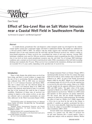
  • 17. and the Atlantic Ocean. The importance of well-field withdrawals was evaluated by running a simulation without groundwater withdrawals. The next simulation was used to evaluate the importance of droughts and annual variations in recharge. Dunn (2001) hypothesized that the 1971 to 1982 period of below average rainfall was partially responsible for the observed salt water intrusion event at the well field. To evaluate this hypothesis, a simulation was performed using a constant recharge rate calculated from the average annual rainfall total. Lastly, the utility of the artificial recharge system was evaluated by performing a simulation without artificial recharge. As shown in Figure 9, historical sea-level rise does not have a large effect on the position of the 1 g/L TDS contour in model layer 4, compared to the effect of pumping, but the effect is discernible. In 1955, for example, the 1 g/L contour for the simulation without sea-level rise is about 100 m seaward of the 1 g/L contour for the calibrated model. The largest effect from historical sea-level rise can be seen in 1995 near the southeastern part of the well field. In this area, the 1 g/L contour is as much as 1 km farther inland for the calibrated model than for the simulation without sea-level rise. This difference in the contour position is the result of the larger fresh water flux toward the coast for the simulation without sea-level rise. Thus, as sea level rises, the hydraulic gradient is reduced, the fresh groundwater flux decreases, and salt water intrusion occurs. This response is consistent with a head-controlled system. An analysis of simulated well-field TDS concentration (not shown) also indicates the effect of sea-level rise. The calibrated model shows an increase in TDS beginning in about 1971 and with TDS values exceeding the potable limit in 1984. Without a rise in sea level, the increase in TDS occurs within about a year of the calibrated model, but the well-field TDS concentration never exceeds the potable limit. Most importantly, well-field TDS concentrations are consistently about 0.2 g/L less from about 1980 to 2002 for the case without sea-level rise. Although this is a relatively small difference, it equates to a difference in chloride concentration of about 100 mg/L, which is important considering the drinking water standard is 250 mg/L. To further evaluate the head-controlled nature of the system in response to sea-level rise, the simulated water table from the calibrated model was compared to the simulated water table from the sensitivity simulation without sea-level rise. Over most of the model domain, the elevation of the water table compares to within about 0.02 m or less. Along a narrow band near the coast, however, the water table for the calibrated model is higher than the water table for the simulation without sea-level rise. Specifically, to the east of a line that connects structure G56 with G57 (the easternmost structures that separate the fresh water canals from the tidally influenced canals; Figure 1), there are no fresh water canals to act as a strong head control and the relatively high land surface elevations along the Atlantic Coastal Ridge allow the water table to rise without much restriction by evapotranspiration. The sensitivity analysis clearly indicates that wellfield withdrawals have the largest effect on the position Figure 9. Results from the qualitative sensitivity analysis showing simulated results for the base case and for simulations of constant recharge, no sea-level rise, no groundwater withdrawals, and no artificial recharge. Contours are of the 1 g/L TDS concentration in model layer 4. NGWA.org C. Langevin and M. Zygnerski GROUND WATER 17
  • 18. of the 1 g/L TDS contour (Figure 9). By eliminating pumping altogether, the 1 g/L TDS contour does not change appreciably and the slight changes shown in Figure 9 can be attributed to construction of the tidal finger canals, historical sea-level rise, and recharge variations. To further evaluate the effect of well-field withdrawals, a range of different withdrawal increases and decreases were simulated. By eliminating withdrawals altogether, there is no historical rise in TDS concentrations at the well field. Doubling withdrawals, however, show substantial increases in well-field TDS concentrations. Slight decreases in well-field withdrawal rates also have a large effect on well-field TDS concentrations. Had the actual well-field withdrawals been 25% to 50% less, model results suggest that salt water intrusion may not have been a concern. Sensitivity results indicate that rainfall variations and artificial recharge can affect salt water intrusion, but the effects are much less important than effects of well-field withdrawals. Results from the simulation with a constant recharge rate are similar to the base case calibrated model, suggesting that the 1971 to 1982 period of less-thanaverage rainfall was not a predominant cause of salt water intrusion near the well field (Figure 9). A likely explanation is that surface water was brought into the area during that time to maintain water levels of the primary canals (Hillsboro and Cypress Creek). These canals do not show a decrease in stage during that period (Figure 3), and would have provided recharge to the aquifer to compensate for the drought conditions. Model results suggest that artificial recharge at the Pompano Municipal Golf Course has a beneficial impact on salt water intrusion. In 1995, for example (Figure 9), elimination of artificial recharge in the sensitivity simulation results in the 1 g/L TDS contour being located as much as 1.5 km landward of the position in the base case calibrated model. Contour positions in 2005 also suggest that artificial recharge helps to prevent salt water from intruding near the well field. Sensitivity to Projected Rates of Sea-Level Rise A sensitivity analysis was performed with the Opt. 6 model using four different rates of projected sea-level rise and using the average annual hydrologic conditions (well-field withdrawals, canal stages, rainfall and artificial recharge, and evapotranspiration rates) from the last year of the calibration period (2005). Results from these 100year simulations cannot be used to predict future rates of salt water intrusion in response to sea-level rise, because the simulations do not include anthropogenic changes, alternative rainfall patterns from climate change, or well-field management strategies. The results can be used, however, to investigate the sensitivity of salt water movement to different rates of projected sea-level rise. For the first simulation, sea level was held constant at the average annual 2005 level. For the remaining three simulations, sea level linearly increased over the 100year simulation at rates of 24, 48, and 88 cm/century as estimated in the IPCC TAR (Church et al. 2001). Sea-level 18 C. Langevin and M. Zygnerski GROUND WATER Figure 10. Simulated well-field TDS concentration for the sensitivity analysis of projected rates of sea-level rise. The concentrations were calculated as a volumetric average for groundwater extracted from municipal wells at the Pompano Beach well field. rise was represented in the model by linearly increasing the stage of the Atlantic Ocean and tidal canals. Intraannual variations in sea level were not represented in these simulations. Figure 10 shows a plot of well-field TDS concentration relative to time for the four simulations. The well-field TDS concentration was calculated as a volumetric average using the withdrawal rates and simulated TDS concentrations at individual extraction wells. Use of average 2005 hydrologic conditions and a constant sea level result in TDS concentrations of the well-field exceeding drinking water standards after 70 years. This finding suggests that the 2005 withdrawal rates may not be sustainable with the 2005 hydrologic conditions. When sea-level rise is included in the simulations, drinking water standards are exceeded 10 to 21 years earlier (after 60 years for a rise of 24 cm/century; 55 years for a rise of 48 cm/century; and 49 years for a rise of 88 cm/century). Apparent rates of lateral salt water intrusion in model layer 4 were calculated from these sensitivity simulations using the 1 g/L TDS contour. They are referred to here as apparent because there is an upward component of groundwater flow near the well field, and thus, intrusion is not limited to horizontal movement. Apparent lateral intrusion rates are 15, 17, 18, and 21 m/year for the 0, 24, 48, and 88 cm/century sea-level rise rates, respectively. Webb and Howard (2010) reported lateral salt water intrusion rates (referred to as interface velocity in their work) for different ratios of hydraulic conductivity to recharge and for different rates of sea-level rise. Their largest reported intrusion rate was 4 m/year, which is about four to seven times less than the rates reported here, but similar considering the substantial differences between their simplified two-dimensional system and the Pompano Beach well-field area. Discussion The Pompano Beach well-field area and nearby coastal areas in southeastern Florida represent an endmember in the spectrum of impacts of sea-level rise on NGWA.org
  • 19. salt water intrusion. The following are a number of general observations about southeastern Florida that help explain why the shallow coastal aquifer system is particularly vulnerable to salt water intrusion caused by sea-level rise. 1. As shown by Werner and Simmons (2009), systems that are head controlled are more susceptible to salt water intrusion caused by sea-level rise than those that are flux controlled. For confined aquifers that are flux controlled, sea-level rise may not have any effect on salt water intrusion (Chang et al. 2011). The widespread canal system in southern Florida places an extensive head control on water levels in the shallow surficial aquifer. The head control is particularly strong in southeastern Florida due to the direct hydraulic connection between canals and the highly permeable Biscayne aquifer. Also, land surface is relatively flat with little relief, and the unsaturated zone is thin (typically less than a meter or two). Flooding from high water tables can be a problem in many neighborhoods. Evapotranspiration rates are also relatively high and can be similar to rainfall rates during the summer months. These combined conditions effectively eliminate the possibility for groundwater levels to rise as sea level rises. Consequently, the seaward hydraulic gradient and associated fresh groundwater flow toward the coast is expected to decrease. 2. Southeastern Florida has many tidally influenced canals that extend inland into the permeable coastal aquifer. In some cases, tidal canals extend inland as far as municipal well fields. These canals provide ocean access for a thriving boating community. Near the Pompano Beach well field, the tidal portion of the Cypress Creek Canal extends inland as far as the Pompano Beach well field. Tidal canals are also present between the well field and the Intracoastal Waterway. These tidal canals, which have elevated salinities, have stages at or near the stage of the Atlantic Ocean. A rising sea level makes it difficult to maintain a seaward hydraulic gradient that is strong enough to prevent salt water intrusion. 3. The highly permeable shallow aquifer system also contributes to the susceptibility of southeastern Florida to sea-level rise. The high hydraulic conductivities serve to reduce the seaward hydraulic gradient, cause rapid water level declines after aquifer recharge events, and allow salt water to intrude the aquifer at relatively fast rates. 4. Southeastern Florida is heavily populated with a large water demand for potable as well as for environmental purposes; nearly all of the potable water is derived from the shallow aquifer system, although there have been recent efforts to explore alternative water sources. Most groundwater is withdrawn near the coast at well fields located along the Atlantic Coastal Ridge. The Atlantic Coastal Ridge is the preferred location for well fields because additional treatment is often required for poorer quality groundwater withdrawn farther inland. Construction of the Palm Aire well field, located west NGWA.org of the Pompano Beach well field, was an effective mechanism for reducing groundwater withdrawals near the coast; shifting withdrawals inland raised the water table near the coast and reduced the threat of salt water intrusion. The modeling analysis described in this investigation can be used to quantify effects of sea-level rise for other areas. Therefore, it is important to summarize important and transferable lessons such as those related to dual-domain transport, grid resolution, computational issues, and modeling approach. Numerous challenges were encountered in the development and calibration of the county-scale (300 km2 ) dispersive salt water intrusion model. Representing solute transport with a dual-domain approach is consistent with geological knowledge of permeable flow zones in the Biscayne aquifer and seemed to provide a more accurate representation of salt water intrusion than the traditional advection-dispersion approach. Without the dual-domain approach, there was no way to calibrate the model (with a reasonable parameter set) so that it could simultaneously represent the salt water intrusion event and subsequent retreat of saline groundwater. Numerical dispersion and use of appropriate grid resolution and transport schemes were among the most difficult challenges. Sanford and Pope (2010) encountered the same problem for a large 2000 km2 salt water intrusion model of the Eastern Shore of Virginia and questioned whether concentrations at an individual well can be accurately simulated by a numerical model of that scale. They suggest that in some instances, 10-cm thick model layers may be required to accurately characterize the transition zone between fresh and saline groundwater. Owing to computational limitations, Sanford and Pope (2010) were not able to use the TVD scheme in MT3DMS/SEAWAT for their problem, which would have helped to reduce numerical dispersion as it did for the present application. For computation reasons, Sanford and Pope (2010) used the relatively fast, implicit finitedifference scheme for solute transport. This made the problem tractable with present computing technology. Additional numerical resolution would have been useful for the present study. The model was unable to represent some of the observed salinities in monitoring wells (e.g., G-2055); maximum concentrations tended to be underestimated, for example. There are many possible reasons why the model had difficulty in simulating the details of the salt water intrusion event (e.g., errors in the conceptual model or problems with the data); it would have been useful to eliminate numerical dispersion as a possibility. As shown by Langevin and Hughes (2009), calibration of a salt water intrusion model with a high level of numerical dispersion can have deleterious effects on the predictive capability of the model. If, for example, some of the hydraulic conductivity heterogeneity was introduced by the calibration process in order to compensate for the effects of numerical dispersion, then model predictions would be in error if the predictions were sensitive to that heterogeneity. As mentioned by Sanford C. Langevin and M. Zygnerski GROUND WATER 19
  • 20. and Pope (2010), the capability to add resolution where necessary is desirable in this situation. A finite element or finite volume model would have been one option. Another option for future studies would be to implement a local-grid refinement approach (Mehl and Hill 2002) in SEAWAT as a way to increase horizontal and vertical model resolution in areas where transport is important and predictions depend on accurate representation of large hydraulic gradients. For these types of larger-scale studies with potential difficulties in simulating dispersive solute transport, one might also consider an entirely different modeling approach based on an existing sharp interface formulation, which is available in the Salt Water Intrusion (SWI) Package for MODFLOW (Bakker 2003; Bakker and Schaars 2005). The sharp interface approach was designed for regional salt water intrusion modeling, and while it cannot simulate solute concentrations, it is by design, free of any type of dispersion including numerical dispersion. Calibration of the salt water intrusion model within a highly parameterized context was found to be useful for this study. The Pompano Beach well field consists of 16 groundwater withdrawal wells. Extraction rates for the wells are highly variable between wells and throughout time. The system also has many other spatially and temporally variable stresses (variations in fresh and tidal canal levels, recharge, artificial recharge, rainfall, evapotranspiration) that confound interpretation of hydrologic records. Karst aquifers, such as the Biscayne aquifer, are highly discontinuous and heterogeneous, both in their spatial and temporal functioning, and it is commonly difficult to separate the signal caused by a natural hydrologic event from one caused by an anthropogenic event. It was difficult to infer from the data subsurface areas that may be more or less permeable, and there were few reliable point measurements of hydraulic conductivity. With the highly parameterized calibration approach, features of the system were quantified by monitoring where and how parameters changed. In many instances, unrealistic parameter distributions were used to identify deficiencies in the numerical model, such as an erroneous prescribed canal level or an error in a monitoring well location. Although not considered in this assessment, a next step in this type of analysis is to quantify prediction uncertainty. Robust uncertainty measures can be calculated within the highly parameterized context provided one can assign measures of parameter uncertainty. Future efforts to quantify sea-level rise impacts would benefit from considering uncertainty quantification. Uncertainties in the predicted salt water intrusion patterns that result from sea-level rise were not quantified, but experience with the model suggests that there is a high level of uncertainty. As suggested by Konikow (2011) and experienced in this effort, solute transport models are particularly difficult to develop, and one should not expect the same level of reliability as one might expect for a groundwater flow model. Uncertainties caused by structural model errors can be reduced by evaluating differences in model simulations instead of focusing on 20 C. Langevin and M. Zygnerski GROUND WATER a specific numeric value produced from a single forward model run (Doherty and Welter 2010). For the sensitivity analysis of the projected sea-level rise, this means it is preferable to state that well-field concentrations exceed the potable limit 10 to 21 years sooner than for the case without sea-level rise. This study focused on evaluating the sea-level rise projections reported by the IPCC (Church et al. 2001). More recent projections by the IPCC (Meehl et al. 2007) seem to project sea level rising at a slower rate, but the revised estimates do not include some feedback mechanisms that are anticipated to occur, such as rapid ice sheet melting. Recent studies (Pfeffer et al. 2008) have shown that sea level may rise by 0.8 to 2.0 m by 2100. Heimlich et al. (2010) summarize some of the recent sea-level rise projections and their possible effects on southeastern Florida. These larger rates of sea-level rise were not tested with the model. It is reasonable to assume that increased rates of sea-level rise much larger than those considered here would have serious impacts on the fresh coastal groundwater supplies of southeastern Florida. For these larger rates of sea-level rise, it is unclear if adaptation measures and changes to the infrastructure could meet potable water demands while simultaneously providing flood protection. Conclusions Conditions near the Pompano Beach well field in northern Broward County, Florida, provide a unique opportunity to examine the effects of historical and projected sea-level rise on the fresh groundwater resources of a low-lying highly permeable coastal aquifer. Results of a numerical modeling analysis suggest that groundwater withdrawals were the dominant cause of a multi-decade salt water intrusion event, and that historical sea-level rise (about 25 cm for the simulation period) contributed to the extent of the intrusion by about 1 km. The historical rate of sea-level rise was similar to the lower-bound estimate (24 cm) of the IPCC (Church et al. 2001) projection for the next century. A sensitivity analysis of four projected rates of sea-level rise (24, 48, and 88 cm/century) comparatively illustrates the relative severity of the situation in south Florida. Even if sea level does not rise in the future, model simulations suggest that corrective actions would likely be required to protect the aquifer from salinization. Corrective actions would be required as much as 21 years sooner depending on the future rate of sea-level rise. The findings from this study are consistent with general observations about the vulnerability of southeastern Florida to salt water intrusion caused by sealevel rise. Southeastern Florida is particularly vulnerable because of (1) the overlying canal system, which acts as a strong head control, (2) the presence of tidal canals that extend inland, (3) the highly permeable shallow aquifer system, which includes the Biscayne aquifer, and (4) the large groundwater withdrawals from the coastal aquifer. NGWA.org
  • 21. Acknowledgments Special acknowledgments to Darrel Dunn and Katie Lelis of the Broward County Environmental Protection Department/Water Resources Division, Francis Henderson and Dave Markward of the Broward County Office of Environmental Services/Water Management Division, and Randy Brown, Maria Loucraft, and Alan Clark of Pompano Beach Utilities Department for providing extensive information and data on the study site. A special thanks to Winnie Said and Krista Guerrero-Reger of the South Florida Water Management District as well as Guy Bartolotta of Broward County Environmental Operation Division for providing model data sets and historical well-field pumping records, and to John Doherty for his continued support with the parameter estimation program (PEST). Technical assistance was also provided by Alyssa Dausman, Joann Dixon, and Roy Sonenshein. The authors are grateful to John Masterson, Jeremy White, and three anonymous reviewers for providing thoughtful comments that substantially improved the manuscript. References Andersen, P.F., J.W. Mercer, and H.O. White. 1988. Numerical modeling of salt-water intrusion at Hallandale, Florida. Ground Water 26, no. 5: 619–630. DOI: 10.1111/j.17456584.1988.tb00796.x Bakker, M. 2003. A Dupuit formulation for modeling seawater intrusion in regional aquifer systems. Water Resources Research 39, no. 5: 1131. Bakker, M., and F. Schaars. 2005. The Sea Water Intrusion (SWI) Package Manual, version 1.2. http://bakkerhydro.org/ swi/index.html (accessed January 2011). Bates, B.C., Z.W. Kundzewicz, S. Wu, and J.P. Palutikof, ed. 2008. Climate Change and Water. Technical Paper of the Intergovernmental Panel on Climate Change, 210. Geneva: IPCC Secretariat. Bredehoeft, J.D. 2003. From models to performance assessment: The conceptualization problem. Ground Water 41, no. 5: 571–577. Broward County Department of Planning and Environmental Protection (BCDPEP). 2001. Broward County, Florida Historical Water Quality Atlas: 1972-1997, Technical Report Series TR: 01-03, 418. Camp, Dresser, and McKee, Inc. 1980. Prospect well field impact analysis. Consultant report to the City of Fort Lauderdale, 96 p. Carrera, J., J.J. Hidalgo, L.J. Slooten, and E. Vazquez-Sune. 2010. Computational and conceptual issues in the calibration of seawater intrusion models. Hydrogeology Journal 18, no. 1: 131–145. Causaras, C.R. 1985. Geology of the surficial aquifer system. U.S. Geological Survey Water-Resources Investigations Report 84-4068. Broward County, Florida, 167, 2 sheets. Cazenave, A., and R.S. Nerem. 2004. Present-day sea level change: observations and causes. Reviews of Geophysics 42, no. 3, RG3001. DOI: 10.1029/2003RG000139 Chang, S.W., T.P. Clement, M.J. Simpson, and K.K. Lee. 2011. Does sea-level rise have an impact on saltwater intrusion? Advances in Water Resources 34, no. 10: 1283–1291. Church, J.A., J.M. Gregory, P. Huybrechts, M. Kuhn, K. Lambeck, M.T. Nhuan, D. Qin, and P.L. Woodworth. 2001. Changes in sea level. In Climate Change 2001: The Scientific Basis, ed. J.T. Houghton, Y. Ding, D.J. Griggs, M. Noguer, P.J. Van Der Linden, X. Dai, K. Maskell, and NGWA.org C.A. Johnson, 639–694. New York: Cambridge University Press. Cunningham, K.J., M.C. Sukop, H. Huang, P.F. Alvarez, H.A. Curran, R.A. Renken, and J.F. Dixon. 2009. Prominence of ichnologically influenced macroporosity in the karst Biscayne aquifer: stratiform “super-K” zones. Geological Society of America Bulletin 121, no. 1/2: 164–180. Cunningham, K.J., R.A. Renken, M.A. Wacker, M.R. Zygnerski, E. Robinson, A.M. Shapiro, and G.L. Wingard. 2006. Application of carbonate cyclostratigraphy and borehole geophysics to delineate porosity and preferential flow in the karst limestone of the Biscayne aquifer, SE Florida. In Perspectives on Karst Geomorphology, Hydrology, and Geochemistry—A Tribute Volume to Derek C. Ford and William B. White, 191–208, ed. R.S. Harmon, and C. Wicks. Geological Society of America Special Paper 404. Dausman, A.M., J. Doherty, C.D. Langevin, and J. Dixon. 2010. Hypothesis testing of buoyant plume migration using a highly parameterized variable-density groundwater model at a site in Florida, USA. Hydrogeology Journal 18, no. 1: 147–160. DOI: 10.1007/s10040-009-0511-6 Dausman, A.M., and C.D. Langevin. 2005. Movement of the saltwater interface in the surficial aquifer system in response to hydrologic stresses and water-management practices, Broward County, Florida. U.S. Geological Survey Scientific Investigations Report 2004-5256. Reston, Virginia: USGS. Doherty, J. 2009a. PEST, Model Independent Parameter Estimation. Addendum to user manual: 5th ed. Brisbane, Australia: Watermark Numerical Computing. http://www.sspa.com/ PEST/. Doherty, J. 2009b. PEST, Model Independent Parameter Estimation. User manual: 5th ed. Brisbane, Australia: Watermark Numerical Computing. http://www.sspa.com/PEST/. Doherty, J.E. 2009c. PEST Groundwater Data Utilities. Brisbane, Australia: Watermark Numerical Computing. Doherty, J. 2003. Groundwater model calibration using pilot points and regularisation. Ground Water 41, no. 2: 170–177. Doherty, J., and D. Welter. 2010. A short explanation of structural noise. Water Resources Research 46: W05525. DOI: 10.1029/2009WR008377 Dunn, D. 2001. Three-dimensional analysis of saltwater Intrusion: City of Pompano Beach Area, Broward County, Florida. Technical Report Series TR-01-06. Feseker, T. 2007. Numerical studies on saltwater intrusion in a coastal aquifer in northwestern Germany. Hydrogeology Journal 15, no. 2: 267–279. Fish, J.E. 1988. Hydrogeology, aquifer characteristics, and ground water flow of the surficial aquifer system, Broward County, Florida. U.S. Geological Survey Water-Resources Investigations Report 87–4034. Fujinawa, K., T. Iba, Y. Fujihara, and T. Watanabe. 2009. Modeling interaction of fluid and salt in an aquifer/lagoon system. Ground Water 47, no. 1: 35–48. DOI: 10.1111/ j.1745-6584.2008.00482.x Giambastiani, B.M.S., M. Antonellini, G.H.P. Oude Essink, and R.J. Stuurman. 2007. Saltwater intrusion in the unconfined coastal aquifer of Ravenna (Italy): A numerical model. Journal of Hydrology 340, no. 1–2: 91–104. Guha, H., and S. Panday. 2012. Impact of sea level rise on groundwater salinity in a coastal community of South Florida. Journal of the American Water Resources Association (JAWRA) 48, no. 3: 510–529. DOI: 10.1111/j.17521688.2011.00630.x Guo, W., and C.D. Langevin. 2002. User’s guide to SEAWAT: A computer program for the simulation of three-dimensional variable-density ground-water flow. U.S. Geological Survey Open-File Report 01-434. Harbaugh, A.W., E.R. Banta, M.C. Hill, and M.G. McDonald. 2000. MODFLOW–2000, the U.S. Geological Survey C. Langevin and M. Zygnerski GROUND WATER 21