Quline manual

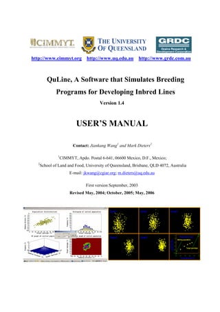
http://www.cimmyt.org http://www.uq.edu.au http://www.grdc.com.au

QuLine, A Software that Simulates Breeding
Programs for Developing Inbred Lines
Version 1.4

USER’S MANUAL

Contact: Jiankang Wang1 and Mark Dieters2

1
CIMMYT, Apdo. Postal 6-641, 06600 Mexico, D.F., Mexico;
2
School of Land and Food, University of Queensland, Brisbane, QLD 4072, Australia
E-mail: jkwang@cgiar.org; m.dieters@uq.edu.au

First version September, 2003
Revised May, 2004; October, 2005; May, 2006

Cycle 1 Cycle 2 Cycle 3

0
Cycle 4 Cycle 5 Population mean
10
Starting population
d is ta n c e (% )
H a m m in g

20
30
Target genotype
40
50
50 60 70 80 90 100
Target genotype (%)

QUCIM USER’S MANUAL, 6/1/2006

Contents
1. Introduction to QU-GENE and QuLine 2
2. Input file for the QU-GENE engine (QUG file) 4
2.1 General information about a GE system 4
2.2 Environment data 5
2.3 Trait data 5
2.4 Gene information 7
2.5 Population information 9
2.6 Diagnostic information 11
3. General information for a simulation experiment, and definition of breeding
strategies to be simulated by QuLine 17
3.1 General information for a simulation experiment 17
3.2 Definition of breeding strategies to be simulated 19
3.3 Definition of each breeding strategy 19
3.4 Definition of each generation 20
3.5 Definition of each selection round 21
4. Steps for running a simulation experiment using QuLine 32
4.1 Build the QUG file for the engine input 32
4.2 Run the QU-GENE engine to generate GES and POP files 32
4.3 Build the QMP file for the simulation experiment 33
4.4 Build the MIO files 33
4.5 Run QuLine 33
4.6 Outputs from running QuLine 33
5. Selected references 37
6. Abbreviations and acronyms 37
7. Acknowledgment 39

Page 1


QuLine: A Software that Simulates
Breeding Programs for Self-Pollinated Crops

USER’S MANUAL

Jiankang Wang, Maarten van Ginkel, Guoyou Ye, and Ian DeLacy

1. Introduction to QU-GENE and QuLine

The major objective of plant breeding programs is to develop new genotypes that are genetically
superior to those currently available for a specific target environment or a target population of
environments (TPE). To achieve this objective, plant breeders employ a range of selection methods.
Many field experiments have been conducted to compare the efficiencies from different breeding
methods. However, due to the time and effort needed to conduct field experiments, and their
associated errors, the concept of modelling and prediction have always been of interest to plant
breeders. Quantitative genetic theory generally provides much of the framework for the design and
analysis of selection methods used within breeding programs. However, various assumptions are made
in quantitative genetics in order to render theories mathematically or statistically tractable. Some of
these assumptions can easily be tested or satisfied by certain experimental designs; others can seldom,
if ever, be met, such as the assumptions of no linkage and no genotype by environment (GE)
interaction. Still others, such as the presence or absence of epistasis and pleiotropy, are difficult to test.
Computer simulation gives us the opportunity to lessen the impact of these assumptions, thereby
establishing more valid genetic models for use in plant breeding.

Simulation as a tool has been applied in many special plant breeding studies that use relatively
simple genetic models. However, a tool capable of simulating the performance of a breeding strategy
for a continuum of genetic models ranging from simple to complex, embedded within a large practical
breeding program including marker-assisted-selection, had not been available until recently. We
introduce just such a tool here: QU-GENE, a simulation platform for quantitative analysis of genetic
models that makes it possible to develop a general simulator for large breeding programs through its
two-stage architecture. The first stage involves QU-GENE as the engine, the role of which is to: (1)
define the GE system (i.e., all the genetic and environmental information for the simulation
Page 2

experiment), and (2) generate the initial population of individuals (base germplasm) and/or a reference
population to estimate genetic and/or environmental variances. The second stage involves the
application modules, whose role is to investigate, analyze, or manipulate the initial population of
individuals within the GE system defined by the engine. The application module usually represents the
operation of a breeding program. Within this two-stage architecture, the engine generates core
information for the GE system, and the details required for specific simulation experiments are defined
in the application modules. Thus simulation experiments are designed and implemented by developing
an application module that interacts with information generated by the engine. Thanks to this
architecture, QU-GENE has a high degree of flexibility. Numerous alternative simulation experiments
that combine breeding methods with a range of GE systems can be conducted to study the
performance of breeding methods under genetic models, including additive, dominance, and epistasis
genetic effects, GE interaction, pleiotropy, linkage, multiple alleles, and molecular markers.

Although QuLine is a QU-GENE strategic application module developed to simulate the wheat
breeding programs of the International Maize and Wheat Improvement Center (CIMMYT), the
breeding strategies defined in QuLine represent the operations of most breeding programs for self-
pollinated crops. Breeding methods that can be simulated by QuLine are mass selection, pedigree
selection, bulk-population selection, back cross breeding, top cross (or three-way cross) breeding,
doubled haploid breeding, marker-assisted selection, and any combination or modification of these
methods. Simulation experiments can therefore be designed to compare the breeding efficiencies of
different selection strategies, or various modifications within a selection strategy. To run a simulation
experiment in QuLine, we need:

(1) Two software programs: the QU-GENE engine (called QUGENE) and QuLine, the
application module;

(2) Two input files: the QUG file for QUGENE and the QMP file for QuLine. There are two
types of output files after running the engine: a GES file to define the GE system and a POP
file to define a initial population for a breeding program. QuLine will use a combination
consisting of a GES, a POP, and a QMP file as its input.

2. Input file for the QU-GENE engine (QUG file)

The QUG file contains all the information required to define a genotype and environment (GE) system
and the initial population to which the breeding method will be applied. The GE system underlies the

Page 3

genetic and environmental model framework for simulation experiments. In general, information
about a GE system consists of general information about the GE system, the target population of
environments (TPE) for the breeding program, traits to be selected during the breeding procedure,
random environmental deviations for these traits, genes for traits, their locations on chromosomes, and
their effects on traits in different environment types. Information about the population consists of the
number of parents and their genotypes. The sample QUG file shown in Table 1 can be used as a
template for any GE system.

2.1 General information about a GE system

The first part of a QUG file is general information about the GE system (Table 1).

(1) Number of models. This parameter is specifically designed for a GE system with random gene
effects. For a GE system with all gene effects (additive, dominance, epistasis, and pleiotropy)
fixed, this parameter should be set at 1. The random effects model in a GE system will most
likely mimic the real genetic effects of a large number of genes, such as the genes for yield.
With this model some genes will have relatively larger effects and others, smaller effects. The
large number of GE systems, different yield gene effects in each GE system, and replications
feasible within the simulation allow many potential realities to be compared. If one breeding
methodology is superior to another for all, or most, permutations, the breeder can be confident
that a superior breeding methodology has been identified that is also robust to the complexities
and perturbations that may emerge, regardless of the GE system.

(2) Random seed of random gene effects. This random seed will ensure that the same gene effects
will be assigned whenever the GE system is used, so that all random gene effects are
repeatable.

(3) Number of genes. Number of genes (including markers) in the GE system.

(4) Number of environments. Number of environment types in TPE for the GE system.

(5) Number of traits. All traits (excluding marker scores) used in selection should be counted.

(6) Specify names. There are 7 indicators (a one-dimension array with size 7, each element is equal
to either 0 or 1) reporting whether the names for environment types, traits, genes (loci), alleles,
epistasis network, genotype to phenotype mapping, and populations, respectively, will be
specified in the QUG file. 0 = no name specification; 1 = name specification (valid name
required).

Page 4

2.2 Environment data

The TPE for a breeding program consists of a set of distinct, relatively homogenous environment types,
each with a frequency of occurrence. Each environment type has its own gene action and interaction,
providing the framework for defining GE interactions. There are three parameters for defining each
environment type (Table 1):

(1) Row 1: Environment number. To distinguish each environment type.

(2) Row 2: Name of the environment type (if defined). If the indicator for environment type names
is 1, a valid name must be specified for each environment type. If the indicator for
environment type names is 0, the place is left blank.

(3) Row 3: Frequency of occurrence in the TPE. The sum of all frequencies should be equal to 1.0.

Environment data are stored in the Env(:) array data type in the GE system definition (Fig. 2).
The number of environment types can be calculated from the array size.

2.3 Trait data

For the purpose of simulation, the genotypic value of an individual can be calculated from the
definition of gene actions in the GE system and from its genotypic combination. However, breeders
select based on the phenotypic value in the field. Therefore, the phenotypic value of a genotype in a
specific environment needs to be defined from its genotypic value and associated environmental errors.
For example, if there are n plots (or replications) for a family and the plot size is m, there will be
n × m individual plants (or genotypes) for this family. The genotypic value g ij ( i = 1, L, n ; j = 1, L m )

can be defined from the GE system, and the phenotypic value pij can then be calculated using the

formula pij = g ij + eib + eij , where eib is the between-plot error for plot i, and eij is the within-plot
w w

error for genotype j in plot i, and both eij and eib are assumed to be normally distributed. The variance
w

( σ e2 ) of ewij is either user specified or calculated from the definition of heritability in the broad sense

σg2

h = 2
2
, where the genetic variance ( σ g ) is calculated from the genotypic values of individuals
2

σ g + σ e2
b

in the specified reference population in the QUG file. In a simulation experiment, the variance of eib

can be set to be a proportion of σ e2 (i.e. Var (ebi ) = rσ e2 ), where the value of r is based on field data or

experience. In some environments, r can be 1.5 or 2.0; in others, 1.0 or even lower. This proportion

Page 5

will affect the efficiency of among-plot (family) selection. Lower r means higher among-plot selection
efficiency, and higher r means lower selection efficiency. Once the genotypic value of a genotype has
been defined, a random effect for between-plot error from the distribution N (0, rσ e2 ) and a random

effect for within-plot error from the distribution N (0, σ e2 ) will be added to the genotypic value g ij to

give the phenotypic value pij . The family mean can then be calculated from pij . QuLine then

simulates within-family selection using phenotypic values and among-family selection using family
means. For multiple traits, QuLine uses the independent selection process for both types of selection.

The trait data will let QuLine define the phenotypic value from the genotypic value. Therefore,
the major trait information required by the QU-GENE engine is the environmental effects on traits
(within-plot variance and among-plot variance) in each environment type. Either the variance or
individual plant-level heritability in the broad sense needs to be specified. For heritability, the QU-
GENE engine will convert the specified heritability into an estimate of environmental variance based
on the provided reference population. This environmental variance is used throughout the simulation.
The population structure differs from generation to generation; hence, population heritability also
varies with changes in the genetic variation within the population.

There are four parameters for defining the trait data (Table 1).

(1) Row 1: Trait number. To distinguish each trait.

(2) Row 2: Name of the trait (if defined). If the indicator for trait names is 1, a valid name must be
specified for each trait or the place is left blank.

(3) Row 3: Error specification type. One-dimension array with size 3 for three kinds of error:
within-plot, among-plot, and mixture-plot (not complemented yet). Two alternative values for
each element:

• 1 = for the individual plant level heritability in the broad sense for within-plot; for the
proportion to within-plot error variance for among-plot.

• 2 = for error variance itself.

(4) Row 4+: Within-plot, among-plot and mixture-plot errors for all the defined environment types.
If error specification type is equal to 1, the value indicates heritability for within-plot, and
proportion of within-plot error variance for among-plot. If error specification type is equal to 2,
the specified value is for random environmental effect variance on the trait.

Page 6

2.4 Gene information

Gene information is the most fundamental and complicated part of defining a GE system. It is used to
generate progeny genotypes from any crossing or propagation type, and to define the genotypic value
of any genotype for each trait. It consists of the location of genes on wheat chromosomes, the number
of alleles for each gene locus, the number of traits affected by each gene, the genotypic effects in each
defined environment type, etc. Linkage, multiple alleles, pleiotropy, epistasis, and GE interaction are
all defined in this part. The following parameters define each gene (including markers) (Table 1).

(1) Row 1: Gene (locus) number. To distinguish each gene.

(2) Row 2: Name of the gene (if defined). If the indicator for gene name is 1, a valid name must be
specified, or the place is left blank.

(3) Row 3: Chromosome, recombination frequency, number of alleles, and number of traits the
gene affects. All the genes, including markers, in the GE system are supposed to be arranged in
order on the chromosomes. Recombination frequency of a gene is the crossover rate between
the gene and the gene located just before it (two flanking genes). If a gene is located at the
beginning of a chromosome, its recombination frequency should be set at 0.5.

(4) Row 4: Name of each allele (if defined). If the indicator for allele names is 1, a valid name
must be specified for each allele, or the place left blank.

(5) Row 5+: QTL information

• Column 5: Trait(s) the gene affects.

• Column 6: Environment type.

• Column 7: Genotype to phenotype mapping (gene effect type).

o 1 = additive and dominant gene without epistasis.

o 2 = epistatic gene.

o 3 = QU-GENE plug-in gene (not complemented yet).

• Column 8: How gene effects are stored.

o For additive genes (Option 1 for Column 7):

Page 7

–1 = midpoint (m); additive (a) and dominance (d) will be specified later.
This option is only available for genes with two alleles. For a gene with
multiple alleles, option 0 should be used.

0 = genotypic values in the order of AA, Aa, and aa, where A-a are the
two alternative alleles on the gene locus. In case of three alleles (A1-A2-
A3), the values are arranged in the order of A1A1, A1A2, A1A3, A2A2,
A2A3, and A3A3. The order is similar for more than three alleles at a
gene locus.

1 = random gene effects with no dominance. Genotypes AA and aa have
random values AA and aa ranged from 0.0 to 1.0, but the value (Aa) of
genotype Aa is at the mid point between AA and aa, i.e.
Aa = 1 ( AA + aa ) .
2

2 = random gene effects with no over-dominance. Genotypes AA, Aa
and aa have random values ranged from 0.0 to 1.0, but Aa is between AA
and aa.

3 = random gene effects with partial/over-dominance. Genotypes AA,
Aa and aa have independent random values ranged from 0.0 to 1.0,
which will result in either partial dominance or over-dominance,
depending on chance.

o For epistatic genes (Option 2 for Column 7):

Which epistatic network the gene is in.

o For QU-GENE plugin genes (Option 3 for Column 7):

Which plugin the gene is in (not complemented yet).

(6) Row 5+: Marker information

• Column 5: Trait number has to be set at 0. Trait number 0 is reserved to identify which
gene locus is a marker.

• Column 7: Marker definition type.

o 0 = explicit values for marker types MM, Mm, and mm.

Page 8

o 1 = marker is dominant.

o 2 = marker is co-dominant.

• Column 8: Which gene has the marker (if required).

• Column 9: Values for each allelic combination (if required).

2.5 Population information

For a population, the most important information is the allelic combination for each individual in the
population (Fig. 3). There are basically two ways to define a population in the QUG file. One is to
define the gene frequencies in the population; then the QU-GENE engine will generate a specified
number of genotypes based on gene frequencies. The other is to specify the genotype of each
individual in the population. In the QUG file, the number of populations to be created and the
population used to estimate environmental errors (i.e., the reference population) should be given first,
followed by the definition for each population. For each population the following information should
be provided (Table 1):

(1) Row 1: Population number. To distinguish each population.

(2) Row 2: Output file name for the population. The extension is automatically set as POP.

(3) Row 3: Population name (if defined). If the indicator for population names is 1, a valid name
must be specified for each population, or the place left blank.

(4) Row 4: Population size. Number of individuals in the population.

(5) Row 5: Population creation type.

• 1 = create population (alleles) (see pop1 in Table 1). The engine will assign an allelic
combination to each individual in the population based on the specified gene
frequencies.

• 2 = define allele frequencies only (a random seed number is required after this creation
type). Only the gene frequencies are recorded for the population. The allelic
combination for each individual is determined at the application stage (see pop2 in
Table 1).

• 3 = specify alleles (see pop3 in Table 1). For this option all allelic combinations in the
population need to be known.

Page 9

For population creation types 1 and 2:

(6) Row 6+: Information for each gene in the population.

• Column 1: Gene number. If the gene number is equal to 0, all the genes have the same
specifications (see pop4 in Table 1).

• Column 2: Allele order type.

o 1 = normal order.

o 2 = allele of interest first.

o 3 = allele of interest under background first.

• Column 3: Gene sampling type.

o 1 = population has the exact gene frequencies.

o 2 = population has the sampled gene frequencies.

• Column 4: Zygosity type.

o 1 = both hetero-zygosity and homo-zygosity are included in the population.
Genotypes AA, Aa and aa have the frequencies p2, 2pq and q2, where p is the
allele frequency of A and q is the allele frequency of a.

o 2 = homozygous only. Genotypes AA and aa have the frequencies p and q,
where p is the allele frequency of A and q is the allele frequency of a.

• Column 5: Linkage type in heterozygosity. This parameter tells how genes in double
hetero-zygosity in the population, such as AaBb, are arranged on the chromosome.

o 1 = coupling (for AB/ab).

o 2 = repulsive (for Ab/aB).

• Column 6: Genotype combination manipulation type.

o 0 = no manipulation.

o 1+ = genotype combination is the same as gene defined.

• Column 7+: Allele frequency (for two alleles) or allele frequencies (for multiple alleles).
If the number of alleles in the locus is n, n-1 values should be specified.

Page 10

For population creation type 3, all the genotypes in the population have to be defined. The
definition of each genotype is in the following order:

• Genotype number.

• Genotype name.

• Allele combination on the first set of homologous chromosomes.

• Allele combination on the second set of homologous chromosomes.

2.6 Diagnostic information

There are two diagnostic parameters at the end of a QUG file; one is for the GE system and the other
is for the population. The output information will be recorded in the file whose prefix name is the
same as the GE system and the extension is DGN. There are three options for each of the two
parameters.

• 0 = no information output

• 1 = summary information output

• 2 = detailed information output

Table 1. Sample input file for the QU-GENE engine
*** Version 2.2.01 - 1st June 2002 ***
! ************************************************************************
! * QUGENE engine input file
! ************************************************************************

! *** General information on the G-E system ***
! Engine G-E output filename prefix (*.ges)
test

2 ! Number of models
0 ! Random seed of random gene effects
22 ! Number of genes (includes markers and qtls)
3 ! Number of environment types
10 ! Number of traits (not including markers)
1 1 0 0 0 0 0 ! Specify names (ETs, Trts, Genes, Alls, EPN, GPM, pop)

! ************************************************************************
! *** Environment Type Information ***
! Row 1: Number
! Row 2: Name (if defined)
! Row 3: Frequency of occurrence in TPE
! ************************************************************************

1
ET1
0.5000

2

Page 11

ET2
0.3000

3
ET3
0.2000

! ************************************************************************
! *** Trait Information ***
! Row 1: Number
! Row 3: Error Specification Type (for within,among,mixture)
! 1=heritability (spb); 2=error
! Row 4+: Within, Among, Mixture error [each ET]
! ************************************************************************

1
Yield
1 1 2
0.0500 2.0000 0.0000
0.1000 2.0000 0.0000
0.1200 2.0000 0.0000

2
Lodging
2 2 2
1.5000 0.2000 0.0000
1.7000 0.3000 0.0000
1.9000 0.2000 0.0000

3
SR
1 2 2
0.5000 0.5000 0.0000
0.5000 0.5000 0.0000
0.5000 0.0000 0.0000

4
LR
1 2 2
0.0500 0.5000 0.0000
0.0500 0.5000 0.0000
0.0500 0.5000 0.0000

5
SR
1 2 2
0.5000 1.0000 0.0000
0.5000 0.5000 0.0000
0.5000 0.5000 0.0000

6
Height
1 2 2
0.5000 0.0000 0.0000
0.5000 0.0000 0.0000
0.5000 0.0000 0.0000

7
Tillering
1 2 2
0.5000 0.0000 0.0000
0.5000 0.0000 0.0000
0.5000 0.0000 0.0000

8
Heading
1 2 2
0.5000 0.0000 0.0000
0.5000 0.0000 0.0000
0.5000 0.0000 0.0000

9

Page 12

GRN/SPK
1 2 2
0.5000 0.0000 0.0000
0.5000 0.0000 0.0000
0.5000 0.0000 0.0000

10
TKW
1 2 2
0.5000 0.0000 0.0000
0.5000 0.0000 0.0000
0.5000 0.0000 0.0000

! ************************************************************************
! *** Gene Information ***
! Row 1: Number (0=same for all genes)
! Row 2: Gene name (if defined)
! Row 3: Chromosome; RF; No. of alleles; No of traits
! Row 4+: Name for each allele (if defined)
! Row 5+: (QTL)
! Column 5: Which trait
! Column 6: Environment type
! Column 7: G-P mapping type
! 1=additive gene
! 2=epistatic gene
! 3=QU-GENE plugin gene
! Column 8: Identifies how effects are stored
! For Additive genes:
! -1 = midpoint,additive, dominance
! 0 = explicit values (AA, Aa, aa)
! 1 = random effects with no dominance
! 2 = random effects with no over-dominance
! 3 = random effects with partial/over-dominance
! For Epistatic genes:
! Epistatic Network
! For QU-GENE plugin genes:
! Plugin mapping number
! Column 9+: Values for each allelic combination (if required)
! Row 5+: (Markers)
! Column 5: Trait 0
! Column 7: Marker definition type
! 0 = explicit values (AA, Aa, aa)
! 1 = marker is dominant
! 2 = marker is co-dominant
! Column 8: Which gene has marker (if required)
! Column 9+: Values for each allelic combination (if required)
! ************************************************************************
! Columns
! 1 2 3 4 5 6 7 8 9+
! ************************************************************************

1
1 0.500000 2 1
1 1 1 0 0.70000 0.50000 0.30000
2 1 0 1.00000 0.60000 0.00000
3 1 -1 0.50000 0.50000 0.00000
2
1 0.050000 2 1
1 1 1 -1 0.50000 0.50000 0.00000
2 1 -1 0.50000 -0.50000 0.00000
3 1 -1 0.50000 -0.50000 0.00000
3
1 0.050000 2 1
2 1 1 0 0.30000 0.50000 0.70000
2 1 -1 0.50000 -0.50000 0.00000
3 1 1
4
1 0.050000 3 1
2 1 1 0 1.00000 0.50000 0.70000 0.60000 0.50000 0.80000
2 1 0 0.50000 0.60000 0.90000 1.10000 1.50000 1.20000
3 1 0 1.60000 0.10000 0.30000 0.70000 0.80000 0.80000
5
1 0.050000 2 2

Page 13

2 1 1 0 0.90000 0.80000 0.70000
2 1 0 0.70000 0.20000 0.10000
3 1 0 0.70000 0.80000 0.60000
3 1 1 0 2.40000 1.80000 1.20000
2 1 0 3.20000 2.30000 1.70000
3 1 0 1.70000 2.50000 2.60000
6
2 0.500000 2 0
0 0 2.00000 2.00000 0.00000
7
2 0.050000 2 0
0 1 8
8
2 0.025000 2 1
0 0 2.00000 1.00000 0.00000
3 1 1 0 2.40000 1.80000 1.20000
2 1 0 3.20000 2.30000 1.70000
3 1 0 1.70000 2.50000 2.60000
9
2 0.035000 2 1
4 1 2 1
2 2 1
3 1 0 1.30000 0.80000 0.60000
10
2 0.050000 2 1
4 1 2 1
2 2 1
3 2 2
11
3 0.500000 2 1
4 1 1 0 1.30000 0.80000 0.60000
2 1 0 1.30000 0.80000 0.60000
3 2 2
12
3 0.500000 3 2
4 1 1 0 0.80000 0.40000 0.50000 1.30000 0.80000 0.60000
2 1 0 0.50000 1.30000 0.80000 1.00000 0.80000 0.60000
3 2 2
5 1 1 0 4.00000 3.20000 1.20000 3.00000 2.00000 3.20000
2 1 0 4.00000 3.20000 1.20000 3.00000 2.00000 3.20000
3 1 0 4.00000 3.20000 1.20000 3.00000 2.00000 3.20000
13
4 0.500000 2 1
6 1 1 1
2 1 2
3 1 2
14
5 0.500000 2 1
6 1 1 1
2 1 2
3 1 2
15
6 0.500000 2 1
7 1 1 1
2 1 2
3 1 2
16
7 0.500000 2 1
7 1 1 1
2 1 2
3 1 2
17
8 0.500000 2 1
8 1 1 1
2 1 2
3 1 2
18
9 0.500000 2 1
8 1 1 1
2 1 2
3 1 2
19
10 0.500000 2 1
9 1 1 1

Page 14

2 1 2
3 1 2
20
11 0.500000 2 1
9 1 1 1
2 1 2
3 1 2
21
12 0.500000 2 1
10 1 1 1
2 1 2
3 1 2
22
13 0.500000 2 1
10 1 1 1
2 1 2
3 1 2

! ************************************************************************
! *** Epistatic Network Information ***
! Row 1: Number
! Row 3: Fitness Type
! 0=values specified; 1=random
! Row 4+: Specified values (if required)
! ************************************************************************

1
0
1.0 0.400 0.500 0.200 0.400 0.600 0.500 0.600 0.800

2
1

! ************************************************************************
! *** Population Information (*.pop) ***
! Row 1: Number of populations to create
! Row 2: Which population to use for error estimates
!
! For each population:
! Row 1: Number
! Row 2: Output filename prefix (*.pop)
! Row 4: Population size
! Row 5: Population Creation Type
! 1=create population (alleles)
! 2=define allele frequencies only
! (Row 6: Random Seed)
! 3=specify alleles
! Row 6+:
! Column 1: Gene (0=same for all genes)
! Column 2: Allele order type
! 1 = normal order; 2=allele of interest first
! 3 =allele of interest (avg background) first
! Column 3: Gene Sampling Type
! 1 = population has exact gene frequencies
! 2 = population has sampled gene frequencies
! Column 4: Zygosity type
! 1=both hetero & homo produced; 2=homo only
! Column 5: Linkage Disequilibrium Type of Hetero
! 1=coupling; 2=replusion
! Column 6: Manipulate genotype combinations type
! 0=no manipulation; 1+=genotype combinations
! same as gene defined
! Column 7+: Allele frequenc(ies) (No. of alleles-1)
! ************************************************************************

4 ! Number of populations to create
1 ! Which population to use for error estimates

Page 15

1
pop1
20
1
1 2 2 1 1 0 0.2500
2 2 2 1 1 0 0.2500
3 2 2 1 2 0 0.2500
4 2 2 1 1 0 0.2500 0.2500
5 2 2 1 1 0 0.2500
6 2 2 1 1 8 0.2500
7 2 2 1 1 8 0.2500
8 2 2 1 1 0 0.2500
9 2 2 1 1 0 0.2500
10 2 2 1 1 0 0.2500
11 2 2 1 1 0 0.2500
12 2 2 1 1 0 0.2500 0.2500
13 2 2 1 1 0 0.2500
14 2 2 1 1 0 0.2500
15 2 2 1 1 0 0.2500
16 2 2 1 1 0 0.2500
17 2 2 1 1 0 0.2500
18 2 2 1 1 0 0.2500
19 2 2 1 1 0 0.2500
20 2 2 1 1 0 0.2500
21 2 2 1 1 0 0.2500
22 2 2 1 1 0 0.2500

2
pop2
50
2
43223
1 2 2 2 1 0 0.5000
2 2 2 2 1 0 0.5000
3 2 2 2 1 0 0.5000
4 2 2 2 1 0 0.5000 0.2500
5 2 2 2 1 0 0.5000
6 2 2 2 1 8 0.5000
7 2 2 2 1 8 0.5000
8 2 2 2 1 0 0.5000
9 2 2 2 1 0 0.5000
10 2 2 2 1 0 0.5000
11 2 2 2 1 0 0.5000
12 2 2 2 1 0 0.5000 0.2500
13 2 2 1 1 0 0.5000
14 2 2 1 1 0 0.5000
15 2 2 1 1 0 0.5000
16 2 2 1 1 0 0.5000
17 2 2 1 1 0 0.5000
18 2 2 1 1 0 0.5000
19 2 2 1 1 0 0.5000
20 2 2 1 1 0 0.5000
21 2 2 1 1 0 0.5000
22 2 2 1 1 0 0.5000

3
pop3
5
3

1
P1
11231 22111 22 2 1 2 2 1 1 1 2 2 2
11231 22111 22 2 1 2 2 1 1 1 2 2 2

2
P2
21212 21121 13 1 1 2 1 1 2 1 2 1 2
21212 21121 13 1 1 2 1 1 2 1 2 1 2

3
P3
12211 21112 11 2 2 1 1 2 2 2 2 2 2

Page 16

12211 21112 11 2 2 1 1 2 2 2 2 2 2

4
P4
12111 11111 22 2 2 2 1 1 2 1 1 2 2
12111 11111 22 2 2 2 1 1 2 1 1 2 2

5
P5
21221 22111 22 2 1 2 2 1 2 2 2 1 1
21221 22111 22 2 1 2 2 1 2 2 2 1 1

4
pop4
60
1
0 2 2 1 1 0 0.2500

! ************************************************************************
! *** Diagnostic Information (*.dgn) ***
! Column 1: G-E System
! 0=no information is output
! 1=summary information output
! 2=detailed information output
! Column 2: Population
! 0=no information output
! 1=summary information output
! 2=detailed information output
2 1

3. General information for a simulation experiment and definition of breeding strategies to be
simulated by QuLine

The data structure for defining breeding strategies in QuLine is shown in Fig. 1. In this section
CIMMYT’s wheat breeding program will be used as an example where appropriate (Fig. 2; Fig. 3;
Table 2). Other breeding methods for self-pollinated crops, such as mass selection, family selection in
S1, family selection in S2, traditional pedigree system, modified pedigree, bulk population breeding,
doubled haploid in F2, doubled haploid in F3, are given in Table 3.

3.1 General information for a simulation experiment

Ten parameters are included in this information.

(1) Number of strategies. Number of breeding strategies included.

(2) Number of runs. This is the number of replications for each model in the GE system. The
number of models is 1 if there is no random gene effect in the GE system.

(3) Number of cycles. See section 3.2 for an explanation of a breeding cycle.

(4) Number of crosses. The same crosses will be made for all simulated strategies in the first
breeding cycle, so the strategies can be properly compared.

Page 17

(5) Indicator for crossing block update.

• 0 = only the final selected lines are used as the parents for next breeding cycle. The
parents in the current crossing block will not be considered for crossing in the
following cycles.

• 1 = for the next cycle, some parents come from the current crossing block, and some
from the final selected lines.

(6) Indicator for GE system output.

• 0 = No output of GE system information.

• 1 = Output the GE system information model by model.

(7) Indicator for population output.

• 0 = No output.

• 1 = Output information about the population before selection and the population after
each cycle of selection, including genotypes, genotypic values, gene frequencies,
Hamming distance, genetic variances, etc.

(8) Indicator for selection history output.

• 0 = No output.

• 1 = Output the selection history of each line in the final selection population after each
breeding cycle.

(9) Indicator for Rogers distance output.

• 0 = No output.

• 1 = Output the Rogers distance for each cross, the lines from each cross after each
round of selection, and lines above the mid-parent and line above the better parent at
the end of a breeding cycle.

(10) Indicator for correlation output.

• 0 = No output.

• 1 = Output the correlation coefficients among traits in each environment type and
among environment types for each trait in the initial and selected populations.

Page 18

(11) Indicator for genetic variance components output.

• 0 = No output.

• 1 = Output the genetic variance components in each environment type and among
environment types for each trait in the initial and selected populations.

(12) Parents for all crosses.

• If ‘random’ is specified, no information for parents for all crosses is required. The
parents for each cross will be randomly specified in QuLine.

• Otherwise, the input will be an existing external file containing the parents for each
cross. Six parents are needed for each cross, i.e., the two parents for the single crossing,
the backcrossing parent, topcrossing parent, and the last two parents for double crossing.

The four nested loops in QuLine should be introduced here to clarify the difference between the
number of models in the GE system and the number of runs in the simulation experiment. The first
layer loop is the loop for all models. Within this loop, the parents for all crosses in the first breeding
cycle are determined. The next loops are all strategies, for all runs, and all cycles. So the difference
among runs reflects the difference among breeding strategies, as all the strategies start from the same
point, i.e., the same crossing block (initial population) and the same crosses.

3.2 Definition of breeding strategies to be simulated

A breeding strategy (Fig. 3; Table 2; Table 3) is defined in QuLine as all the crossing, seed
propagation and selection activities, and experimental designs in an entire breeding cycle. A breeding
cycle begins with crossing and ends at the generation when the selected advanced lines are returned to
the crossing block as new parents. Most breeding programs of self-pollinated crops can be described
approximately as shown in Fig. 3. This figure demonstrates the germplasm flow from making single
crosses in CIMMYT’s bread wheat breeding program. The selection method described in Fig. 3 is
called selected bulk at CIMMYT and will be used as an example to demonstrate how a breeding
strategy can be defined in QuLine. It should be noted that variations of this selection approach are
commonly used in breeding programs for self-pollinated crops.

Several breeding strategies can be defined simultaneously in one input file (QMP file) (see data
type Strategies in Fig. 1). The QuLine module then makes the same crosses for all the defined
strategies in the first breeding cycle. Hence, all strategies start from the same point (the same crossing

Page 19

block, the same crosses and the same GE system). All the strategies have to be defined. For each
breeding strategy, the following information in sections 3.2 to 3.4 is required.

3.3 Definition of each breeding strategy

Each breeding strategy needs to be defined separately. The definition of a strategy consists of the
following three parts:

(1) Strategy title; name of the breeding/selection method.

(2) Number of generations in the strategy.

(3) Definition of each generation.

In the breeding program shown in Fig. 3, the best advanced lines developed from the F10
generation will be returned to the crossing block to be used for new crosses; i.e., a new breeding cycle
starts after F10. Therefore the number of generations in one breeding cycle is 10 for the selected bulk
breeding strategy. Each of the 10 generations, along with the crossing block (viewed as F0), needs to
be defined (Fig. 1).

There are three key Mexican locations involved in this breeding program: Ciudad Obregon (27°
N, 39 m above sea level [masl]), Toluca (19° N, 2640 masl), and El Batan (19°N, 2300 masl) (Fig. 2).
Ciudad Obregon is an arid, irrigated location, and growing season conditions are similar to many other
irrigated environments around the world. Yield trials for materials targeted to low rainfall and irrigated
areas are conducted in Ciudad Obregon, where high yields are obtained (8-11 t/ha) and the main
diseases are leaf rust (Puccinia recondita) and stem rust (Puccinia graminis). Precipitation in Toluca
is high (about 800 mm during the summer crop cycle), providing favorable conditions for foliar
diseases, in particular stripe rust (Puccinia striiformis) and foliar blights, such as Septoria tritici.
Precipitation at CIMMYT Headquarters, El Batan, is more erratic, with an annual average of 500-600
mm; irrigation facilities are available when needed. El Batan is used mainly for leaf rust screening and
small-scale seed increases. Two crop cycles can be grown each year: November – April in Ciudad
Obregon, and May – October in Toluca and/or El Batan. These environment types and their
frequencies of occurrence in a specific breeding program should be defined in a GES file.

3.4 Definition of each generation

The parameters to define a generation consist of the number of selection rounds in the generation, the
indicator for seed source (explained below), and planting and selection details for each selection round
(Tables 2 and 3; Fig. 4). Most generations in Fig. 5 have just one selection round (e.g., F1 to F6),

Page 20

while some generations have more than one (e.g., F7, F8 and F9). Take the F7 as an example: once an
advanced line is selected from among F7 head-rows, the F8 seed lot is split three ways. A reserve is
kept for sowing yield trials at Ciudad Obregon in the following winter season [F8(YT)]; of the other
two sets, one is sown at Toluca [F8(T)] and another at El Batan [F8(B)] during the summer to evaluate
response to the respective disease spectra in the field. The entries composing the yield trial in the F8
generation [F8(YT)] in Ciudad Obregon are only those entries that have been proven resistant to the
diseases at the two summer locations [F8(T) and F8(B)]. The F7 generation is therefore subjected to
four rounds of selection: one among F7 lines, two based on disease evaluation in the field on progeny
(F8) in both Toluca and El Batan, and one based on F8 yield performance in Ciudad Obregon. Since
seed of the two F8 field disease evaluations and the F8 yield trial is derived from selected F7 lines (Fig.
5), the indicator of the seed source is 0 for F7 (Table 2). In other selection procedures the seed for
selection round i (i>1) may come from plants selected from round i-1. In that case the indicator for
seed source is denoted as 1. For those generations subjected to just one round of selection, no indicator
for the seed source is required (Table 2).

The simulation module was developed such that the key components of the field breeding
process were retained. This is important firstly for the integrity of the simulation, but also to allow the
breeder to retain confidence in the value of the simulation process. In practice, the F8 field disease
evaluation tests in Toluca (F8(T)) and El Batan (F8(B)) are grown in the same year as the F8 yield
trial (F8(YT)); the F8 small plot evaluation (F8(SP)) in Ciudad Obregon is grown just six months later
(Fig. 5). Using the starting conditions and selection intensities outlined in Table 3, there would be
14,760 F7 lines in the field derived from pedigree selection in F6. Following F7 selection, 3,868 are
promoted to F8 disease evaluation in the field in Toluca and El Batan. Following the F8 disease
evaluation in Toluca, 2,163 F7 lines are retained; the rest are discarded. Only the 2,163 families are
considered for selection in the F8 disease evaluation in El Batan. After the F8 disease evaluation in El
Batan, the among-family selected proportion is 0.90 (Table 3), resulting in the retention of 1,947 F8
families. The reserve seed of the corresponding 1,947 F7 lines is then planted simultaneously as an F8
yield trial and small plot evaluation in Ciudad Obregon. For the purposes of simulation, the four
selection rounds are applied sequentially. So QuLine will first conduct F7 among-line selection in
Ciudad Obregon, then the F8 field disease evaluation in Toluca, then the F8 disease evaluation in El
Batan, and finally the F8 yield trial in Ciudad Obregon (Table 2). This sequential modification does
not alter the essential nature of the selection process.

3.5 Definition of each selection round

Page 21

The parameters that define each selection round can be found in Fig. 4.

(1) Title of the round (or the generation).

(2) Seed propagation type for the selection round.

Seed propagation type describes how the selected plants in each family selected from the
previous selection round or generation are propagated to generate the seed for the current selection
round or generation. The Seed propagation type can only be either “random” or “self” for
generation 0 (i.e. crossing block), and can only be “singlecross” for generation 1. Here are the
seven options for seed propagation type for any other generations, in order of increasing diversity:

• clone: asexual reproduction.

• DH: doubled haploid.

• self: self-pollination.

• backcross: backcross to one of the two parents.

• topcross: cross to a third parent.

• doublecross: cross to another F1.

• random: random mating among the plants in a family.

• noself: random mating but self-pollination is eliminated.

The seed for F1 is derived from crosses among parents in the initial population (or crossing
block). The female and male parents for each cross are randomly determined by QuLine if General
Information for a Simulation Experiment item (12) Parents for all crosses is specified as “random”.
One may also select preferred parents from the crossing block. The selection criteria for such
preferred parents, grouped in male and female master lists, can be defined in among-family
selection and within-family selection (see below for details) for the crossing block (referred to as
the F0 generation). By using the parameter of seed propagation type, numerous ways of
propagating seed can be simulated in the QuLine.

(3) Generation advance method for each selection round.

Generation advance method describes how the selected plants within a family are harvested.
There are two options for this parameter:

Page 22

• pedigree: the selected plants are harvested individually, and therefore each selected
plant will result in a separate family in the next generation; if several plants are
harvested, there will be several families in the next generation.

• bulk: the selected plants in a family are harvested in bulk, resulting in just one family in
the next generation.

In the classic pedigree breeding method, bulk is used in F1, and pedigree is used from F2 to F6
or F7, while in the classic bulk breeding method, bulk is used from F1 to F5 or F6, and
pedigree is used in F6 or F7.

This parameter and the seed propagation type allow QuLine to simulate not only
traditional breeding methods such as pedigree breeding and bulk-population breeding, but also
many combinations of different breeding methods (e.g., pedigree selection until the F4 and
then DH production of the best F4 plants). The bulk generation advance method will not
change the number of families in the following generation if no among-family selection is
applied in the current generation, while the pedigree method increases the number of families
rapidly if there is weak among-family selection intensity, and several plants are selected within
families. For a generation with more than one selection round, the generation advance method
for the first selection round can be either pedigree or bulk. Subsequent rounds are used to
determine which families derived from the first selection round will be advanced to the next
generation. In most cases, bulk generation advance is preferred for subsequent selection rounds.

(4) Field experiment design for each selection round.

The parameters used to define the field experiment design in each selection round include:

• The number of replications for each family.

• The number of individual plants in each replication.

• The number of test locations.

• The environment type for each test location. The value for environment type should be
consistent with that defined in the GE system. Nevertheless, it can have value 0. In this
instance, QuLine will randomly assign environment types to test locations with value 0
based on the frequencies of environment types in the TPE. This specification is useful
where the environmental types of test locations are little understood, and a number of

Page 23

environment types has been defined in the GE system to simulate the effects of genotype
by environment interactions.

(5) Among-family selection and within-family selection for each selection round.

The same data structure was used to define among-family selection and within-family selection
in QuLine (Fig. 4).

• Number of traits used for selection.

• The definition of each trait.

o Trait number.

o Selected proportion. The proportion of individuals in a family (for within-family
selection) or of families in a generation (for among-family selection) that is retained
based on trait performance.

o Selection mode. There are four options for trait selection mode:

T for top: individuals or families with the highest phenotypic values for the
selected trait (e.g., yield, tillering, grains per spike, and thousand kernel
weight) will be selected (Table 2).

B for bottom: individuals or families with the lowest phenotypic values for
the selected trait (e.g., lodging, stem rust, leaf rust, and stripe rust severity)
will be selected (Table 2).

M for middle: individuals or families with intermediate (middle) phenotypic
values for the selected trait (e.g., height and heading) will be selected (Table
2).

R for random: individuals or families will be randomly selected (Table 2).

TV for top value: individuals or families with the phenotypic values higher
than TV for the selected trait will be selected.

BV for bottom value: individuals or families with the phenotypic values
lower than BV for the selected trait will be selected.

Ten traits have been included in the selection process in the breeding program in Fig. 3,
but not all of them are used during selection in every round and every generation (Table 2).

Page 24

Among-family selection and within-family selection are distinct processes in a breeding
strategy. However, these two kinds of selection have the same structure, i.e., the traits to be
used in selection and their definitions (Fig. 1). Traits are given a sequential numerical code,
starting with one. If a marker score is to be used for selection, the trait code given is 0. This
separate classification, plus related GE system implications, allow QuLine to simulate marker-
assisted selection. Independent culling will be used if multiple traits are involved in the
selection. If there is no among-family or within-family selection in a selection round, the
number of selected traits is noted as 0 (Table 3). In generations from F1 to F6 in this sample
breeding program, each family is derived from one cross, given that the method applied is bulk
generation advance. Among-family selection from F1 to F6 is in fact among-cross selection.
Traits for both among-family and within-family selection can be the same or different, as is the
case for selected proportions (Table 3). Traits for selection also differ from generation to
generation, as do the selected proportions for traits.

Strategies NumStrategies, integer

Strategy(:) Title, character*10

NumGenerations, integer

Generation(:) NumRounds, integer

SeedSource, integer

Round(:) GenerationTitle, character*10

PropagationType, character*6

AdvanceMethod, character*6
SimuPara NumRuns, integer
NumReplications, integer
NumCycles, integer
PlotSize, integer
NumCrosses, integer
NumLocations, integer
CBUpdate, integer
EnvType(:), integer
OutputGES, integer
AmongFamily NumTraits, integer
OutputPOP, integer
Trait(:) TraitID, integer
OutputHIS, integer
SelectedProportion, real
OutputROG, integer
SelectionMode, character*6
OutputCOE, integer
WithinFamily NumTraits, integer

Trait(:) TraitID, integer

SelectedProportion, real

SelectionMode, character*6

Fig. 1. Data structure of simulation parameters and breeding strategies.

Among-family selection in generation 0 (CB in Table 3) is used to select the female
master list, and within-family selection is used to select the male master list. In Table 3, there
is no trait for both among-family and within-family selections for CB, so all parents are used in
crossing.

Page 25


Cd. Obregon, 27º N, 39 masl; 8-11 t/ha under
irrigation; 1-2 t/ha under reduced irrigation

Cd. Obregon November to May

Mexico, D.F.

Toluca, 19º N, 2640 masl; Toluca El Batan
high rainfall (800-900 mm)
May to November

Fig. 2. The three Mexican selection sites used by CIMMYT’s wheat breeding program.

Page 26


Toluca (1000 crosses made from 200 parents) AxB

Cd. Obregon (harvested in bulk for each selected cross) F1

Toluca (85 selected plants harvested in bulk) F2

Cd. Obregon (Bulk of 30 selected spikes) F3

Toluca (Bulk of 30 selected spikes) F4

Cd. Obregon (Bulk of 30 selected spikes) F5

Toluca (40 selected plants harvested individually) F6

Cd. Obregon (Bulk of whole plot) F7

Toluca and El Batan (Bulk of whole plot) F8 field tests (Reserve seed )

Cd. Obregon (Bulk of whole plot) F8 yield trial F8 small plot evaluation

Toluca and El Batan (Bulk of whole plot) F9 field tests (Reserve seed )

Cd. Obregon (Bulk of whole plot) F9 yield trial F9 small plot evaluation

Toluca and El Batan (Bulk of whole plot) F10 stripe rust screening F10 leaf rust screening

International screening
nursery and yield trial

Fig. 3. Germplasm flow in the selected bulk selection method applied by CIMMYT’s wheat
breeding program, with sample population sizes.

Table 2. Definition of the modified pedigree and selected bulk selection methods in CIMMYT’s
wheat breeding program in QuLine (for more explanation of this table, see also Table 2

in the QuLine help file).
!***************************QMP file for QuCim 1.3*****************************

!*Information for composite traits derived from simple traits in the GES file**
!Number of derived composite traits and numbers of simple traits in each
0

!No. : the number for each composite trait, going as 101, 102, 103, etc.
!Type 1: Addition of simple traits,
! Y=a1*Y1+...+an*Yn (base index), ai is the weight
! 2: Multiplication of simple traits, Y=a1Y1*...*anYn (multiplicative index)
! 3: Selection index (optimum index), I=b'X, b=P^(-1)*G*a, P is phenotypic
! covariances among traits, G is genetic covariances, calculated from
! genotypic values. No markers can be included in this composite traits.
! 4: Index for marker assisted selection (MAS), including all the markers and
! one trait. I=bY*y+bM*m, y is the phemotypic value, m is the marker score

Page 27

! from regression analysis. bY=(VG-VM)/(VP-VM), bM=(VP-VG)/(VP-VM), VG is
! the genetic variance, VM is the variance due to marker scores, VP is the
! phenotypic variance. VG is calculated from genetic values.
! 5: Index for marker assisted selection (MAS), including all the markers
! and one trait. I=a1*y+a2*m, y is the phemotypic value, m is the marker
! score from regression analysis.
!WTraits: which simple traits are used to define the composite trait.
!Weights: weight for each simple trait
!No. Type WTraits Weights

!********************General information for the simulation experiment************************
!NumStr NumRun NumCyc NumCro CBUpdate OutGES OutPOP OutHIS OutROG OutCOE OutVar Cross
1 2 2 200 0 0 0 0 0 0 0 random

!StrategyNumber StrategyName NumGenerations
1 SELBLK 10

!NR SS GT PT GA RP PS NL ET... Row 1
! AT (ID SP SM)... Row 2
! WT (ID SP SM)... Row 3
1 0 CB self bulk 1 10 1 2
0
0
1 0 F1 singlecross bulk 1 20 1 1
7 2 0.98 B 3 0.99 B 4 0.85 B 6 0.99 M 7 0.90 T 8 0.98 B 9 0.97 T
0
1 0 F2 self bulk 1 1000 1 2
7 2 0.99 B 3 0.99 B 5 0.90 B 6 0.99 M 7 0.99 T 8 0.99 B 9 0.99 T
7 2 0.95 B 3 0.99 B 5 0.40 B 6 0.85 M 7 0.60 T 8 0.90 B 9 0.50 T
1 0 F3 self bulk 1 500 1 1
3 2 0.99 B 4 0.90 B 7 0.95 T
7 2 0.90 B 4 0.70 B 6 0.90 M 7 0.80 T 8 0.90 B 9 0.25 T 10 0.60 T
1 0 F4 self bulk 1 625 1 2
4 2 0.99 B 5 0.96 B 6 1.00 M 7 0.95 T
7 2 0.90 B 5 0.65 B 6 0.95 M 7 0.80 T 8 0.90 B 9 0.20 T 10 0.60 T
1 0 F5 self bulk 1 625 1 1
3 2 0.99 B 4 0.96 B 7 0.95 T
7 2 0.90 B 4 0.70 B 6 0.90 M 7 0.80 T 8 0.90 B 9 0.20 T 10 0.60 T
1 0 F6 self pedigree 1 750 1 2
3 2 0.99 B 5 0.96 B 7 0.95 T
6 2 0.90 B 5 0.70 B 6 0.90 M 7 0.95 T 8 0.98 B 9 0.10 T
4 0 F7 self bulk 1 70 1 1
7 2 0.85 B 4 0.70 B 6 0.98 M 7 0.85 T 8 0.96 B 9 0.70 T 10 0.75 T
0
AL(T) self bulk 1 70 1 2
6 2 0.97 B 5 0.70 B 6 0.99 M 7 0.98 T 8 0.99 B 9 0.90 T
0
AL(B) self bulk 1 70 1 3
1 4 0.90 B
0
PYT self bulk 1 100 1 1
1 1 0.40 T
0
4 0 PC self bulk 1 30 1 1
0
0
EAL(T) self bulk 1 70 1 2
4 2 0.97 B 5 0.95 B 7 0.99 T 9 0.99 T
0
EAL(B) self bulk 1 70 1 3
1 4 0.95 B
0
YT self bulk 2 100 1 1
1 1 0.40 T
0
2 0 EPC self bulk 1 30 1 1
0
0
CISNYT(T) self bulk 1 30 1 2
1 5 0.98 B
0
1 0 CISNYT(B) self bulk 1 30 1 3
1 4 0.98 B
0

!Common parameters for all strategies in the QMP file (all values in one row).
! NumStr : Any positive integer for the number of breeding strategies.
! All NumStr strategies need to be defined in this file.
! NumRun : Any positive integer for the number of runs.
! NumCyc : 0 or any positive integer for the number of breeding cycles.
! NumCro : Any positive integer for the number of crosses to be made.
! The same number of crosses will be made for all strategies in any cycle,
! and the same crosses will be made for all strategies in the 1st cycle.
! CBUpdate : 0 (for no) or 1 (for yes), the indicator for updating the crossing

Page 28

! block after each breeding cycle.
! OutputGES : 0 (for no) or 1 (for yes), the indicator for outputting detailed
! GE system information (all random effects will be assigned values).
! OutputPOP : 0 (for no) or 1 (for yes), the indicator for outputting detailed
! population information (allele combination, genotypes, phenotypes, etc.).
! OutputHIS : 0 (for no) or 1 (for yes), the indicator for outputting the selection
! history for each line in the final selected population.
! OutputROG : 0 (for no) or 1 (for yes), the indicator for outputting cross
! information (Rogers distance, lines retained, lines above parents, etc.).
! OutputCOE : 0 (for no) or 1 (for yes), the indicator for outputting correlation
! information (by traits and by environments).

!Information for each strategy
!Strategy number : from 1 to NumStr.
!Strategy name : maximum of 30 characters.
!Number of generations : any integer. Crossing block not included; viewed as
! generation 0 in QuLine.

!All generataions have the same input format. The first two values for each
!generation are:
! NR : Number of selection rounds in the generation (1 for most generations).
! SS : Seed source indicator: 0 or 1.
! 0, seed is from round 1 for round 2 to NR-1.
! 1, seed is from round n-1 for round n (1<n<NR).
! No effect for generations with one selection round. 0 and 1 have the same
! effect for generations with two selection rounds.
!
!All selection rounds have the same input format (three rows for each).
! Row 1, GT : Generation title (maximum of 10 characters).
! PT : Seed propagation type, which can only be clone, self, random,
! backcross, topcross, DH, or noself. For generation 0, only clone
! and self are available. For generation 1, only random is available.
! However, crosses can be changed under the QuLine Windows application.
! GA : Generation advance method: pedigree or bulk.
! RP : Number of replications for each family.
! PS : Population size in each replication for each family.
! NL : Number of test locations.
! ET : Environment types for all locations (0 or a valid environment type).
! All types except 0 should be defined in the GES file. An environment
! type will be assigned to the location with type 0 while simulating,
! depending on the occurrence frequency of each environment type in TPE.
! Row 2, AT : Number of among-family selection traits, 0 (no more input required
! for among-family selection) or a positive integer. For each trait,
! ID : Trait number: 0 (for marker score) or a valid trait number
! (defined in the GES file).
! SP : Selected proportion based on the selected trait: 0.0 to 1.0.
! SM : Selection mode: T (top), B (bottom), M (middle), or R (random).
! Row 3, WT : Number of within-family selection traits, 0 (no more input required
! for within-family selection) or a positive integer. For each trait,
! ID : Trait number: 0 (for marker score) or a valid trait number
! (defined in the GES file).
! SP : Selected proportion based on the selected trait: 0.0 to 1.0.
! SM : Selection mode: T (top), B (bottom), M (middle), or R (random).
!Note: Among-family selection for generation 0 is used define the female master.
!Note: Within-family selection for generation 0 is used define the male master.

Table 3. Definition of some common breeding methods in QuLine (for more explanation of

this table, see also Table 1 in the QuLine help file).
!********************General information for the simulation experiment************************
!NumStr NumRun NumCyc NumCro CBUpdate OutGES OutPOP OutHIS OutROG OutCOE OutVar Cross
8 2 2 200 0 0 0 0 0 0 0 random

Page 29


1 mass 1

0
0
1 0 S0 Singlecross pedigree 1 1 1 1
1 1 0.1 T
0

2 familyS1 1

1 0 CB Singlecross bulk 1 1 1 1
0
0
2 0 S0 random pedigree 1 1 1 1
0
0
S1 self bulk 2 30 1 1
1 1 0.1 T
0

3 familyS2 1

0
0
3 0 S0 Singlecross pedigree 1 1 1 1
0
0
1 1 0.333 T
0
1 1 0.333 T
0

4 PedigreeSystem 8

0
0
1 0 F1 Singlecross bulk 1 10 1 1
0
0
2 2 0.5 T 3 0.6 B
4 1 0.1 R 5 0.8 M 2 0.5 R 3 0.5 R
1 3 0.4 B
2 1 0.1 R 5 0.6 M
2 5 0.5 T 4 0.2 B
1 4 0.1 R
0
2 1 0.2 R 5 0.5 M

Page 30

2 2 0.2 T 3 0.35 B
3 1 0.5 R 5 0.8 M 2 0.5 R
1 0 F7 self bulk 1 10 1 1
0
0
1 0 F8 self bulk 3 10 4 1 2 0 1
2 2 0.2 T 3 0.2 B
0
5 ModifiedPedigree 8

0
0
0
0
2 2 0.8 T 3 0.8 B
4 1 0.1 R 5 0.8 M 2 0.5 R 3 0.5 R
1 0 F3 self bulk 1 50 1 1
1 3 0.5 B
2 1 0.1 R 5 0.6 M
1 0 F4 self bulk 1 50 1 1
2 3 0.5 T 1 0.2 B
1 4 0.1 R
1 0 F5 self bulk 1 30 1 1
0
2 1 0.2 R 5 0.5 M
2 2 0.8 T 3 0.8 B
3 1 0.5 R 5 0.8 M 2 0.9 R
1 0 F7 self bulk 1 10 1 1
0
0
1 0 F8 self bulk 3 10 4 1 2 0 1
2 2 0.2 T 3 0.2 B
0
6 SelectedBulk 8

0
0
0
0
1 0 F2 self bulk 1 1000 1 1
2 2 0.8 T 3 0.8 B
4 1 0.1 R 5 0.8 M 2 0.5 R 3 0.5 R
1 0 F3 self bulk 1 50 1 1
1 3 0.8 B
2 1 0.1 R 5 0.6 M
1 0 F4 self bulk 1 50 1 1
2 5 0.5 T 2 0.9 B
1 4 0.1 R
1 0 F5 self bulk 1 30 1 1
0
2 1 0.2 R 5 0.5 M
2 2 0.8 T 3 0.8 B
3 1 0.6 R 5 0.8 M 2 0.9 R
1 0 F7 self bulk 1 10 1 1
0
0
1 0 F8 self bulk 5 20 4 1 2 0 1
2 2 0.2 T 3 0.2 B

Page 31

0
7 DHF2 3

0
0
0
0
2 2 0.8 T 3 0.8 B
4 1 0.1 R 5 0.8 M 2 0.5 R 3 0.5 R
1 0 DHF2 DH bulk 3 10 3 2 0 0
1 3 0.1 T
0
8 DHF3 3

0
0
0
0
2 2 0.8 T 3 0.8 B
4 1 0.1 R 5 0.8 M 2 0.5 R 3 0.5 R
2 2 0.8 T 3 0.8 B
1 3 0.1 R
1 0 DHF3 DH bulk 4 10 3 2 0 0
1 3 0.1 T
0

4. Steps for running a simulation experiment using QuLine

General information about the process for using QuLine was shown in Fig. 4.

4.1 Build the QUG file for the engine input

The QUG file, the input for the QU-GENE engine, contains all the information to define the GE
system and populations. Table 1 can be used as a template to build a QUG file fitted to any breeding
program. Normally, several QUG files need to be built for a simulation experiment. For example, if
you want to investigate the effects of different genetic models (e.g., additive, additive and dominance,
and additive and dominance and epistasis; other parameters are the same) on selection, three QUG
files corresponding to these three kinds of genetic models need to be built. If you want to compare the
effect of different numbers of genes (e.g., 10, 20, and 100 genes) on selection, three QUG files, one
for each of these three gene numbers, need to be built.

4.2 Run the QU-GENE engine to generate GES and POP files

Page 32

Double click the executable file “QUGENE.exe”, which will run the engine and show some interfaces.
There are two ways to run a set of QUG files. You can put all the QUG file names into another pure
text file with the extension WQG. If you choose option 1, the engine will list all the WQG files for
your input. Then the engine will run all the QUG files listed in the WQG file. If you choose option 2,
the engine will list all the QUG files for your input. Once the engine completes the QUG file you input,
you may repeat the process to run another QUG file. You may also open a set of QUG files and run
them one after another under this option.

There is a summary message after the engine executes all selected QUG files. The message
“Completed Successfully” is shown on the screen once the engine has successfully read all the data in
the QUG file and written the GES and POP output files, and the defined diagnostic information. The
GES and POP files from this QUG file are then ready to be used by the application modules. If this
message does not appear, errors may be present in the QUG file. You should go back to the QUG file
and find out where the error is, correct it, and re-run the QUG file until you see the message
“Completed Successfully.” In general, only one GES file will be generated; however, more than one
POP file can be generated from a QUG file.

4.3 Build the QMP file for the simulation experiment

A graphical user interface is available at UQ to help you build the QMP file. However, you may also
build the pure text file directly. If you wish to build it on your own, Tables 2 and 3 can be used as a
template.

4.4 Build the MIO files

If you run the experiment in the computer cluster located at The University of Queensland, Brisbane,
Australia, you don’t need to build the MIO files. You just put all the GES files, POP files, and QMP
files, along with the QuLine, in a specific folder. The cluster can help to build the MIO files for all
possible GES by POP by QMP combinations, and then make QuLine run on all the combinations. If
you run the experiment in other personal computers, you need to edit all the MIO files, which are also
in pure text format. Please remember the default MIO file name used by QuLine is “QuLine.mio”.
When building the MIO file to run QuLine on personal computers or putting the three kinds of files
together to run QuLine on the cluster, it is your responsibility to make sure that the three files in one
MIO are compatible. For example, you cannot put a GES with 10 genes and a population defined from
a GE system with 20 genes in the same MIO file. If there are 10 traits in the QMP file, then all 10

Page 33

traits have to be defined in GES file. If the breeding materials are grown in three different environment
types, all three environment types have to be defined in the GES file.

4.5 Run QuLine

The QuLine Windows application (for demonstration) can call up any MIO files, while the QuLine
console application (for simulation experiments) will automatically call the MIO file named
“QuCim.mio”. Hence the file “QuCim.mio” must exist before running the QuLine console application.
The three files (a GES, a POP, and a QMP) specified in the “QuCim.mio” must of course also exist
and be accessible. Some results are recorded in the output files while QuLine is running. At the top of
these output files, you will find which GES, POP and QMP were used.

4.6 Outputs from running QuLine

There are 12 output files from running QuLine that have the same prefix defined in the MIO file but
different extensions.

(1) Crosses retained after each round of selection (*.CRO)

The number of crosses retained after each round of selection is recorded in this file. Information
in this file can be used to compare the genetic diversity in the final selected population from each
selection strategy.

(2) Detailed GE system information (*.DEB)

Detailed information about the GE system is recorded in this file, as required by the user. If there
are random gene effects in the GE system, valid values will be assigned to those random effects. This
file can be quite big when there is a large number of models.

(3) Error message (*.ERR)

The processing and error messages that come up while QuLine is running are recorded in this
file. When QuLine exits abnormally, the messages in this file may help find the problem.

(4) Mean genotypic value in the final selected population (*.FIT)

Mean genotypic values (also called fitness) and the values adjusted by target genotypes in the
final selected population for all traits defined in the GE system, and in all environment types and the
TPE are recorded in this file. The genotypic value of an individual plant (denoted as F for fitness) in
each environment type is calculated from the genetic effects defined in the GE system. The adjusted

Page 34

F − TGl
genotypic value is define as Fad = × 100 , where TGl and TGh are the genotypic values for
TG h − TGl
the two extreme target genotypes with the lowest and the highest trait values in the GE system,
respectively. This standardization is useful specifically when diverse GE systems are used to compare
the performances of different breeding strategies. The information in this output file can be used to
calculate the genetic gain from each selection strategy.

(5) Genes fixed in the final selected population (*.FIX)

This file contains the percentage of fixed genes for all traits and the percentage of fixed genes for
each trait.

(6) Gene frequency in the initial and selected populations (*.FRE)

This file contains the change in gene frequency for each gene before and after selection.

(7) Hamming distance in the final selected population (*.HAM)

Hamming distance is a measure of the difference in allelic combinations present in any genotype
compared to the highest target genotype in the GE system. A small Hamming distance means that a
specific genotype is close to the highest target genotype. When there is no epistasis, a clear
relationship occurs between Hamming distance and the adjusted genetic value. However, Hamming
distance under epistasis needs to be carefully explained, as a small change in Hamming distance may
result in a great change in genetic value when epistasis is present.

(8) Selection history of all selected lines in the final selected population (*.HIS)

The selection history of each line in the final selected population is recorded in this file. In the
selection history of a line, “C” stands for cross and is followed by the cross number; “-” is used to
distinguish each generation. “0” before a number means the bulk generation advance method was used.
Otherwise, pedigree was used.

(9) Population information (*.POU)

The allele combination, genotypic value, and phenotypic value of each line in the initial and final
selected populations are recorded in this file.

(10) Allocated resources for all simulated strategies (*.RES)

Number of families and number of individual plants in each generation for each simulated
strategy are recorded in this file, and so are the trait and environment correlation coefficients.

Page 35

Quline manual

Recommandé

Recommandé

Contenu connexe

Similaire à Quline manual

Similaire à Quline manual (20)

Plus de FOODCROPS

Plus de FOODCROPS (20)

Dernier

Dernier (20)

Quline manual