1. Histogram-Based Method for Effective Initialization
of the K-Means Clustering Algorithm
Caroline Gingles and M. Emre Celebi
Department of Computer Science,
Louisiana State University in Shreveport,
Shreveport, LA, USA
ecelebi@lsus.edu
Abstract
K-means is undoubtedly the most widely used partitional
clustering algorithm. Unfortunately, this algorithm is highly
sensitive to the initial selection of the cluster centers. Numer-
ous initialization methods have been proposed to address this
drawback. Many of these methods, however, have superlin-
ear complexity in the number of data points, which makes
them impractical for large data sets. On the other hand, lin-
ear methods are often random and/or sensitive to the order
in which the data points are processed. These methods are
generally unreliable in that the quality of their results is un-
predictable. In this paper, we propose a linear, deterministic,
and order-invariant initialization method based on multidi-
mensional histograms. Experiments on a diverse collection of
data sets from the UCI Machine Learning Repository demon-
strate the superiority of our method over the well-known max-
imin method.
1 Introduction
Clustering, the unsupervised classification of patterns into
groups, is one of the most important tasks in exploratory
data analysis (Jain, Murty, and Flynn 1999). Primary goals
of clustering include gaining insight into (detecting anoma-
lies, identifying salient features, etc.), classifying, and com-
pressing data. Clustering has a long and rich history in a
variety of scientific disciplines including anthropology, bi-
ology, medicine, psychology, statistics, mathematics, engi-
neering, and computer science. As a result, numerous clus-
tering algorithms have been proposed since the early 1950s
(Jain 2010).
Clustering algorithms can be broadly classified into two
groups: hierarchical and partitional (Jain 2010). Hierarchi-
cal algorithms recursively find nested clusters either in a
top-down (divisive) or bottom-up (agglomerative) fashion.
In contrast, partitional algorithms find all clusters simultane-
ously as a partition of the data and do not impose a hierarchi-
cal structure. Most hierarchical algorithms have quadratic or
higher complexity in the number of data points (Jain, Murty,
and Flynn 1999) and therefore are not suitable for large data
sets, whereas partitional algorithms often have lower com-
plexity.
Copyright c 2014, Association for the Advancement of Artificial
Intelligence (www.aaai.org). All rights reserved.
Given a data set X = {x1, . . . , xN } ⊂ RD
, i.e., N vec-
tors each with D attributes, hard partitional algorithms di-
vide X into K exhaustive and mutually exclusive clusters
P = {P1, . . . , PK},
K
i=1 Pi = X, Pi ∩ Pj = ∅ for
1 ≤ i = j ≤ K. These algorithms usually generate clus-
ters by optimizing a criterion function. The most intuitive
and frequently used criterion function is the Sum of Squared
Error (SSE) given by:
SSE =
K
i=1 xj ∈Pi
xj − ci
2
2, (1)
where . 2 denotes the Euclidean norm and ci =
1/ |Pi| xj ∈Pi
xj is the centroid of cluster Pi whose car-
dinality is |Pi|.
The number of ways in which a set of N objects can be
partitioned into K non-empty groups is given by Stirling
numbers of the second kind:
S(N, K) =
1
K!
K
i=0
(−1)K−i K
i
iN
, (2)
which can be approximated by KN
/K! It can be seen that
a complete enumeration of all possible clusterings to deter-
mine the global minimum of (1) is clearly computationally
prohibitive. In fact, this non-convex optimization problem is
proven to be NP-hard even for K = 2 (Aloise et al. 2009) or
D = 2 (Mahajan, Nimbhorkar, and Varadarajan 2012). Con-
sequently, various heuristics have been developed to pro-
vide approximate solutions to this problem (Tarsitano 2003).
Among these heuristics, Lloyd’s algorithm (Lloyd 1982), of-
ten referred to as the k-means algorithm, is the simplest and
most commonly used one. This algorithm starts with K arbi-
trary centers, typically chosen uniformly at random from the
data points. Each point is assigned to the nearest center and
then each center is recalculated as the mean of all points as-
signed to it. These two steps are repeated until a predefined
termination criterion is met. Algo. 1 shows the pseudocode
of this procedure.
Because of its gradient descent formulation, k-means is
highly sensitive to initialization. Adverse effects of improper
initialization include empty clusters, slower convergence,
and a higher chance of getting stuck in bad local minima
(Celebi 2011). A large number of initialization methods have
Proceedings of the Twenty-Seventh International Florida Artificial Intelligence Research Society Conference
333

2. been proposed in the literature (Celebi, Kingravi, and Vela
2013). Unfortunately, many of these have superlinear com-
plexity in N, which makes them impractical for large data
sets (note that k-means itself has linear complexity). In con-
trast, linear initialization methods are often random and/or
order-dependent, which renders their results unrepeatable.
In this paper, we propose a histogram-based determinis-
tic initialization method that is not only fast, but also effec-
tive. The rest of the paper is organized as follows. Section 2
describes the proposed initialization method. Section 3 pro-
vides the experimental results. Finally, Section 4 gives the
conclusions and presents an outline of the future work.
input : X = {x1, . . . , xN } ⊂ RD
output: C = {c1, . . . , cK} ⊂ RD
Select a random subset C of X as the
initial set of cluster centers
while termination criterion is not met do
Assign each point to the nearest
cluster
for j ← 1 to N do
i ← arg min
ˆı∈{1,...,K}
xj − cˆı
2
Pi ← Pi ∪ {xj}
end
Recalculate the cluster centers
for i ← 1 to K do
ci ←
1
|Pi| xj ∈Pi
xj
end
end
Algorithm 1: K-Means algorithm
2 Proposed Initialization Method
In this study, we approach the problem of determining an ini-
tial set of cluster centers from a density estimation perspec-
tive. Intuitively, the optimal centers are likely to be located
in the densest regions of the probability density function.
A histogram is the simplest and the most commonly used
nonparametric density estimator (Scott 1992). To construct
a histogram, each attribute of the data set is partitioned into a
number of sub-intervals (a.k.a ‘bins’) and the number of data
values that fall into each bin is calculated. Since the bins are
of the same width, the most populated bins are also the ar-
eas of densest population, and likely to be good guesses for
the initial cluster centers. The main issue in the implemen-
tation of a histogram-based density estimator is the determi-
nation of an appropriate bin width for each attribute. If the
bin width is too small, the estimate becomes noisy, i.e., the
bins suffer from significant statistical fluctuation due to the
scarcity of samples. On the other hand, if the bin width is too
large, the histogram cannot accurately represent the shape of
the underlying distribution.
The most straightforward method for implementing a
histogram-based representation involves mapping each his-
togram bin to an element of a D-dimensional integer array.
Since the number of bins in a multidimensional histogram
is the product of the number of bins in each dimension, this
approach quickly becomes unmanageable as the number of
attributes in a data set increases. Not only is it difficult to im-
plement an array large enough to address a reasonable num-
ber of bins, but also iterating through such an array makes
the algorithm very slow.
We circumvented the issue with the aforementioned na¨ıve
method by not addressing the bins in a multidimensional
fashion. Instead, we proceed through the bins of the his-
togram one dimension (attribute) at a time, finding the most
populated bin in each dimension. We use the centroid of the
unidimensional bin found, that is, the arithmetic average of
the projections of the points (that fall within this bin) on the
current dimension, as the coordinate of the cluster center
in the current dimension. Since a highly populated multi-
dimensional bin1
shares its population with each unidimen-
sional bin that is a component of it, a highly populated uni-
dimensional bin is likely to be a component of a highly pop-
ulated multidimensional bin. This, however, does not solve
the problem entirely. One might notice that, although a com-
bination of highly populated unidimensional bins is far more
likely to be a highly populated multidimensional bin than a
randomly selected collection of unidimensional bins, there
is information lost regarding which highly populated unidi-
mensional bins in each dimension belong to the same highly
populated multidimensional bin. A mismatch might give us
a multidimensional bin that is nowhere near a cluster cen-
ter, and, thus, is of little use. Rather than relying on guesses,
we find the most populated bin in a dimension as described
above except, rather than iterating to the next dimension, we
make a temporary data set comprised only of the data points
that were in the most populated bin. We then recursively
pass this temporary data set to our algorithm again, this time
considering the next dimension. This prevents the points in
any of the nonselected unidimensional bins from being re-
considered in later passes, and thereby prevents any noise
from other highly populated multidimensional bins. The al-
gorithm continues in the aforementioned manner until there
are no more dimensions, and then returns the centroids of
the bins found at each step of the recursion.
It should be noted that, because the data points the al-
gorithm is working with depend entirely on the results of
the preceding step of the recursion, it is likely that the algo-
rithm will return different results depending on the order in
which the attributes are processed. For instance, a weakness
of the algorithm lies in the fact that a unidimensional bin
might contain more points than the unidimensional bin con-
taining the most populated multidimensional bin. Because
the algorithm finds the most populated unidimensional bin
at each step of the recursion, it would, in this case, select
the wrong unidimensional bin. Fortunately, in such cases, it
is very likely that the algorithm would select the correct bin
while searching for the next cluster center.
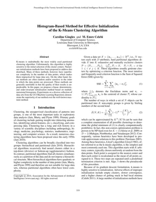
Fig. 1 illustrates this recursive algorithm on a two-
dimensional toy data set. The algorithm first scans the uni-
dimensional bins in the horizontal direction. The vertical ar-
1
Note that a unidimensional bin is in fact a stack of multidi-
mensional bins.
334

3. Figure 1: Illustration of the histogram traversal algorithm
row in panel (a) points to the most populated unidimensional
bin found in this first pass. The algorithm then scans this
unidimensional bin in the vertical direction. The horizontal
arrow in panel (b) points to the most populated bin found in
this second pass. Finally, the centroid of this bin, shown in
panel (c), is taken as the first cluster center.
It should be noted that the aforementioned algorithm re-
turns only one cluster center – that of the most populated
bin in the data set. In order to determine K centers, we
need execute this algorithm several times while preventing it
from simply returning previously selected multidimensional
bins. This can be accomplished by reducing the population
of each unidimensional bin at each step of the recursion.
The amount of reduction is determined based on the distance
between the geometric center (midpoint) of each unidimen-
sional bin and the centroids of the unidimensional bins cor-
responding to the previously selected centers. Let c be the
centroid of a unidimensional bin chosen at a certain step.
The population h+
of a unidimensional bin with geometric
center ˆc is reduced as follows:
h−
= h+
1 − exp −kD(ˆc − c)2
, (3)
where h−
is the reduced population of the unidimensional
bin in question and k is a tuning parameter. Since the pop-
ulation of the previously selected bin is vastly reduced, this
strongly steers the algorithm away from any previously se-
lected unidimensional bins. This also makes the algorithm
much less likely to pick bins very near to one another and
therefore likely to be in the same cluster. Note that this pop-
ulation reduction is cumulative. In other words, every time
the algorithm finds a cluster center, it reduces the population
of all unidimensional bins by an amount inversely propor-
tional to their distances to the selected unidimensional bin.
In this study, we used the following popular bin width
estimation rules2
: Scott (Scott 1979), Freedman–Diaconis
(Freedman and Diaconis 1981), Silverman (Silverman 1986,
p. 48), and Terrell (Terrell 1990). Table 1 gives the mathe-
matical formulae for these rules. Here, n, q, and s denote
2
The reader is referred to Sheather (Sheather 2004) and Heiden-
reich et al. (Heidenreich, Schindler, and Sperlich 2013) for recent
surveys on density estimation.
Table 1: Bin Width Estimation Formulae
Rule Formula k
Scott 3.49 s n−1/3
8.52
Freedman–Diaconis 2 q n−1/3
2.11
Silverman 0.9 min s,
q
1.34
n−1/5
2.51
Terrell 1.144 s n−1/5
9.71
Table 2: Descriptions of the Data Sets (N: # points, D: #
attributes, ˆK: # classes)
ID Data Set N D ˆK
1 Ecoli 336 7 8
2 Ionosphere 351 34 2
3 Iris (Bezdek) 150 4 3
4 Landsat Satellite (Statlog) 6,435 36 6
5 (Image) Segmentation 2,310 19 7
6 Shuttle (Statlog) 58,000 9 7
7 Vehicle Silhouettes (Statlog) 846 18 4
8 Wine Quality 6,497 11 7
the size, interquartile range3
, and standard deviation of the
sample. The last column gives the empirically determined
values for the tuning parameter used in Eq. (3). It should be
noted that, on a larger collection of data sets, we have deter-
mined that the optimal range of k values for each bin width
estimator is quite narrow.
Let x1, . . . , xN be the values of a particular attribute. The
number of bins for this attribute is calculated as follows:
b =
max{x1, . . . , xN } − min{x1, . . . , xN }
w
, (4)
where w is the bin width estimate given by one of the afore-
mentioned rules and y is the ceiling function, which gives
the smallest integer not less than y.
3 Experimental Results
The experiments were performed on eight commonly used
data sets from the UCI Machine Learning Repository (Frank
and Asuncion 2013). Table 2 gives the data set descriptions.
For each data set, the number of clusters (K) was set equal
to the number of classes ( ˆK), as commonly seen in the re-
lated literature (Bradley and Fayyad 1998; Arthur and Vas-
silvitskii 2007; Su and Dy 2007; Celebi and Kingravi 2012;
Celebi, Kingravi, and Vela 2013).
In clustering applications, normalization is a common
preprocessing step that is necessary to prevent attributes
with large ranges from dominating the distance calculations
and also to avoid numerical instabilities in the computations.
Two commonly used normalization schemes are linear scal-
ing to unit range (min-max normalization) and linear scal-
ing to unit variance (z-score normalization). In general, the
former scheme is preferable to the latter since the latter is
3
Interquartile range is defined as the difference between the up-
per and lower quartiles.
335

4. likely to eliminate valuable between-cluster variation (Mil-
ligan and Cooper 1988). For this reason, we used min-max
normalization to map the attributes of each data set to the
[0, 1] interval.
The convergence of k-means was controlled by the
disjunction of two criteria: the number of iterations
reaches a maximum of 100 or the relative improve-
ment in SSE between two consecutive iterations drops
below a threshold (Linde, Buzo, and Gray 1980), i.e.,
(SSEi−1 − SSEi) /SSEi ≤ , where SSEi is the SSE value
at the end of the ith (i ∈ {1, . . . , 100}) iteration. The con-
vergence threshold was set to = 10−6
.
The proposed histogram-based initialization method is
compared to the commonly used maximin initialization
method (Gonzalez 1985). This method chooses the first cen-
ter c1 arbitrarily and the remaining (K − 1) centers are cho-
sen successively as follows. In iteration i (i ∈ {2, . . . , K}),
the ith center ci is chosen as the point with the greatest min-
imum 2 distance to the previously selected (i − 1) centers,
i.e., c1, . . . , ci−1. This method can be expressed in algorith-
mic notation as follows:
1. Choose the first center c1 arbitrarily from the data points.
2. Choose the next center ci (i ∈ {2, . . . , K}) as the point
xˆ that satisfies
ˆ = arg max
j∈{1,...,N}
min
k∈{1,...,i−1}
xj − ck
2
2 . (5)
3. Repeat step #2 (K − 1) times.
Despite the fact that it was originally developed as a 2-
approximation to the K-center clustering problem4
, max-
imin is commonly used as a k-means initializer. In this study,
the first center is chosen as the centroid of X given by
¯x =
1
N
N
j=1
xj (6)
It is easy to see that c1 = ¯x gives the optimal SSE when
K = 1.
It should be noted that, in this study, we do not attempt
to compare a mixture of deterministic and random initial-
ization methods. Instead, we focus on deterministic meth-
ods for two main reasons. First, these methods are generally
computationally more efficient as they need to be executed
only once. In contrast, random methods are inherently un-
reliable in that the quality of their results is unpredictable
and thus it is common practice to perform multiple runs of
such methods and take the output of the run that produces
the least SSE. Second, several studies (Su and Dy 2007;
Celebi and Kingravi 2012; Celebi, Kingravi, and Vela 2013)
demonstrated that despite the fact that they are executed
4
Given a set of N points in a metric space, the goal of K-center
clustering is to find K representative points (centers) such that the
maximum distance of a point to a center is minimized (Har-Peled
2011, p. 63). Given a minimization problem, a 2-approximation
algorithm is one that finds a solution whose cost is at most twice
the cost of the optimal solution.
Table 3: SSE Comparison of the Initialization Methods
SSE
ID Method Initial Final
1
Maximin 47.9 19.3
Scott 36.5 18.5
Freedman–Diaconis 44.5 18.5
Silverman 44.2 18.6
Terrell 32.1 18.5
2
Maximin 826.5 826.5
Scott 1139.9 628.9
Freedman–Diaconis 913.1 628.9
Silverman 865.3 628.9
Terrell 986.3 628.9
3
Maximin 17.9 7.0
Scott 7.5 7.1
Freedman–Diaconis 14.5 7.0
Silverman 10.5 7.0
Terrell 13.5 7.1
4
Maximin 4815.9 1741.6
Scott 4926.6 1741.6
Freedman–Diaconis 2841.8 1741.6
Silverman 3073.3 1741.6
Terrell 5553.8 1741.6
5
Maximin 1084.5 433.3
Scott 833.9 387.0
Freedman–Diaconis 730.1 411.7
Silverman 636.8 387.0
Terrell 1045.4 414.7
6
Maximin 1817.8 725.8
Scott 792.1 235.0
Freedman–Diaconis 872.7 413.3
Silverman 1048.1 413.5
Terrell 1173.8 410.1
7
Maximin 466.0 237.7
Scott 320.7 223.5
Freedman–Diaconis 380.9 223.5
Silverman 463.1 237.5
Terrell 356.7 223.5
8
Maximin 732.6 399.4
Scott 671.7 348.6
Freedman–Diaconis 1085.8 334.5
Silverman 822.4 337.2
Terrell 626.0 346.8
Table 4: Rank Comparison of the Initialization Methods
SSE Rank
Method Initial Final
Maximin 4.00 4.63
Scott 2.38 2.44
Freedman–Diaconis 3.00 2.06
Silverman 2.63 2.81
Terrell 3.00 3.06
only once, some deterministic methods are highly competi-
tive with well-known and effective random methods such as
336

5. Bradley and Fayyad’s method (Bradley and Fayyad 1998)
and k-means++ (Arthur and Vassilvitskii 2007).
The performance of the initialization methods was quan-
tified using two effectiveness (quality) criteria:
Initial SSE: This is the SSE value calculated after the ini-
tialization phase, before the clustering phase. It gives us
a measure of the effectiveness of an initialization method
by itself.
Final SSE: This is the SSE value calculated after the clus-
tering phase. It gives us a measure of the effectiveness of
an initialization method when its output is refined by k-
means. Note that this is the objective function of the k-
means algorithm, i.e., Eq. (1).
Table 3 gives the initial and final SSE values for
the maximin method and the four variants (Scott,
Freedman–Diaconis, Silverman, and Terrell) of the proposed
histogram-based initialization method on the eight data sets.
The best (lowest) SSE values are shown in bold. It can
be seen that, with respect to initial SSE, variants of the
histogram-based initialization method outperform the max-
imin method by a large margin, except on data set # 2. This
means that in applications where an approximate clustering
of the data set is desired, one of the variants of the proposed
method can be used. There is significantly less variation
among the initialization methods with respect to final SSE
compared to initial SSE. In other words, the performance
of the initialization methods is more homogeneous with re-
spect to final SSE. This was expected because, being a local
optimization procedure, k-means can take two disparate ini-
tial configurations to similar (or, in some cases, even identi-
cal) local minima. Nevertheless, as the table shows, except
on data sets #3 and #4, variants of the histogram-based ini-
tialization method outperform the maximin method, in some
cases (e.g., data set #6), by a large margin.
We also ranked the initialization methods based on their
initial and final SSE values separately on each data set. In
case of ties, the tied ranks were given the mean of the rank
positions for which they are tied. For either effectiveness cri-
terion, an ideal method would attain a rank of 1. Table 4
gives these ranks averaged over all data sets. As expected,
there is no method that outperforms the rest consistently.
However, the maximin method ranks second-to-last (4.00)
and almost last (4.63) with respect to initial and final SSE,
respectively. In contrast, the proposed method attains the
best initial SSE rank (2.38) with Scott’s rule and the best
final SSE rank (2.06) with Freedman–Diaconis rule. Consid-
ering both effectiveness criteria simultaneously, the former
rule appears to be slightly better than the latter one.
4 Conclusions and Future Work
In this paper, we presented a novel, histogram-based ap-
proach to initialize the k-means clustering algorithm. The
method first normalizes the data set and then maps it to a
multidimensional histogram, where the bin width in each di-
mension is calculated using a rule-of-thumb estimator. In or-
der to determine the most populated K bins, this histogram
is then traversed using an efficient recursive algorithm. Fi-
nally, the centroids of these bins are taken as the initial
cluster centers. Besides being highly efficient, the proposed
method is deterministic, which means that it needs to be
executed only once prior to k-means. Experiments on a di-
verse collection of data sets from the UCI Machine Learning
Repository demonstrated the superiority of our method over
the popular maximin method. Future work includes testing
the proposed method on a larger collection of data sets us-
ing additional performance criteria and more sophisticated
bin width estimators.
5 Acknowledgments
This publication was made possible by a grant from the Na-
tional Science Foundation (1117457).
References
Aloise, D.; Deshpande, A.; Hansen, P.; and Popat, P. 2009.
NP-Hardness of Euclidean Sum-of-Squares Clustering. Ma-
chine Learning 75(2):245–248.
Arthur, D., and Vassilvitskii, S. 2007. K-Means++: The Ad-
vantages of Careful Seeding. In Proceedings of the 18th An-
nual ACM-SIAM Symposium on Discrete Algorithms, 1027–
1035.
Bradley, P. S., and Fayyad, U. 1998. Refining Initial Points
for K-Means Clustering. In Proceedings of the 15th Inter-
national Conference on Machine Learning, 91–99.
Celebi, M. E., and Kingravi, H. 2012. Deterministic Initial-
ization of the K-Means Algorithm Using Hierarchical Clus-
tering. International Journal of Pattern Recognition and Ar-
tificial Intelligence 26(7):1250018.
Celebi, M. E.; Kingravi, H.; and Vela, P. A. 2013. A Com-
parative Study of Efficient Initialization Methods for the K-
Means Clustering Algorithm. Expert Systems with Applica-
tions 40(1):200–210.
Celebi, M. E. 2011. Improving the Performance of K-
Means for Color Quantization. Image and Vision Computing
29(4):260–271.
Frank, A., and Asuncion, A. 2013. UCI Machine Learn-
ing Repository. http://archive.ics.uci.edu/ml. University of
California, Irvine, School of Information and Computer Sci-
ences.
Freedman, D., and Diaconis, P. 1981. On the Histogram as
a Density Estimator: L2 Theory. Zeitschrift f¨ur Wahrschein-
lichkeitstheorie und Verwandte Gebiete 57(4):453–476.
Gonzalez, T. 1985. Clustering to Minimize the Maximum
Intercluster Distance. Theoretical Computer Science 38(2–
3):293–306.
Har-Peled, S. 2011. Geometric Approximation Algorithms.
American Mathematical Society.
Heidenreich, N. B.; Schindler, A.; and Sperlich, S. 2013.
Bandwidth Selection for Kernel Density Estimation: A Re-
view of Fully Automatic Selectors. AStA Advances in Sta-
tistical Analysis 97(4):403–433.
Jain, A. K.; Murty, M. N.; and Flynn, P. J. 1999. Data
Clustering: A Review. ACM Computing Surveys 31(3):264–
323.
337

6. Jain, A. K. 2010. Data Clustering: 50 Years Beyond K-
means. Pattern Recognition Letters 31(8):651–666.
Linde, Y.; Buzo, A.; and Gray, R. 1980. An Algorithm for
Vector Quantizer Design. IEEE Transactions on Communi-
cations 28(1):84–95.
Lloyd, S. 1982. Least Squares Quantization in PCM. IEEE
Transactions on Information Theory 28(2):129–136.
Mahajan, M.; Nimbhorkar, P.; and Varadarajan, K. 2012.
The Planar k-Means Problem is NP-hard. Theoretical Com-
puter Science 442:13–21.
Milligan, G., and Cooper, M. C. 1988. A Study of Standard-
ization of Variables in Cluster Analysis. Journal of Classifi-
cation 5(2):181–204.
Scott, D. W. 1979. On Optimal and Data-Based Histograms.
Biometrika 66(3):605–610.
Scott, D. W. 1992. Multivariate Density Estimation: Theory,
Practice, and Visualization. John Wiley & Sons.
Sheather, S. J. 2004. Density Estimation. Statistical Science
19(4):588–597.
Silverman, B. W. 1986. Density Estimation for Statistics
and Data Analysis. Chapman and Hall/CRC.
Su, T., and Dy, J. G. 2007. In Search of Deterministic Meth-
ods for Initializing K-Means and Gaussian Mixture Cluster-
ing. Intelligent Data Analysis 11(4):319–338.
Tarsitano, A. 2003. A Computational Study of Several Re-
location Methods for K-Means Algorithms. Pattern Recog-
nition 36(12):2955–2966.
Terrell, G. R. 1990. The Maximal Smoothing Principle in
Density Estimation. Journal of the American Statistical As-
sociation 85(410):470–477.
338