Direct current circuits

P U Z Z L E R
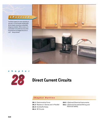
If all these appliances were operating at
one time, a circuit breaker would proba-
bly be tripped, preventing a potentially
dangerous situation. What causes a cir-
cuit breaker to trip when too many elec-
trical devices are plugged into one cir-
cuit? (George Semple)

c h a p t e r

Direct Current Circuits

Chapter Outline

28.1 Electromotive Force 28.5 (Optional) Electrical Instruments
28.2 Resistors in Series and in Parallel 28.6 (Optional) Household Wiring and
28.3 Kirchhoff’s Rules Electrical Safety
28.4 RC Circuits

868

28.1 Electromotive Force 869

T his chapter is concerned with the analysis of some simple electric circuits that
contain batteries, resistors, and capacitors in various combinations. The analysis
of these circuits is simpliﬁed by the use of two rules known as Kirchhoff’s rules,
which follow from the laws of conservation of energy and conservation of electric
charge. Most of the circuits analyzed are assumed to be in steady state, which means
that the currents are constant in magnitude and direction. In Section 28.4 we dis-
cuss circuits in which the current varies with time. Finally, we describe a variety of
common electrical devices and techniques for measuring current, potential differ-
ence, resistance, and emf.

28.1 ELECTROMOTIVE FORCE
In Section 27.6 we found that a constant current can be maintained in a closed cir-
cuit through the use of a source of emf, which is a device (such as a battery or gen-
erator) that produces an electric ﬁeld and thus may cause charges to move around
a circuit. One can think of a source of emf as a “charge pump.” When an electric
potential difference exists between two points, the source moves charges “uphill”
from the lower potential to the higher. The emf ␧
describes the work done per
unit charge, and hence the SI unit of emf is the volt.
Consider the circuit shown in Figure 28.1, consisting of a battery connected to
a resistor. We assume that the connecting wires have no resistance. The positive
terminal of the battery is at a higher potential than the negative terminal. If we ne-
glect the internal resistance of the battery, the potential difference across it (called
the terminal voltage) equals its emf. However, because a real battery always has some
internal resistance r, the terminal voltage is not equal to the emf for a battery in a
circuit in which there is a current. To understand why this is so, consider the cir-
cuit diagram in Figure 28.2a, where the battery of Figure 28.1 is represented by
the dashed rectangle containing an emf ␧
in series with an internal resistance r.
Now imagine moving through the battery clockwise from a to b and measuring the
electric potential at various locations. As we pass from the negative terminal to the
␧
positive terminal, the potential increases by an amount . However, as we move
through the resistance r, the potential decreases by an amount Ir, where I is the cur-
rent in the circuit. Thus, the terminal voltage of the battery ⌬V ϭ V b Ϫ V a is1

Battery
–
+

Figure 28.1 A circuit consisting of a resistor con-
Resistor nected to the terminals of a battery.

1 The terminal voltage in this case is less than the emf by an amount Ir. In some situations, the terminal
voltage may exceed the emf by an amount Ir. This happens when the direction of the current is opposite
that of the emf, as in the case of charging a battery with another source of emf.

870 CHAPTER 28 Direct Current Circuits

ε r ⌬V ϭ ␧ Ϫ Ir (28.1)
␧
a – + b
From this expression, note that is equivalent to the open-circuit voltage — that
is, the terminal voltage when the current is zero. The emf is the voltage labeled on a
I I battery — for example, the emf of a D cell is 1.5 V. The actual potential difference
R between the terminals of the battery depends on the current through the battery,
d c
as described by Equation 28.1.
(a)
Figure 28.2b is a graphical representation of the changes in electric potential
as the circuit is traversed in the clockwise direction. By inspecting Figure 28.2a, we
see that the terminal voltage ⌬V must equal the potential difference across the ex-
V ε r R
ternal resistance R, often called the load resistance. The load resistor might be a
simple resistive circuit element, as in Figure 28.1, or it could be the resistance of
some electrical device (such as a toaster, an electric heater, or a lightbulb) con-
ε Ir
nected to the battery (or, in the case of household devices, to the wall outlet). The
resistor represents a load on the battery because the battery must supply energy to
IR
operate the device. The potential difference across the load resistance is ⌬V ϭ IR .
Combining this expression with Equation 28.1, we see that
␧ ϭ IR ϩ Ir (28.2)
a b c d
Solving for the current gives
␧
(b)

Figure 28.2 (a) Circuit diagram Iϭ (28.3)
Rϩr
of a source of emf ␧ (in this case, a
battery), of internal resistance r, This equation shows that the current in this simple circuit depends on both the
connected to an external resistor of
load resistance R external to the battery and the internal resistance r. If R is much
resistance R. (b) Graphical repre-
sentation showing how the electric greater than r, as it is in many real-world circuits, we can neglect r.
potential changes as the circuit in If we multiply Equation 28.2 by the current I, we obtain
part (a) is traversed clockwise.
I ␧ ϭ I 2R ϩ I 2r (28.4)
This equation indicates that, because power ᏼ ϭ I ⌬V (see Eq. 27.22), the total
␧
power output I of the battery is delivered to the external load resistance in the
amount I 2R and to the internal resistance in the amount I 2r. Again, if r V R , then
most of the power delivered by the battery is transferred to the load resistance.

EXAMPLE 28.1 Terminal Voltage of a Battery
A battery has an emf of 12.0 V and an internal resistance of (b) Calculate the power delivered to the load resistor, the
0.05 ⍀. Its terminals are connected to a load resistance of power delivered to the internal resistance of the battery, and
3.00 ⍀. (a) Find the current in the circuit and the terminal the power delivered by the battery.
voltage of the battery.
Solution The power delivered to the load resistor is
Solution Using ﬁrst Equation 28.3 and then Equation
28.1, we obtain ᏼR ϭ I 2R ϭ (3.93 A)2 (3.00 ⍀) ϭ 46.3 W

Iϭ
␧ ϭ
12.0 V
ϭ 3.93 A The power delivered to the internal resistance is
Rϩr 3.05 ⍀
ᏼr ϭ I 2r ϭ (3.93 A)2 (0.05 ⍀) ϭ 0.772 W
⌬V ϭ ␧ Ϫ Ir ϭ 12.0 V Ϫ (3.93 A)(0.05 ⍀) ϭ 11.8 V
Hence, the power delivered by the battery is the sum of these
To check this result, we can calculate the voltage across the
quantities, or 47.1 W. You should check this result, using the
load resistance R :
expression ᏼ ϭ I . ␧
⌬V ϭ IR ϭ (3.93 A)(3.00 ⍀) ϭ 11.8 V

28.2 Resistors in Series and in Parallel 871

EXAMPLE 28.2 Matching the Load
Show that the maximum power delivered to the load resis- ᏼ
tance R in Figure 28.2a occurs when the load resistance
matches the internal resistance— that is, when R ϭ r . ᏼmax

Solution The power delivered to the load resistance is
equal to I 2R, where I is given by Equation 28.3:

ᏼ ϭ I 2R ϭ
␧2R
(R ϩ r)2
R
r 2r 3r
When ᏼ is plotted versus R as in Figure 28.3, we ﬁnd that ᏼ
␧
reaches a maximum value of 2/4r at R ϭ r. We can also Figure 28.3 Graph of the power ᏼ delivered by a battery to a load
prove this by differentiating ᏼ with respect to R , setting the resistor of resistance R as a function of R. The power delivered to the
result equal to zero, and solving for R . The details are left as resistor is a maximum when the load resistance equals the internal
a problem for you to solve (Problem 57). resistance of the battery.

28.2 RESISTORS IN SERIES AND IN PARALLEL
Suppose that you and your friends are at a crowded basketball game in a sports
arena and decide to leave early. You have two choices: (1) your whole group can
exit through a single door and walk down a long hallway containing several con-
cession stands, each surrounded by a large crowd of people waiting to buy food or
souvenirs; or (b) each member of your group can exit through a separate door in
the main hall of the arena, where each will have to push his or her way through a
single group of people standing by the door. In which scenario will less time be re-
quired for your group to leave the arena?
It should be clear that your group will be able to leave faster through the separate
doors than down the hallway where each of you has to push through several groups of
people. We could describe the groups of people in the hallway as acting in series, be-
cause each of you must push your way through all of the groups. The groups of peo-
ple around the doors in the arena can be described as acting in parallel. Each member
of your group must push through only one group of people, and each member
pushes through a different group of people. This simple analogy will help us under-
stand the behavior of currents in electric circuits containing more than one resistor.
When two or more resistors are connected together as are the lightbulbs in
Figure 28.4a, they are said to be in series. Figure 28.4b is the circuit diagram for the
lightbulbs, which are shown as resistors, and the battery. In a series connection, all
the charges moving through one resistor must also pass through the second resis-
tor. (This is analogous to all members of your group pushing through the crowds
in the single hallway of the sports arena.) Otherwise, charge would accumulate be-
tween the resistors. Thus,

for a series combination of resistors, the currents in the two resistors are the
same because any charge that passes through R 1 must also pass through R 2 .

The potential difference applied across the series combination of resistors will di-
vide between the resistors. In Figure 28.4b, because the voltage drop2 from a to b

2 The term voltage drop is synonymous with a decrease in electric potential across a resistor and is used

often by individuals working with electric circuits.


R1 R2

R1 R2 Req
a b c a c

+
–
I I
I

∆V ∆V
Battery + – + –

(a) (b) (c)

Figure 28.4 (a) A series connection of two resistors R 1 and R 2 . The current in R 1 is the same
as that in R 2 . (b) Circuit diagram for the two-resistor circuit. (c) The resistors replaced with a sin-
gle resistor having an equivalent resistance R eq ϭ R 1 ϩ R 2 .

equals IR1 and the voltage drop from b to c equals IR 2 , the voltage drop from a to
c is
⌬V ϭ IR 1 ϩ IR 2 ϭ I(R 1 ϩ R 2 )
Therefore, we can replace the two resistors in series with a single resistor having an
equivalent resistance Req , where
R eq ϭ R 1 ϩ R 2 (28.5)
The resistance R eq is equivalent to the series combination R 1 ϩ R 2 in the sense
that the circuit current is unchanged when R eq replaces R 1 ϩ R 2 .
The equivalent resistance of three or more resistors connected in series is

R eq ϭ R 1 ϩ R 2 ϩ R 3 ϩ иии (28.6)

This relationship indicates that the equivalent resistance of a series connec-
tion of resistors is always greater than any individual resistance.

Quick Quiz 28.1
If a piece of wire is used to connect points b and c in Figure 28.4b, does the brightness of
bulb R 1 increase, decrease, or stay the same? What happens to the brightness of bulb R 2 ?

Now consider two resistors connected in parallel, as shown in Figure 28.5.
When the current I reaches point a in Figure 28.5b, called a junction, it splits into
A series connection of three light- two parts, with I 1 going through R 1 and I 2 going through R 2 . A junction is any
bulbs, all rated at 120 V but having point in a circuit where a current can split ( just as your group might split up and
power ratings of 60 W, 75 W, and
200 W. Why are the intensities of leave the arena through several doors, as described earlier.) This split results in
the bulbs different? Which bulb less current in each individual resistor than the current leaving the battery. Be-
has the greatest resistance? How cause charge must be conserved, the current I that enters point a must equal the
would their relative intensities dif- total current leaving that point:
fer if they were connected in paral-
lel? I ϭ I1 ϩ I2


R1

R2

R1
R eq QuickLab
I1 Tape one pair of drinking straws end
+ R2 to end, and tape a second pair side by
–
a b side. Which pair is easier to blow
I2 I
through? What would happen if you
I were comparing three straws taped
∆V ∆V end to end with three taped side by
Battery + – + – side?

(a) (b) (c)

Figure 28.5 (a) A parallel connection of two resistors R 1 and R 2 . The potential difference
across R 1 is the same as that across R 2 . (b) Circuit diagram for the two-resistor circuit. (c) The
resistors replaced with a single resistor having an equivalent resistance R eq ϭ (R 1 Ϫ1 ϩ R 2 Ϫ1 )Ϫ1.

As can be seen from Figure 28.5, both resistors are connected directly across Straws in series
the terminals of the battery. Thus,

when resistors are connected in parallel, the potential differences across them
are the same. Straws in parallel

Because the potential differences across the resistors are the same, the expression
⌬V ϭ IR gives

I ϭ I1 ϩ I2 ϭ
⌬V
R1
ϩ
⌬V
R2
ϭ ⌬V ΂ R1
1
ϩ
1
R2 ΃ϭ R
⌬V
eq

From this result, we see that the equivalent resistance of two resistors in parallel is
given by
1 1 1
ϭ ϩ (28.7)
R eq R1 R2
or
1
R eq ϭ
1 1
ϩ
R1 R2
An extension of this analysis to three or more resistors in parallel gives

1 1 1 1
ϭ ϩ ϩ ϩ иии (28.8) The equivalent resistance of
R eq R1 R2 R3 several resistors in parallel


We can see from this expression that the equivalent resistance of two or more
resistors connected in parallel is always less than the least resistance in the
group.
Household circuits are always wired such that the appliances are connected in
parallel. Each device operates independently of the others so that if one is
switched off, the others remain on. In addition, the devices operate on the same
voltage.

Quick Quiz 28.2
Assume that the battery of Figure 28.1 has zero internal resistance. If we add a second resis-
tor in series with the first, does the current in the battery increase, decrease, or stay the
Three lightbulbs having power rat- same? How about the potential difference across the battery terminals? Would your answers
ings of 25 W, 75 W, and 150 W, change if the second resistor were connected in parallel to the first one?
connected in parallel to a voltage
source of about 100 V. All bulbs are
rated at the same voltage. Why do
the intensities differ? Which bulb
draws the most current? Which has Quick Quiz 28.3
the least resistance?
Are automobile headlights wired in series or in parallel? How can you tell?

EXAMPLE 28.3 Find the Equivalent Resistance
Four resistors are connected as shown in Figure 28.6a. I 2 ϭ 2.0 A. We could have guessed this at the start by noting
(a) Find the equivalent resistance between points a and c. that the current through the 3.0-⍀ resistor has to be twice that
through the 6.0-⍀ resistor, in view of their relative resistances
Solution The combination of resistors can be reduced in and the fact that the same voltage is applied to each of them.
steps, as shown in Figure 28.6. The 8.0-⍀ and 4.0-⍀ resistors As a final check of our results, note that ⌬V bc ϭ (6.0 ⍀)I 1 ϭ
are in series; thus, the equivalent resistance between a and b (3.0 ⍀)I 2 ϭ 6.0 V and ⌬V ab ϭ (12 ⍀)I ϭ 36 V; therefore,
is 12 ⍀ (see Eq. 28.5). The 6.0-⍀ and 3.0-⍀ resistors are in ⌬V ac ϭ ⌬V ab ϩ ⌬V bc ϭ 42 V, as it must.
parallel, so from Equation 28.7 we find that the equivalent re-
sistance from b to c is 2.0 ⍀. Hence, the equivalent resistance
6.0 Ω
from a to c is 14 ⍀.
I1
(b) What is the current in each resistor if a potential dif- 8.0 Ω 4.0 Ω
ference of 42 V is maintained between a and c ? (a) b
a I c
Solution The currents in the 8.0-⍀ and 4.0-⍀ resistors are I2
the same because they are in series. In addition, this is the
same as the current that would exist in the 14-⍀ equivalent 3.0 Ω
resistor subject to the 42-V potential difference. Therefore,
using Equation 27.8 (R ϭ ⌬V/I ) and the results from part
(a), we obtain
12 Ω 2.0 Ω
⌬V ac 42 V
Iϭ ϭ ϭ 3.0 A (b)
R eq 14 ⍀ a b c

This is the current in the 8.0-⍀ and 4.0-⍀ resistors. When this
3.0-A current enters the junction at b , however, it splits, with
part passing through the 6.0-⍀ resistor (I 1 ) and part through 14 Ω
the 3.0-⍀ resistor (I 2 ). Because the potential difference is ⌬Vbc (c)
across each of these resistors (since they are in parallel), we see a c
that (6.0 ⍀)I 1 ϭ (3.0 ⍀)I 2 , or I 2 ϭ 2I 1 . Using this result and
the fact that I 1 ϩ I 2 ϭ 3.0 A, we find that I 1 ϭ 1.0 A and Figure 28.6


EXAMPLE 28.4 Three Resistors in Parallel
Three resistors are connected in parallel as shown in Figure (c) Calculate the equivalent resistance of the circuit.
28.7. A potential difference of 18 V is maintained between
points a and b. (a) Find the current in each resistor. Solution We can use Equation 28.8 to ﬁnd R eq :
1 1 1 1
Solution The resistors are in parallel, and so the potential ϭ ϩ ϩ
difference across each must be 18 V. Applying the relation- R eq 3.0 ⍀ 6.0 ⍀ 9.0 ⍀
ship ⌬V ϭ IR to each resistor gives 6 3 2 11
ϭ ϩ ϩ ϭ
18 ⍀ 18 ⍀ 18 ⍀ 18 ⍀
⌬V 18 V
I1 ϭ ϭ ϭ 6.0 A
R1 3.0 ⍀ 18 ⍀
R eq ϭ ϭ 1.6 ⍀
11
⌬V 18 V
I2 ϭ ϭ ϭ 3.0 A
R2 6.0 ⍀
Exercise Use R eq to calculate the total power delivered by
⌬V 18 V the battery.
I3 ϭ ϭ ϭ 2.0 A
R3 9.0 ⍀
Answer 200 W.
(b) Calculate the power delivered to each resistor and the
total power delivered to the combination of resistors.
I
Solution We apply the relationship ᏼ ϭ (⌬V )2/R to each a
resistor and obtain
⌬V 2 (18 V )2 I1 I2 I3
ᏼ1 ϭ ϭ ϭ 110 W
R1 3.0 ⍀
⌬V 2 (18 V )2 18 V
ᏼ2 ϭ ϭ ϭ 54 W 3.0 Ω 6.0 Ω 9.0 Ω
R2 6.0 ⍀
⌬V 2 (18 V )2
ᏼ3 ϭ ϭ ϭ 36 W
R3 9.0 ⍀ b

This shows that the smallest resistor receives the most power. Figure 28.7 Three resistors connected in parallel. The voltage
Summing the three quantities gives a total power of 200 W. across each resistor is 18 V.

EXAMPLE 28.5 Finding Req by Symmetry Arguments
Consider ﬁve resistors connected as shown in Figure 28.8a. Solution In this type of problem, it is convenient to as-
Find the equivalent resistance between points a and b. sume a current entering junction a and then apply symmetry

5Ω

c

1Ω 1Ω 1Ω 1Ω
1/2 Ω 1/2 Ω 1Ω
5Ω
a b a c,d b a c,d b a b
1Ω 1Ω
1Ω 1Ω

d
(a) (b) (c) (d)

Figure 28.8 Because of the symmetry in this circuit, the 5-⍀ resistor does not contribute to the resistance between points a
and b and therefore can be disregarded when we calculate the equivalent resistance.


arguments. Because of the symmetry in the circuit (all 1-⍀ re- be removed from the circuit and the remaining circuit then
sistors in the outside loop), the currents in branches ac and reduced as in Figures 28.8c and d. From this reduction we see
ad must be equal; hence, the electric potentials at points c that the equivalent resistance of the combination is 1 ⍀. Note
and d must be equal. This means that ⌬V cd ϭ 0 and, as a re- that the result is 1 ⍀ regardless of the value of the resistor
sult, points c and d may be connected together without affect- connected between c and d.
ing the circuit, as in Figure 28.8b. Thus, the 5-⍀ resistor may

CONCEPTUAL EXAMPLE 28.6 Operation of a Three-Way Lightbulb
Figure 28.9 illustrates how a three-way lightbulb is con- Exercise Determine the resistances of the two filaments
structed to provide three levels of light intensity. The socket and their parallel equivalent resistance.
of the lamp is equipped with a three-way switch for selecting
different light intensities. The bulb contains two filaments. Answer 144 ⍀, 192 ⍀, 82.3 ⍀.
When the lamp is connected to a 120-V source, one filament
receives 100 W of power, and the other receives 75 W. Ex-
plain how the two filaments are used to provide three differ-
ent light intensities.

Solution The three light intensities are made possible by
applying the 120 V to one filament alone, to the other fila- 100-W filament
ment alone, or to the two filaments in parallel. When switch
S1 is closed and switch S2 is opened, current passes only
75-W filament
through the 75-W filament. When switch S1 is open and
switch S2 is closed, current passes only through the 100-W fil-
ament. When both switches are closed, current passes
through both filaments, and the total power is 175 W.
If the filaments were connected in series and one of them
were to break, no current could pass through the bulb, and S1
the bulb would give no illumination, regardless of the switch
position. However, with the filaments connected in parallel, if 120 V
S2
one of them (for example, the 75-W filament) breaks, the
bulb will still operate in two of the switch positions as current
passes through the other (100-W) filament. Figure 28.9 A three-way lightbulb.

APPLICATION Strings of Lights
Strings of lights are used for many ornamental purposes, In a parallel-wired string, each bulb operates at 120 V. By
such as decorating Christmas trees. Over the years, both par- design, the bulbs are brighter and hotter than those on a
allel and series connections have been used for multilight series-wired string. As a result, these bulbs are inherently
strings powered by 120 V.3 Series-wired bulbs are safer than more dangerous (more likely to start a fire, for instance), but
parallel-wired bulbs for indoor Christmas-tree use because if one bulb in a parallel-wired string fails or is removed, the
series-wired bulbs operate with less light per bulb and at a rest of the bulbs continue to glow. (A 25-bulb string of 4-W
lower temperature. However, if the filament of a single bulb bulbs results in a power of 100 W; the total power becomes
fails (or if the bulb is removed from its socket), all the lights substantial when several strings are used.)
on the string are extinguished. The popularity of series-wired A new design was developed for so-called “miniature”
light strings diminished because troubleshooting a failed lights wired in series, to prevent the failure of one bulb from
bulb was a tedious, time-consuming chore that involved trial- extinguishing the entire string. The solution is to create a
and-error substitution of a good bulb in each socket along connection (called a jumper) across the filament after it fails.
the string until the defective bulb was found. (If an alternate connection existed across the filament before
3 These and other household devices, such as the three-way lightbulb in Conceptual Example 28.6 and
the kitchen appliances shown in this chapter’s Puzzler, actually operate on alternating current (ac), to
be introduced in Chapter 33.

28.3 Kirchhoff’s Rules 877

it failed, each bulb would represent a parallel circuit; in this Suppose that all the bulbs in a 50-bulb miniature-light
circuit, the current would flow through the alternate connec- string are operating. A 2.4-V potential drop occurs across each
tion, forming a short circuit, and the bulb would not glow.) bulb because the bulbs are in series. The power input to this
When the filament breaks in one of these miniature light- style of bulb is 0.34 W, so the total power supplied to the
bulbs, 120 V appears across the bulb because no current is string is only 17 W. We calculate the filament resistance at
present in the bulb and therefore no drop in potential occurs the operating temperature to be (2.4 V)2/(0.34 W) ϭ 17 ⍀.
across the other bulbs. Inside the lightbulb, a small loop cov- When the bulb fails, the resistance across its terminals is re-
ered by an insulating material is wrapped around the fila- duced to zero because of the alternate jumper connection
ment leads. An arc burns the insulation and connects the fila- mentioned in the preceding paragraph. All the other bulbs
ment leads when 120 V appears across the bulb — that is, not only stay on but glow more brightly because the total resis-
when the filament fails. This “short” now completes the cir- tance of the string is reduced and consequently the current in
cuit through the bulb even though the filament is no longer each bulb increases.
active (Fig. 28.10). Let us assume that the operating resistance of a bulb re-
mains at 17 ⍀ even though its temperature rises as a result of
the increased current. If one bulb fails, the potential drop
across each of the remaining bulbs increases to 2.45 V, the
current increases from 0.142 A to 0.145 A, and the power in-
creases to 0.354 W. As more lights fail, the current keeps ris-
ing, the filament of each bulb operates at a higher tempera-
ture, and the lifetime of the bulb is reduced. It is therefore a
good idea to check for failed (nonglowing) bulbs in such a
series-wired string and replace them as soon as possible, in or-
der to maximize the lifetimes of all the bulbs.

Filament

Jumper

Figure 28.10 (a) Schematic diagram of
Glass insulator a modern “miniature” holiday lightbulb,
with a jumper connection to provide a cur-
rent path if the filament breaks. (b) A
Christmas-tree lightbulb.
(a) (b)

28.3 KIRCHHOFF’S RULES
As we saw in the preceding section, we can analyze simple circuits using the ex-
13.4 pression ⌬V ϭ IR and the rules for series and parallel combinations of resistors.
Very often, however, it is not possible to reduce a circuit to a single loop. The pro-
cedure for analyzing more complex circuits is greatly simplified if we use two prin-
ciples called Kirchhoff ’s rules:

1. The sum of the currents entering any junction in a circuit must equal the
sum of the currents leaving that junction:

⌺ I in ϭ ⌺ I out (28.9)


2. The sum of the potential differences across all elements around any closed
circuit loop must be zero:

⌺
closed
⌬V ϭ 0 (28.10)
loop

Kirchhoff’s first rule is a statement of conservation of electric charge. All cur-
rent that enters a given point in a circuit must leave that point because charge can-
not build up at a point. If we apply this rule to the junction shown in Figure
28.11a, we obtain
Gustav Kirchhoff (1824– 1887) I1 ϭ I2 ϩ I3
Kirchhoff, a professor at Heidelberg,
Germany, and Robert Bunsen in- Figure 28.11b represents a mechanical analog of this situation, in which water
vented the spectroscope and founded flows through a branched pipe having no leaks. The flow rate into the pipe equals
the science of spectroscopy, which the total flow rate out of the two branches on the right.
we shall study in Chapter 40. They Kirchhoff’s second rule follows from the law of conservation of energy. Let us
discovered the elements cesium and
imagine moving a charge around the loop. When the charge returns to the start-
rubidium and invented astronomical
spectroscopy. Kirchhoff formulated ing point, the charge – circuit system must have the same energy as when the
another Kirchhoff’s rule, namely, “a charge started from it. The sum of the increases in energy in some circuit ele-
cool substance will absorb light of the ments must equal the sum of the decreases in energy in other elements. The po-
same wavelengths that it emits when tential energy decreases whenever the charge moves through a potential drop ϪIR
hot.” (AIP ESVA/W. F. Meggers Collection)
across a resistor or whenever it moves in the reverse direction through a source of
emf. The potential energy increases whenever the charge passes through a battery
from the negative terminal to the positive terminal. Kirchhoff’s second rule ap-
plies only for circuits in which an electric potential is defined at each point; this
criterion may not be satisfied if changing electromagnetic fields are present, as we
shall see in Chapter 31.
In justifying our claim that Kirchhoff’s second rule is a statement of conserva-
QuickLab tion of energy, we imagined carrying a charge around a loop. When applying this
Draw an arbitrarily shaped closed rule, we imagine traveling around the loop and consider changes in electric potential,
loop that does not cross over itself.
rather than the changes in potential energy described in the previous paragraph.
Label five points on the loop a, b, c, d,
and e, and assign a random number You should note the following sign conventions when using the second rule:
to each point. Now start at a and
• Because charges move from the high-potential end of a resistor to the low-
work your way around the loop, cal-
culating the difference between each potential end, if a resistor is traversed in the direction of the current, the
pair of adjacent numbers. Some of change in potential ⌬V across the resistor is ϪIR (Fig. 28.12a).
these differences will be positive, and • If a resistor is traversed in the direction opposite the current, the change in po-
some will be negative. Add the differ- tential ⌬V across the resistor is ϩ IR (Fig. 28.12b).
ences together, making sure you accu-
• If a source of emf (assumed to have zero internal resistance) is traversed in the
rately keep track of the algebraic
signs. What is the sum of the differ- direction of the emf (from Ϫ to ϩ), the change in potential ⌬V is ϩ ␧ (Fig.
ences all the way around the loop? 28.12c). The emf of the battery increases the electric potential as we move
through it in this direction.
• If a source of emf (assumed to have zero internal resistance) is traversed in the
direction opposite the emf (from ϩ to Ϫ), the change in potential ⌬V is Ϫ ␧
(Fig. 28.12d). In this case the emf of the battery reduces the electric potential as
we move through it.
Limitations exist on the numbers of times you can usefully apply Kirchhoff’s
rules in analyzing a given circuit. You can use the junction rule as often as you
need, so long as each time you write an equation you include in it a current that
has not been used in a preceding junction-rule equation. In general, the number
of times you can use the junction rule is one fewer than the number of junction


I2 I
I1
(a)
a b
∆V = –IR
I3
I
(a)
(b)
a b
∆V = +IR
Flow in
Flow out
ε
– +
(c)
∆V = +ε
a b

(b)

Figure 28.11 (a) Kirchhoff’s ε
junction rule. Conservation of + –
charge requires that all current en- (d)
∆V = –ε
a b
tering a junction must leave that
junction. Therefore, I 1 ϭ I 2 ϩ I 3 .
(b) A mechanical analog of the Figure 28.12 Rules for determin-
junction rule: the amount of water ing the potential changes across a
ﬂowing out of the branches on the resistor and a battery. (The battery
right must equal the amount ﬂow- is assumed to have no internal re-
ing into the single branch on the sistance.) Each circuit element is
left. traversed from left to right.

points in the circuit. You can apply the loop rule as often as needed, so long as a
new circuit element (resistor or battery) or a new current appears in each new
equation. In general, in order to solve a particular circuit problem, the num-
ber of independent equations you need to obtain from the two rules equals
the number of unknown currents.
Complex networks containing many loops and junctions generate great num-
bers of independent linear equations and a correspondingly great number of un-
knowns. Such situations can be handled formally through the use of matrix alge-
bra. Computer programs can also be written to solve for the unknowns.
The following examples illustrate how to use Kirchhoff’s rules. In all cases, it is
assumed that the circuits have reached steady-state conditions — that is, the cur-
rents in the various branches are constant. Any capacitor acts as an open circuit;
that is, the current in the branch containing the capacitor is zero under steady-
state conditions.

Problem-Solving Hints
Kirchhoff’s Rules
• Draw a circuit diagram, and label all the known and unknown quantities.
You must assign a direction to the current in each branch of the circuit. Do
not be alarmed if you guess the direction of a current incorrectly; your re-
sult will be negative, but its magnitude will be correct. Although the assignment
of current directions is arbitrary, you must adhere rigorously to the assigned
directions when applying Kirchhoff’s rules.
• Apply the junction rule to any junctions in the circuit that provide new rela-
tionships among the various currents.


• Apply the loop rule to as many loops in the circuit as are needed to solve for
the unknowns. To apply this rule, you must correctly identify the change in
potential as you imagine crossing each element in traversing the closed loop
(either clockwise or counterclockwise). Watch out for errors in sign!
• Solve the equations simultaneously for the unknown quantities.

EXAMPLE 28.7 A Single-Loop Circuit
A single-loop circuit contains two resistors and two batteries, ⌺ ⌬V ϭ 0
as shown in Figure 28.13. (Neglect the internal resistances of
the batteries.) (a) Find the current in the circuit.
␧1 Ϫ IR 1 Ϫ ␧2 Ϫ IR 2 ϭ 0
Solving for I and using the values given in Figure 28.13, we
Solution We do not need Kirchhoff’s rules to analyze this obtain
simple circuit, but let us use them anyway just to see how they
are applied. There are no junctions in this single-loop circuit; Iϭ
␧1 Ϫ ␧2 ϭ
6.0 V Ϫ 12 V
ϭ Ϫ0.33 A
thus, the current is the same in all elements. Let us assume R1 ϩ R2 8.0 ⍀ ϩ 10 ⍀
that the current is clockwise, as shown in Figure 28.13. Tra- The negative sign for I indicates that the direction of the cur-
versing the circuit in the clockwise direction, starting at a, we rent is opposite the assumed direction.
␧
see that a : b represents a potential change of ϩ 1 , b : c (b) What power is delivered to each resistor? What power
represents a potential change of ϪIR 1 , c : d represents a po- is delivered by the 12-V battery?
␧
tential change of Ϫ 2 , and d : a represents a potential
change of ϪIR 2 . Applying Kirchhoff’s loop rule gives Solution
ᏼ1 ϭ I 2R 1 ϭ (0.33 A)2(8.0 ⍀) ϭ 0.87 W
ε 1 = 6.0 V
a
– + I
b ᏼ2 ϭ I 2R 2 ϭ (0.33 A)2(10 ⍀) ϭ 1.1 W
Hence, the total power delivered to the resistors is
ᏼ1 ϩ ᏼ2 ϭ 2.0 W.
R 2 = 10 Ω R 1 = 8.0 Ω ␧
The 12-V battery delivers power I 2 ϭ 4.0 W. Half of this
power is delivered to the two resistors, as we just calculated.
The other half is delivered to the 6-V battery, which is being
d c charged by the 12-V battery. If we had included the internal
– +
ε 2 = 12 V resistances of the batteries in our analysis, some of the power
would appear as internal energy in the batteries; as a result,
Figure 28.13 A series circuit containing two batteries and two re- we would have found that less power was being delivered to
sistors, where the polarities of the batteries are in opposition. the 6-V battery.

EXAMPLE 28.8 Applying Kirchhoff’s Rules
Find the currents I 1 , I 2 , and I 3 in the circuit shown in Figure We now have one equation with three unknowns — I 1 , I 2 , and
28.14. I3 . There are three loops in the circuit — abcda, befcb, and
aefda. We therefore need only two loop equations to deter-
Solution Notice that we cannot reduce this circuit to a mine the unknown currents. (The third loop equation would
simpler form by means of the rules of adding resistances in give no new information.) Applying Kirchhoff’s loop rule to
series and in parallel. We must use Kirchhoff’s rules to ana- loops abcda and befcb and traversing these loops clockwise, we
lyze this circuit. We arbitrarily choose the directions of the obtain the expressions
currents as labeled in Figure 28.14. Applying Kirchhoff’s
junction rule to junction c gives (2) abcda 10 V Ϫ (6 ⍀)I 1 Ϫ (2 ⍀)I 3 ϭ 0

(1) I1 ϩ I2 ϭ I3 (3) befcb Ϫ 14 V ϩ (6 ⍀)I 1 Ϫ 10 V Ϫ (4 ⍀)I 2 ϭ 0


Note that in loop befcb we obtain a positive value when travers- (5) Ϫ12 V ϭ Ϫ(3 ⍀)I 1 ϩ (2 ⍀)I 2
ing the 6-⍀ resistor because our direction of travel is opposite
Subtracting Equation (5) from Equation (4) eliminates I 2 ,
the assumed direction of I 1 .
giving
Expressions (1), (2), and (3) represent three independent
equations with three unknowns. Substituting Equation (1) 22 V ϭ (11 ⍀)I 1
into Equation (2) gives
10 V Ϫ (6 ⍀)I 1 Ϫ (2 ⍀) (I 1 ϩ I 2 ) ϭ 0 I1 ϭ 2 A

(4) 10 V ϭ (8 ⍀)I 1 ϩ (2 ⍀)I 2 Using this value of I 1 in Equation (5) gives a value for I 2 :
Dividing each term in Equation (3) by 2 and rearranging (2 ⍀)I 2 ϭ (3 ⍀)I 1 Ϫ 12 V ϭ (3 ⍀) (2 A) Ϫ 12 V ϭ Ϫ6 V
gives
I 2 ϭ Ϫ3 A

14 V Finally,
e + – f
I 3 ϭ I 1 ϩ I 2 ϭ Ϫ1 A
4Ω
I2 The fact that I 2 and I 3 are both negative indicates only that
– + I1 the currents are opposite the direction we chose for them.
b c
However, the numerical values are correct. What would have
6Ω I3
10 V happened had we left the current directions as labeled in Fig-
ure 28.14 but traversed the loops in the opposite direction?

a d
Exercise Find the potential difference between points b
2Ω and c.

Figure 28.14 A circuit containing three loops. Answer 2 V.

EXAMPLE 28.9 A Multiloop Circuit
(a) Under steady-state conditions, ﬁnd the unknown currents 4.00 V
I2 ϭ Ϫ ϭ Ϫ0.364 A
I 1 , I 2 , and I 3 in the multiloop circuit shown in Figure 28.15. 11.0 ⍀

Solution First note that because the capacitor represents Because our value for I 2 is negative, we conclude that the di-
an open circuit, there is no current between g and b along rection of I 2 is from c to f through the 3.00-⍀ resistor. Despite
path ghab under steady-state conditions. Therefore, when the 4.00 V
charges associated with I 1 reach point g, they all go through
d e
the 8.00-V battery to point b; hence, I gb ϭ I 1 . Labeling the
– +

currents as shown in Figure 28.15 and applying Equation 28.9 I3 5.00 Ω I3
to junction c, we obtain
3.00 Ω
(1) I 1 ϩ I 2 ϭ I 3 c f

Equation 28.10 applied to loops defcd and cfgbc, traversed I2
I1 5.00 Ω I1
clockwise, gives
(2) defcd 4.00 V Ϫ (3.00 ⍀)I 2 Ϫ (5.00 ⍀)I 3 ϭ 0 b + – g
(3) cfgbc (3.00 ⍀)I 2 Ϫ (5.00 ⍀)I 1 ϩ 8.00 V ϭ 0 8.00 V
I=0
From Equation (1) we see that I 1 ϭ I 3 Ϫ I 2 , which, when + –
substituted into Equation (3), gives a – + h
(4) (8.00 ⍀)I 2 Ϫ (5.00 ⍀)I 3 ϩ 8.00 V ϭ 0 3.00 V 6.00 µ F

Subtracting Equation (4) from Equation (2), we eliminate I 3 Figure 28.15 A multiloop circuit. Kirchhoff’s loop rule can be ap-
and ﬁnd that plied to any closed loop, including the one containing the capacitor.


this interpretation of the direction, however, we must con- Because Q ϭ C ⌬V cap (see Eq. 26.1), the charge on the capac-
tinue to use this negative value for I 2 in subsequent calcula- itor is
tions because our equations were established with our origi-
nal choice of direction. Q ϭ (6.00 ␮F)(11.0 V) ϭ 66.0 ␮C
Using I 2 ϭ Ϫ0.364 A in Equations (3) and (1) gives
Why is the left side of the capacitor positively charged?
I 1 ϭ 1.38 A I 3 ϭ 1.02 A
Exercise Find the voltage across the capacitor by traversing
(b) What is the charge on the capacitor? any other loop.
Solution We can apply Kirchhoff’s loop rule to loop bghab
(or any other loop that contains the capacitor) to find the po- Answer 11.0 V.
tential difference ⌬Vcap across the capacitor. We enter this po-
tential difference in the equation without reference to a sign Exercise Reverse the direction of the 3.00-V battery and an-
convention because the charge on the capacitor depends swer parts (a) and (b) again.
only on the magnitude of the potential difference. Moving
clockwise around this loop, we obtain
Answer (a) I 1 ϭ 1.38 A, I 2 ϭ Ϫ0.364 A, I 3 ϭ 1.02 A;
Ϫ8.00 V ϩ ⌬V cap Ϫ 3.00 V ϭ 0 (b) 30 ␮C.
⌬V cap ϭ 11.0 V

28.4 RC CIRCUITS
So far we have been analyzing steady-state circuits, in which the current is con-
stant. In circuits containing capacitors, the current may vary in time. A circuit con-
taining a series combination of a resistor and a capacitor is called an RC circuit.

Charging a Capacitor
Let us assume that the capacitor in Figure 28.16 is initially uncharged. There is no
current while switch S is open (Fig. 28.16b). If the switch is closed at t ϭ 0, how-
ever, charge begins to flow, setting up a current in the circuit, and the capacitor
begins to charge.4 Note that during charging, charges do not jump across the ca-
pacitor plates because the gap between the plates represents an open circuit. In-
stead, charge is transferred between each plate and its connecting wire due to the
electric field established in the wires by the battery, until the capacitor is fully
charged. As the plates become charged, the potential difference across the capaci-
tor increases. The value of the maximum charge depends on the voltage of the
battery. Once the maximum charge is reached, the current in the circuit is zero
because the potential difference across the capacitor matches that supplied by the
battery.
To analyze this circuit quantitatively, let us apply Kirchhoff’s loop rule to the
circuit after the switch is closed. Traversing the loop clockwise gives

␧Ϫ q
C
Ϫ IR ϭ 0 (28.11)

where q/C is the potential difference across the capacitor and IR is the potential
4 In previous discussions of capacitors, we assumed a steady-state situation, in which no current was
present in any branch of the circuit containing a capacitor. Now we are considering the case before the
steady-state condition is realized; in this situation, charges are moving and a current exists in the wires
connected to the capacitor.

28.4 RC Circuits 883

Resistor

Capacitor R R

+ –q
– C I
+q
Switch

S S
Battery ε ε
(a) (b) t < 0 (c) t > 0

Figure 28.16 (a) A capacitor in series with a resistor, switch, and battery. (b) Circuit diagram
representing this system at time t Ͻ 0, before the switch is closed. (c) Circuit diagram at time
t Ͼ 0, after the switch has been closed.

difference across the resistor. We have used the sign conventions discussed earlier
␧
for the signs on and IR. For the capacitor, notice that we are traveling in the di-
rection from the positive plate to the negative plate; this represents a decrease in
potential. Thus, we use a negative sign for this voltage in Equation 28.11. Note that
q and I are instantaneous values that depend on time (as opposed to steady-state val-
ues) as the capacitor is being charged.
We can use Equation 28.11 to find the initial current in the circuit and the
maximum charge on the capacitor. At the instant the switch is closed (t ϭ 0), the
charge on the capacitor is zero, and from Equation 28.11 we find that the initial
current in the circuit I 0 is a maximum and is equal to

I0 ϭ
␧ (current at t ϭ 0) (28.12) Maximum current
R
At this time, the potential difference from the battery terminals appears entirely
across the resistor. Later, when the capacitor is charged to its maximum value Q ,
charges cease to flow, the current in the circuit is zero, and the potential differ-
ence from the battery terminals appears entirely across the capacitor. Substituting
I ϭ 0 into Equation 28.11 gives the charge on the capacitor at this time:
QϭC ␧ (maximum charge) (28.13) Maximum charge on the capacitor

To determine analytical expressions for the time dependence of the charge
and current, we must solve Equation 28.11 — a single equation containing two vari-
ables, q and I. The current in all parts of the series circuit must be the same. Thus,
the current in the resistance R must be the same as the current flowing out of and
into the capacitor plates. This current is equal to the time rate of change of the
charge on the capacitor plates. Thus, we substitute I ϭ dq /dt into Equation 28.11
and rearrange the equation:
dq
ϭ Ϫ
q ␧
dt R RC
To find an expression for q, we first combine the terms on the right-hand side:
dq
ϭ
C
Ϫ
q␧ϭϪ
qϪC ␧
dt RC RC RC


Now we multiply by dt and divide by q Ϫ C ␧ to obtain
dq 1
ϭϪ
qϪC ␧ RC
dt

Integrating this expression, using the fact that q ϭ 0 at t ϭ 0, we obtain

͵ 0
q

␧
dq
qϪC
ϭϪ
1
RC
͵
t

0
dt

q Ϫ C␧
ln ΂
ϪC ␧ ΃
t
ϭϪ
RC
From the definition of the natural logarithm, we can write this expression as
Charge versus time for a capacitor
being charged
q(t ) ϭ C ␧ (1 Ϫ e Ϫt/RC ) ϭ Q(1 Ϫ e Ϫt /RC ) (28.14)

where e is the base of the natural logarithm and we have made the substitution
␧
C ϭ Q from Equation 28.13.
We can find an expression for the charging current by differentiating Equa-
tion 28.14 with respect to time. Using I ϭ dq /dt, we find that

Current versus time for a charging
I(t ) ϭ
␧ e Ϫt /RC (28.15)
capacitor
R

Plots of capacitor charge and circuit current versus time are shown in Figure
28.17. Note that the charge is zero at t ϭ 0 and approaches the maximum value
␧
C as t : ϱ. The current has its maximum value I 0 ϭ /R at t ϭ 0 and decays ex- ␧
ponentially to zero as t : ϱ. The quantity RC, which appears in the exponents of
Equations 28.14 and 28.15, is called the time constant ␶ of the circuit. It repre-
sents the time it takes the current to decrease to 1/e of its initial value; that is, in a
time ␶, I ϭ e Ϫ1I 0 ϭ 0.368I 0 . In a time 2␶, I ϭ e Ϫ2I 0 ϭ 0.135I 0 , and so forth. Like-
wise, in a time ␶, the charge increases from zero to C (1 Ϫ e Ϫ1) ϭ 0.632C .␧ ␧
The following dimensional analysis shows that ␶ has the units of time:

[␶] ϭ [RC] ϭ ΄ ⌬V ϫ ⌬V ΅ ϭ ΄ Q /⌬t ΅ ϭ [⌬t] ϭ T
I
Q Q

q I

Cε
I0 I0 = ε
R
0.632 Cε τ =RC

0.368I0

t t
τ τ

(a) (b)

Figure 28.17 (a) Plot of capacitor charge versus time for the circuit shown in Figure 28.16. Af-
ter a time interval equal to one time constant ␶ has passed, the charge is 63.2% of the maximum
value C ␧. The charge approaches its maximum value as t approaches infinity. (b) Plot of current
versus time for the circuit shown in Figure 28.16. The current has its maximum value I 0 ϭ ␧ /R
at t ϭ 0 and decays to zero exponentially as t approaches infinity. After a time interval equal to
one time constant ␶ has passed, the current is 36.8% of its initial value.

28.4 RC Circuits 885

Because ␶ ϭ RC has units of time, the combination t /RC is dimensionless, as it
must be in order to be an exponent of e in Equations 28.14 and 28.15.
The energy output of the battery as the capacitor is fully charged is
␧ ␧
Q ϭ C 2. After the capacitor is fully charged, the energy stored in the capacitor
␧ ␧
is 1Q ϭ 1C 2, which is just half the energy output of the battery. It is left as a
2 2
problem (Problem 60) to show that the remaining half of the energy supplied by
the battery appears as internal energy in the resistor.

Discharging a Capacitor
Now let us consider the circuit shown in Figure 28.18, which consists of a capaci-
tor carrying an initial charge Q , a resistor, and a switch. The initial charge Q is
–Q
not the same as the maximum charge Q in the previous discussion, unless the dis- C R
charge occurs after the capacitor is fully charged (as described earlier). When the +Q
switch is open, a potential difference Q /C exists across the capacitor and there is
zero potential difference across the resistor because I ϭ 0. If the switch is closed S
at t ϭ 0, the capacitor begins to discharge through the resistor. At some time t t<0
during the discharge, the current in the circuit is I and the charge on the capaci- (a)
tor is q (Fig. 28.18b). The circuit in Figure 28.18 is the same as the circuit in Fig-
ure 28.16 except for the absence of the battery. Thus, we eliminate the emf ␧
from Equation 28.11 to obtain the appropriate loop equation for the circuit in
Figure 28.18: –q
C R I
q +q
Ϫ Ϫ IR ϭ 0 (28.16)
C
When we substitute I ϭ dq /dt into this expression, it becomes S
t>0
dq q
ϪR ϭ (b)
dt C
Figure 28.18 (a) A charged ca-
dq 1 pacitor connected to a resistor and
ϭϪ dt
q RC a switch, which is open at t Ͻ 0.
(b) After the switch is closed, a cur-
Integrating this expression, using the fact that q ϭ Q at t ϭ 0, gives rent that decreases in magnitude

͵ ͵
q t
with time is set up in the direction
dq 1 shown, and the charge on the ca-
ϭϪ dt
Q q RC 0 pacitor decreases exponentially
with time.
ln΂ Q ΃ ϭ Ϫ RC
q t

Charge versus time for a
q(t ) ϭ Qe Ϫt /RC (28.17) discharging capacitor

Differentiating this expression with respect to time gives the instantaneous current
as a function of time:

dq d Q Ϫt /RC Current versus time for a
I(t) ϭ ϭ (Qe Ϫt /RC ) ϭ Ϫ e (28.18) discharging capacitor
dt dt RC

where Q /RC ϭ I 0 is the initial current. The negative sign indicates that the cur-
rent direction now that the capacitor is discharging is opposite the current direc-
tion when the capacitor was being charged. (Compare the current directions in
Figs. 28.16c and 28.18b.) We see that both the charge on the capacitor and the
current decay exponentially at a rate characterized by the time constant ␶ ϭ RC.


CONCEPTUAL EXAMPLE 28.10 Intermittent Windshield Wipers
Many automobiles are equipped with windshield wipers that through a multiposition switch. As it increases with time, the
can operate intermittently during a light rainfall. How does voltage across the capacitor reaches a point at which it trig-
the operation of such wipers depend on the charging and dis- gers the wipers and discharges, ready to begin another charg-
charging of a capacitor? ing cycle. The time interval between the individual sweeps of
the wipers is determined by the value of the time constant.
Solution The wipers are part of an RC circuit whose time
constant can be varied by selecting different values of R

EXAMPLE 28.11 Charging a Capacitor in an RC Circuit
An uncharged capacitor and a resistor are connected in se- Exercise Calculate the charge on the capacitor and the cur-
ries to a battery, as shown in Figure 28.19. If ϭ 12.0 V, ␧ rent in the circuit after one time constant has elapsed.
C ϭ 5.00 ␮F, and R ϭ 8.00 ϫ 10 5 ⍀, find the time constant
of the circuit, the maximum charge on the capacitor, the Answer 37.9 ␮C, 5.52 ␮A.
maximum current in the circuit, and the charge and current
as functions of time. µ
q(µC)
60 Q = 60.0 µ
µC
Solution The time constant of the circuit is ␶ ϭ RC ϭ
(8.00 ϫ ⍀)(5.00 ϫ 10 Ϫ6 F ) ϭ 4.00 s. The maximum
10 5 50
␧
charge on the capacitor is Q ϭ C ϭ (5.00 ␮F)(12.0 V) ϭ 40 t =τ
60.0 ␮C. The maximum current in the circuit is 30
␧
I 0 ϭ /R ϭ (12.0 V)/(8.00 ϫ 10 5 ⍀) ϭ 15.0 ␮A. Using these 20
values and Equations 28.14 and 28.15, we find that
10
0 t (s)
q(t ) ϭ (60.0 ␮C)(1 Ϫ e Ϫt/4.00 s ) 0 1 2 3 4 5 6 7
(a)
µ
I(µA)
I(t ) ϭ (15.0 ␮A) e Ϫt/4.00 s
15 I 0 = 15.0 µ
µA
Graphs of these functions are provided in Figure 28.20.

10

t =τ
R
5

C t (s)
0
ε 0 1 2 3 4 5 6 7
(b)
+ – S
Figure 28.20 Plots of (a) charge versus time and (b) current ver-
Figure 28.19 The switch of this series RC circuit, open for times sus time for the RC circuit shown in Figure 28.19, with ϭ 12.0 V,␧
t Ͻ 0, is closed at t ϭ 0. R ϭ 8.00 ϫ 10 5 ⍀, and C ϭ 5.00 ␮F.

EXAMPLE 28.12 Discharging a Capacitor in an RC Circuit
Consider a capacitor of capacitance C that is being dis- Solution The charge on the capacitor varies with time ac-
charged through a resistor of resistance R, as shown in Figure cording to Equation 28.17, q(t ) ϭ Qe Ϫt /RC. To find the time
28.18. (a) After how many time constants is the charge on the it takes q to drop to one-fourth its initial value, we substitute
capacitor one-fourth its initial value? q(t ) ϭ Q /4 into this expression and solve for t :

28.5 Electrical Instruments 887

Q q2 (Q e Ϫt /RC )2 Q 2 Ϫ2t /RC
ϭ Qe Ϫt /RC Uϭ ϭ ϭ e ϭ U 0e Ϫ2t /RC
4 2C 2C 2C
1
4 ϭ e Ϫt /RC where U 0 ϭ Q 2/2C is the initial energy stored in the capaci-
Taking logarithms of both sides, we find tor. As in part (a), we now set U ϭ U 0/4 and solve for t :
U0
Ϫln 4 ϭ Ϫ
t ϭ U 0e Ϫ2t /RC
RC 4
1
4 ϭ e Ϫ2t /RC
t ϭ RC(ln 4) ϭ 1.39RC ϭ 1.39␶
Again, taking logarithms of both sides and solving for t gives
(b) The energy stored in the capacitor decreases with
time as the capacitor discharges. After how many time con- t ϭ 1RC(ln 4) ϭ 0.693RC ϭ 0.693␶
2
stants is this stored energy one-fourth its initial value?
Exercise After how many time constants is the current in
Solution Using Equations 26.11 (U ϭ Q 2/2C ) and 28.17, the circuit one-half its initial value?
we can express the energy stored in the capacitor at any time
t as Answer 0.693RC ϭ 0.693␶.

EXAMPLE 28.13 Energy Delivered to a Resistor
A 5.00-␮ F capacitor is charged to a potential difference of
800 V and then discharged through a 25.0-k⍀ resistor. How Energy ϭ ͵
0
ϱ
I 2 R dt ϭ ͵ ϱ

0
(I 0e Ϫt /RC )2 R dt
much energy is delivered to the resistor in the time it takes to
fully discharge the capacitor? To evaluate this integral, we note that the initial current I 0 is
␧
equal to /R and that all parameters except t are constant.
Solution We shall solve this problem in two ways. The first Thus, we find
way is to note that the initial energy in the circuit equals the
␧
energy stored in the capacitor, C 2/2 (see Eq. 26.11). Once
the capacitor is fully discharged, the energy stored in it is
(1) Energy ϭ
␧2
R
͵ϱ

0
e Ϫ2t/RC dt

zero. Because energy is conserved, the initial energy stored in This integral has a value of RC/2; hence, we find
the capacitor is transformed into internal energy in the resis-
␧
tor. Using the given values of C and , we find
Energy ϭ 1C
2 ␧2
which agrees with the result we obtained using the simpler
Energy ϭ 1 C
2 ␧2 ϭ 1(5.00 ϫ 10 Ϫ6 F)(800 V)2 ϭ
2 1.60 J approach, as it must. Note that we can use this second ap-
proach to find the total energy delivered to the resistor at any
The second way, which is more difficult but perhaps more time after the switch is closed by simply replacing the upper
instructive, is to note that as the capacitor discharges through limit in the integral with that specific value of t.
the resistor, the rate at which energy is delivered to the resis-
tor is given by I 2R, where I is the instantaneous current given Exercise Show that the integral in Equation (1) has the
by Equation 28.18. Because power is defined as the time rate value RC/2.
of change of energy, we conclude that the energy delivered to
the resistor must equal the time integral of I 2R dt:

Optional Section

28.5 ELECTRICAL INSTRUMENTS
The Ammeter
A device that measures current is called an ammeter. The current to be measured
must pass directly through the ammeter, so the ammeter must be connected in se-

Direct current circuits

Recommandé

Recommandé

Contenu connexe

Tendances

Tendances (20)

Similaire à Direct current circuits

Similaire à Direct current circuits (20)

Dernier

Dernier (20)

Direct current circuits