2. May 2016 v Volume 7(5) v Article e012102 v www.esajournals.org
FAIVRE ET AL.
complex, and consequently quantitative models
of the spatial patterns of fire risk remain highly
uncertain.
The relative importance of the physical factors
controlling large wildfires in Southern Califor-
nia has been vigorously debated. One school of
thought has argued that large fires are the result
of past fire suppression (Minnich 1983, Minnich
and Chou 1997, Goforth and Minnich 2007). This
perspective has emphasized the buildup of vege-
tation and detritus, which is thought to contrib-
ute to the development of large fires. A second
school of thought has emphasized the importance
of extreme weather (Davis and Michaelsen 1995,
Moritz 1997, 2003, Keeley and Fotheringham
2001, Keeley and Zedler 2009, Moritz et al. 2010).
The literature documenting the latter perspective
has noted that large fires often occur during brief
episodes, from September through January when
strong SantaAna winds blow out of Southern Cal-
ifornia’s eastern deserts and mountains (Moritz
et al. 2010, Peterson et al. 2011). Santa Ana winds
often exceed 60 km/h and relative humidity may
drop below 10%, resulting in fires that can spread
at rates exceeding 10,000 ha/h (Keane et al. 2008).
Fire spread during these extreme conditions is of-
ten comparatively insensitive to landscape varia-
tions in fuel loads.Approximately, half of the total
burned area in Southern California occurs during
Santa Ana events; almost all of the remaining
burned area occurs during hot and dry summer
months when the winds are predominately on-
shore (Jin et al. 2014).
Unique sets of environmental factors may drive
the fire regime in the different ecoregions of Cal-
ifornia (Taylor and Skinner 2003, Stavros et al.
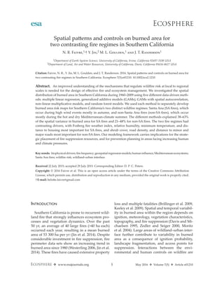
2014a,b). A conceptual diagram of the way physi-
cal and human factors interact to influence burned
area is shown in Fig. 1. Interactions between me-
teorology, fuel structure and composition, and the
frequency, spread, and severity of fire are well
known (Keeley and Fotheringham 2001, Mori-
tz 2003, Collins et al. 2007, Meyn et al. 2007, Ar-
chibald et al. 2009, Preisler et al. 2011, Parisien and
Moritz 2012). Within Southern California, fire sus-
ceptibility is known to be strongly related to va-
por pressure deficit and relative humidity, which
covary with attributes such as elevation and mean
annual precipitation (Parisien and Moritz 2012).
Human activity also exerts a strong influence on
fire frequency and burned area (Syphard et al.
2007). Variation in ignition frequency, for exam-
ple, is positively related to the extent of human de-
velopment and negatively related to the distance
from infrastructure such as housing and roads
(Syphard et al. 2008; Faivre et al. 2014). Roads also
Fig. 1. Conceptual model of the major factors controlling burned area in Southern California (adapted from
Archibald et al. 2009). The diagram categorizes the controls among human-related and biophysical variables and
shows how they relate to fire regime and influence burned area.
3. May 2016 v Volume 7(5) v Article e012103 v www.esajournals.org
FAIVRE ET AL.
may serve as a barrier to fire spread, particularly
for non-Santa Ana fires (Jin et al. 2015).
Three recent advances provide a foundation
for more accurately modeling fire risk in South-
ern California. First, increasing quality and avail-
ability of geographic information system data
sets describing human variables makes it pos-
sible to develop more sophisticated approaches
for representing the interactions between human
and environmental drivers shown in Fig. 1. Lim-
ited access to this type of information in previous
regional assessments in Southern California and
elsewhere may have led to an overreliance on
climate and weather drivers. Second, the use of
high resolution meteorology has made it possible
for the first time to quantitatively separate Santa
Ana and non-Santa Ana fires in the fire record
(Jin et al. 2014). This is important because the
way climate and other environmental variables
influence these two fire types is considerably
different (Jin et al. 2015). Third, new statistical
techniques have the potential to improve model
formulation and yield insight about the relation-
ship between driver variables. Ecological studies
comparing the predictive ability of regression
models to explain species distributions and fire
dynamics have shown considerable variation,
depending on methodology (Segurado and
Araujo 2004, Elith and Graham 2009, Syphard
and Franklin 2009). Prasad et al. (2006) concluded
that machine learning methods, such as random
forest or boosted regression trees, produce more
accurate results in ecological studies than linear
or additive models. Studies comparing multiple
regression to ensemble learning techniques such
as random forest modeling (Breiman 2001) for
burned area are currently lacking.
Here, we investigate the relationship between
burned area and human and biophysical con-
trols in Southern California using an array of
modeling techniques, including (1) multiple lin-
ear regression, (2) generalized additive models
(GAMs), (3) GAMs with spatial autocorrelation,
(4) non-linear multiplicative models, and (5)
random forest models. Our analysis focuses on
the spatial pattern of mean annual burned area
during 1960–2009, and begins by partitioning
this area into Santa Ana (SA) and non-Santa Ana
(non-SA) components (Jin et al. 2014). Our use of
multiple modeling approaches allowed us to test
the ability of each technique to accurately predict
the spatial pattern of burned area for both fire re-
gimes and to quantify the relative contribution of
the most important controls. Our analysis carries
implications for the effect of climate change and
further WUI development on Southern Califor-
nia fire risk, while also contributing to regional
assessments of fire risk and more effective strate-
gies for fire and ecosystem management.
Data and Methods
Study area
Our study domain spanned 36,500 km2 of
wildland and developed areas in Southern
California within Santa Barbara, Ventura, Los
Angeles, San Bernardino, Orange, Riverside
and San Diego counties. Southern California’s
Mediterranean-type climate is characterized by
a dry summer followed by a relatively brief
and mild rainy season (Bailey 1966). Spatial
gradients of temperature and rainfall result in
a variety of vegetation habitats (Franklin 1998).
Widespread vegetation types include chaparral
shrubland, coastal sage shrubland, valley grass-
land, open oak woodland, oak woodland, and
coniferous forest (Di Castri et al. 1981, Arroyo
et al. 1995, Davis and Richardson 1995).
Southern California has experienced intense
population pressure and urban growth around
the major metropolitan areas during the past
five decades; this has created widespread urban
communities interspersed with wildland areas
and connected by an extensive road network.
Over 22 million people lived in Southern
California in 2010 (source: US Census Bureau
2012). We focused our analysis on predicting
the regional burned area patterns throughout
Southern California after excluding dense urban
areas and deserts. Urban areas in the study
domain represented less than 8% of the total
land area, while the wildland–urban interface
(WUI) accounted for 17%. Two-thirds of the
area within the WUI consisted of housing in
the vicinity of contiguous wildland vegetation
and the remaining third was interspersed hous-
ing and vegetation.
Data sets: Wildfire data
We assessed burned area using the digitized
perimeter for all reported fires >40 ha compiled
by the California Department of Forestry – Fire
4. May 2016 v Volume 7(5) v Article e012104 v www.esajournals.org
FAIVRE ET AL.
and Resource Assessment Program (FRAP 2010).
We focused on the 50-yr period from 1960 to
2009; the fire records during this period were
more reliable than earlier records, and the pe-
riod overlapped with the availability of infor-
mation on human and biophysical factors.
We carried out our analysis at a 3 × 3 km res-
olution to match the spatial resolution of com-
plementary downscaled meteorological data sets
that were important for characterizing regional
variations in fire weather (Faivre et al. 2014). A
sensitivity test was done during a preliminary
analysis stage to quantify the effect of spatial
resolution. We found that the 3-km resolution
did not produce results that were systematical-
ly different from those using a finer resolution
of 1 km. The 3-km resolution resulted in a sam-
ple total of 3590 grid cells that had a large and
well-distributed range of burned area fractions,
which aided model development. We considered
burned area fraction, defined as the ratio of total
area burned summed during 1960–2009 within
each 3 × 3 km grid cell divided by the grid cell
area as the dependent variable. Multiple human
and environmental variables, which are de-
scribed below, were the predictors. The ArcGIS
overlay geoprocessing tool was used to intersect
the polygon layer of the grid cell boundaries with
all fire polygons during 1960–2009, and the areas
of all intersected new polygons within each indi-
vidual grid were then summed. For example, if
two different fires during the study period each
burned half of the grid area, the resulting burned
area fraction would be one. We classified the his-
toric record of fire perimeters into SA fires and
non-SA fires using the start date reported in the
FRAP database and a continuous historic time se-
ries of days with Santa Ana conditions (Jin et al.
2014, Fig. 2). Santa Ana days were determined
using a downscaled meteorological time series
that was obtained by driving the MM5 mesoscale
model with the ERA-40 and North American Re-
gional Reanalysis data sets. Santa Ana days were
identified when the northeasterly component
of the daily mean wind speed was greater than
6 m/s at the exit of the largest gap across the San-
ta Monica Mountains (Hughes and Hall 2010).
Data sets: Human factors
Humans can influence wildland fire regimes
through several different pathways (Hammer
et al. 2007, Radeloff et al. 2010). WUI areas
and road networks, for example, influence fuel
continuity, the patterns of ignition and access
for suppression (Lloret et al. 2002, Rollins et al.
2002, Ryu et al. 2007). We defined the WUI
as areas with less than 50% vegetation and at
least 6.2 houses/km2 (1 house per 40 acres)
that are located within 2.4 km of a 5 km2 (or
greater) area that is more than 75% vegetated
(Stewart et al. 2007).
We considered seven variables to describe
the human influence on burned area: (1) dis-
tance of cell center to a major road, (2) distance
of cell center to a minor road, (3) road density,
(4) population density, (5) distance of cell cen-
ter to low-density housing, (6) wildland–urban
land fragmentation, and (7) ignition frequency.
We derived these seven variables using the best
available statewide data. Geographic Encoding
and Referencing road data (TIGER; US Census
Bureau 2000) was used to calculate the road
density per grid cell and the distance to nearest
road from the cell centroid. We computed aver-
age population and housing density per 3 × 3 km
grid for 1960–2009 using the 1990 and 2000 U.S.
decennial census spatial data, along with consis-
tent decadal projections of past growth trends
for 1960, 1970, and 1980 (see Hammer et al. 2004,
2007 for details). We used the distance from cell
centroid to the nearest housing area with a den-
sity greater than 6.2 housing units/km2 as an in-
dicator of the proximity to low-density housing
within the WUI.
Wildland–urban land fragmentation was cal-
culated using an edge density metric that rep-
resented the degree of spatial heterogeneity in
the landscape. We used a land cover data set at
100 m resolution from the California Department
of Forestry and Fire Protection’s Fire Resource
Assessment Program (FRAP 2002) to aggregate
vector-based layers describing urban and non-
urban land cover types. The resulting binary
map was then processed using the FRAGSTATS
software package (McGarigal and Marks 1995) to
analyze the spatial arrangement of wildland–ur-
ban patterns. We tested several landscape met-
rics including the patch density, mean patch size,
mean shape index, edge density, mean nearest
neighbor distance between similar patches and
the interspersion and juxtaposition index (see
McGarigal and Marks 1995 for a definition of
5. May 2016 v Volume 7(5) v Article e012105 v www.esajournals.org
FAIVRE ET AL.
Fig. 2. Historical fire patterns in Southern California. The number of fires reported from 1960 to 2009 is
shown for Santa Ana fires (a) and non-Santa Ana fires (b).
6. May 2016 v Volume 7(5) v Article e012106 v www.esajournals.org
FAIVRE ET AL.
Fig. 3. Expanded map of the Cajon Pass section of the study area, including the 3 × 3 km grid overlay used to
analyze burned area. (a) The number of fires reported from 1960 to 2009. (b) The local land use/land cover. (c)
The local housing density and major and minor roads.
7. May 2016 v Volume 7(5) v Article e012107 v www.esajournals.org
FAIVRE ET AL.
metrics). We found that edge density was the
best proxy for quantifying the complexity of
wildland patches imbricated within urban areas.
Edge density (ED) is a shape index that indicates
whether the wildland–urban boundary is simple
and compact (low value) or irregular and convo-
luted (high value). We computed the mean for
each predictor within each 3 × 3 km grid cell by
Table 1. Spatial data on human and biophysical drivers of burned area used as inputs to the models.
Burned area drivers and
input variables Variable name Data resolution Data source
Human accessibility
Distance to major roads (km) d.majR 1:100,000 Census Bureau’s TIGER road data (Topologically
Integrated Geographic Encoding and
Referencing) (US Census 2000)
Distance to minor roads (km) d.minR 1:100,000 Census Bureau’s TIGER road data (Topologically
Integrated Geographic Encoding and
Referencing) (US Census Bureau 2000)
Distance to low-density
housing (km)
d.hou NA Census block-group data for 2000 (US Census
Bureau 2001)
Urban development
Population density
(Mpers./km2)
pop.den NA Census block-group data for 2000 (US Census
Bureau 2001)
Ignition frequency (No.
ignitions/km2)
pred.ign 3 km Ignition frequency estimates for Southern
California (Faivre et al. 2014)
Land fragmentation
Edge density index (0–100) ed.den 30 m WUI maps computed from the 1990 and 2000
US Census block datasets (Radeloff et al. 2005)
Road density (km roads/km2) rd.den 1:100,000 Census Bureau’s TIGER road data (Topologically
Integrated Geographic Encoding and
Referencing) (US Census Bureau 2000)
Topography
Elevation (m) elev 90 m Digital elevation data from the United States
Geological Survey—National Elevation Dataset
Slope (%) slope 90 m Digital elevation data from the United States
Geological Survey—National Elevation Dataset
Land cover
Tree cover (%) tree 100 m California Department of Forestry and Fire
Protection’s Fire Resource Assessment Program
(FRAP 2002)
Shrub cover (%) shrub 100 m California Department of Forestry and Fire
Protection’s Fire Resource Assessment Program
(FRAP 2002)
Grass cover (%) grass 100 m California Department of Forestry and Fire
Protection’s Fire Resource Assessment Program
(FRAP 2002)
Climate
Temperature maximum (°C) tmax 800 m Monthly estimates of average daily maximum
temperature from PRISM (Daly et al. 2008)
Temperature minimum (°C) tmin 800 m Monthly estimates of average daily minimum
temperature from PRISM (Daly et al. 2008)
Precipitation (mm/yr) prec 800 m Monthly estimates of mean cumulative
precipitation from PRISM (Daly et al. 2008)
Weather
Fosberg fire weather index ffwi 6 km Daily estimates of a mesoscale model version 5
(MM5)—Penn State/National Center for
Atmospheric Research
Relative humidity rel.h 6 km Daily estimates of a mesoscale model version 5
(MM5)—Penn State/National Center for
Atmospheric Research
Wind speed (m/s) wind.s 6 km Daily estimates of a mesoscale model version 5
(MM5)—Penn State/National Center for
Atmospheric Research
8. May 2016 v Volume 7(5) v Article e012108 v www.esajournals.org
FAIVRE ET AL.
applying the zonal statistics tool in ArcGIS Spa-
tial Analyst (Fig. 3).
Consistent region-wide ignition data outside of
the National Forests were unavailable, and we es-
timated ignition frequency for each 3 × 3 km grid
using the spatial modeling approach developed
in Faivre et al. (2014). Poisson regression analy-
ses were used to model ignition frequency as a
function of the dominant human and biophysical
covariates (Syphard et al. 2008, Faivre et al. 2014).
Data sets: Vegetation and biophysical factors
We used a set of 12 environmental variables
that were expected to influence the physical
characteristics of fuel, including continuity,
moisture, or loading (Fig. 1). These variables
can be sorted into three main categories: to-
pography (1-elevation, 2-slope), land cover (frac-
tional cover of 3-forest, 4-shrubland, 5-grassland,
and 6-other), and meteorology (annual average
daily 7-maximum and 8-minimum temperature,
9-cumulative winter precipitation, 10-wind
speed, 11-relative humidity, and 12-Fosberg fire
weather index (FFWI) (Table 1)). The FFWI is
a non-linear construct of meteorological condi-
tions (i.e., temperature, relative humidity, and
wind speed), which is widely used to infer
wildfire potential from the short-term weather
conditions (Fosberg 1978). FFWI values range
from 0 to 100; values ≥50 indicate a significant
threat of wildfire incidence and spread.
The topographic variables (elevation and
slope) were calculated for each 3 × 3 km grid
cell using the three arc-second digital elevation
model from the U.S. Geological Survey National
Elevation Dataset (NED). We assessed vegeta-
tion characteristics using the recent and compre-
hensive land cover data set at 100 m resolution
from the California Department of Forestry and
Fire Protection’s Fire Resource Assessment Pro-
gram (FRAP 2002). We classified the mixed veg-
etation of wildland areas into three major types:
“shrubland” (comprising 52% of the study area),
“forest/woodland” (19%), and “grassland” (8%).
The remaining non-vegetated land cover types
(21%) were grouped as “other”; this category in-
cluded agricultural land, urban, desert, wetland,
water, and barren soil. We calculated the frac-
tion of each class within each 3 × 3 km grid cell.
We derived several of the meteorological
variables from the monthly gridded Parameter-
Elevation Regressions on Independent Slopes
Model (PRISM) data set that has a native reso-
lution of 800 m (Daly et al. 2002; Oregon State
University PRISM Group). Winter precipitation
was estimated using monthly mean of precipita-
tion during September through March for each
3 × 3 km cell over the 1960–2009 period. Similarly,
variables representing the annual mean of daily
maximum temperature and the annual mean
of daily minimum temperature were calculated
over the period by averaging all the available
monthly files.
To capture the spatial pattern of meteorologi-
cal conditions that typically occur during SA and
non-SA fires, we estimated daily relative humid-
ity, wind speed, and the Fosberg Fire Weather
Index using 3-hourly model outputs from the
Mesoscale Model version 5 (MM5) forced with
reanalysis data sets as described by Jin et al.
(2014). Santa Ana days were identified using
winds at the exit of the largest gap in the San-
ta Monica Mountains (Hughes and Hall 2010).
Most of the Santa Ana events occurred in late
autumn and early winter in Southern California,
and most SAfires occurred in a 3-month window
from September to November (Jin et al. 2014).
We therefore quantified the meteorological con-
ditions that typically occur during SA fires by
averaging each of these three variables from the
MM5 daily time series during Santa Ana days
from September to November. For non-SA fires,
we calculated these same variables during non-
Santa Ana days from June to August. We resa-
mpled all meteorological data to the common
3 × 3 km grids.
Modeling approaches to predict burned area
We built, tested, and compared five modeling
approaches separately for SA and non-SA fires:
multiple linear regression (MLR), generalized
additive models (GAMs), GAMs incorporating
spatial autocorrelation (GAMspA), non-linear
multiplicative models (NMM), and random for-
est models (RF).
MLR has been used extensively to analyze
the relationship between burned area and en-
vironmental controls (Larsen 1996, Carvalho
et al. 2008, Camia and Amatulli 2009). Empirical
studies often predict a high proportion of the
variation in burned area using MLR (Flannigan
and Harrington 1988, Turner and Romme 1994,
9. May 2016 v Volume 7(5) v Article e012109 v www.esajournals.org
FAIVRE ET AL.
Turner et al. 1994, Larsen 1996). However, linear
regression assumes the variance of the response
variable is constant across observations and the
errors follow a normal (Gaussian) distribution;
these assumptions may be invalid for the estima-
tion of burned area or other ecological variables
(Viegas and Viegas 1994, Li et al. 1997, McCarthy
et al. 2001). We therefore also considered gener-
alized additive models (GAMs), which are com-
paratively flexible and often are better-suited for
analyzing ecological data based on non-linear
responses to predictor variables (Hastie and Tib-
shirani 1986).
These modeling approaches assume spatial sta-
tionarity (i.e., effects of environmental correlates
are constant across the region) and isotropic spa-
tial autocorrelation (i.e., the process resulting
in spatial autocorrelation acts in the same way
in all directions). Anisotropic spatial autocor-
relation arises when the variables of interest in
nearby sample units are not independent of each
other (Griffith 1987), i.e., in ecological data. Such
spatial patterns are usually explained by envi-
ronmental features such as climatic or habitat
structure variables that are themselves spatially
structured (e.g., directionality and intensity of
wind patterns). It is often impossible to measure
all spatially structured variables, and this issue
affects the uncertainty of statistical models (Leg-
endre 1993, Legendre et al. 2002). A positive spa-
tial autocorrelation (i.e., closer locations having
more similar residual values than others) tends
to underestimate the true standard error of pa-
rameters, which leads to an over estimation of
the regression coefficients.
We thus constructed a version of the GAM
model accounting for spatial autocorrelation to
better represent gradually changing spatial vari-
ability in environmental correlates. We imple-
mented these autocovariate GAMs by calculat-
ing locally weighed regressions within a moving
window spanning the entire study domain. We
included a two-dimensional smoothing function
f(xi,yi) in the GAMs, using the two geographic co-
ordinates (i.e., latitude and longitude) as a single
variable, along with the other terms in the model
(Wood and Augustin 2002, Wood 2003).
As an alternative approach to GAM, we in-
vestigated the use of non-linear multiplicative
regression models. Previous modeling studies
have shown that the rate of fire spread has a pos-
itive exponential relationship with slope (Junpen
et al. 2013) and fuel load (Cheney et al. 1998, Mar-
tins Fernandes 2001), and a negative exponential
relationship with fuel moisture content (Junpen
et al. 2013). Thus, we tested several non-linear
multiplicative models including power functions
(of the form y = xr), rational functions (quotients
of polynomial functions), exponential decay and
growth functions (Eq. 1), logistic functions (Eq.
2) and combined forms. We performed an opti-
mization of the model equations using the non-
linear least squares solver (nls; Bates and Watts
1988) that estimates iteratively the coefficients
of explanatory variables to find the best fit (i.e.,
highest correlation) with the response variable.
(1)
(2)
The previous modeling approaches are sensi-
tive to collinearity among predictors, which can
hinder the variable selection process, and mod-
el predictive power. A promising alternative is
the use of classification and regression tree tech-
niques; these approaches are generally more ro-
bust to the inclusion of correlated variables, and
are complementary to generalized linear and ad-
ditive models (Archer and Kimes 2008). Conse-
quently, we implemented a random forest mod-
el (R package “random forest”) by generating a
large number of bootstrapped trees (using a ran-
domized subset of predictors), and reserving 30%
of the data for testing (Breiman 2001). We trained
1000 trees using 70% of the data and selected six
predictors at each split. We used a default min-
imum node size of five to prevent the creation
of small sample nodes without increasing the
overall relative error (i.e., misclassification rate;
Breiman (2001)). The model predictions were ob-
tained using the reserved data each time a tree
was grown. The final predictions consisted of the
average of all predictions from the 1000 regres-
sion trees.
Variable selection and model validation
We performed initial univariate regressions
between the response variable and all predictors
f(x,𝜃)=𝜃1 × e−𝜃2x
f(x,𝜃)=
𝜃1
1+𝜃2 × e−𝜃3x
10. May 2016 v Volume 7(5) v Article e0121010 v www.esajournals.org
FAIVRE ET AL.
Table 2. Univariate impacts of various controls on spatial patterns of Santa Ana and non-SA fires using a linear
regression approach.
Explanatory variable
Santa Ana fires
Explanatory variable
non-Santa Ana fires
rpearson R2 rpearson R2
Fosberg Fire Weather Index 0.35 12.3% Shrub cover 0.34 11.5%
Relative Humidity −0.29 8.4% Road density −0.24 5.7%
Temperature minimum 0.28 7.8% Distance to minor roads 0.22 4.8%
Distance to Housing −0.28 7.8% Distance to major roads 0.19 3.6%
Wind Speed 0.25 6.2% Relative Humidity −0.19 3.6%
Elevation −0.25 6.2% Grass cover −0.16 2.6%
Shrub cover 0.23 5.3% Distance to Housing 0.15 2.2%
Temperature maximum 0.22 4.8% Tree cover −0.13 1.7%
Tree cover −0.16 2.5% Predicted ignition −0.12 1.4%
Predicted ignition 0.15 2.2%
Distance to minor roads −0.15 2.2%
Slope 0.12 ~1% Population density −0.11 ~1%
Precipitation 0.11 ~1% Precipitation 0.11 ~1%
Distance to major roads −0.08 ~1% Elevation 0.1 ~1%
Road density 0.06 ~1% Temperature minimum 0.06 ~1%
Edge density 0.06 ~1% Fosberg Fire Weather
Index
0.06 ~1%
Population density 0.02 ~1% Edge density −0.06 ~1%
Grass cover −0.01 ~1% Wind Speed −0.04 ~1%
Temperature maximum −0.04 ~1%
Slope 0.03 ~1%
Note: Table shows the explained variance by each predictor independently from the influence of other explanatory
variables.
Table 3. Comparison of model performance and relative importance of variables in explaining burned area
spatial patterns for Santa Ana fires.
MLR GAM GAMspA NMM RF
Var. Coef ± SE
Var.
imp. Var. dff
Var.
imp. Var. dff
Var.
imp. Var. Coef ± SE
Var.
imp. Var.
Var.
imp.
Intercept −5.31 ± 0.33 NA Intercept 1 NA Intercept 1 NA C1 1.36 ± 0.08 NA ffwi 42%
ffwi 0.31 ± 0.01 28% s(ffwi) 5.3 34% s(lon,lat) 8.9 31% ffwi −0.59 ± 0.07 26% elev 20%
wind.s −0.83 ± 0.03 19% s(wind.s) 5.9 31% s(ffwi) 5.5 20% wind.s 1.73 ± 0.22 19% rel.h 16%
rel.h 0.08 ± 0.005 10% s(rel.h) 3.3 12% s(wind.s) 5.8 16% prec −2.66 ± 0.26 16% d.hou 12%
shrub 0.28 ± 0.04 9% s(shrub) 2.8 6% s(rel.h) 3.7 3% shrub −1.78 ± 0.22 6% shrub 11%
d.hou −0.01 ± 0.001 13% s(d.hou) 3.9 10% s(shrub) 2.9 10% d.hou 0.23 ± 0.02 14% tmin 7%
tree 0.19 ± 0.05 5% s(prec) 3.5 5% s(d.hou) 3.9 13% tmax −0.02 ± 0.03 6% pred.ign 3%
prec −0.07 ± 0.009 15% s(tree) 3.3 1% s(prec) 3.5 3% rel.h 0.07 ± 0.01 12%
s(tree) 2.8 4%
Notes: Variable importance (Var. imp.) is specified as the contribution to the explained variance for the Multiple Linear
Regression (MLR), as the reduction in the generalized cross-validation (GCV) estimate of error for Generalized Additive Models
(GAM), as the contribution to model deviance for the Non-linear Multiplicative Model (NMM) or as the decrease in Mean Square
Error (MSE) for Random Forest (RF). Please refer to Table 1 for a full description of the explanatory variables retained in the mod-
els. For the MLR, the AIC = 3696, the adjusted R2 = 0.39 [0.34, 0.42], the percent bias = 0.21, the RSME = 0.49, df = 8; for the GAM, the
AIC = 3474, the adjusted R2 = 0.43 [0.39, 0.46], the percent bias = 0.05, the RSME = 0.46, df = 29; for the GAMspA, the AIC = 3046, the
adjusted R2 = 0.51 [0.48, 0.54], the percent bias = 0.06, the RSME = 0.43, df = 38; for the NMM, the AIC = 3399, the adjusted R2 = 0.44
[0.39, 0.45], the percent bias = 0.013, the RSME = 0.26, df = 8; for the RF model, the adjusted R2 = 0.63, the percent bias = 0.023, the
RSME = 0.2.
11. May 2016 v Volume 7(5) v Article e0121011 v www.esajournals.org
FAIVRE ET AL.
with the goal of identifying the relative im-
portance of each predictor independent of its
interactions with others (Table 2). We also ex-
amined the correlation matrix among explan-
atory variables for high pairwise correlations
to detect multicollinearity issues and to narrow
the selection of useful covariates.
We used the following methods to select the
most relevant predictors from the entire set. The
selection of terms for deletion from the MLR
model was based on Akaike’s Information Crite-
rion (AIC). The selection of terms for the GAM
analysis used the automatic term selection proce-
dure (Wood and Augustin 2002), which imposed
a penalty to smooth functions and thus effective-
ly removed terms from the model. The selection
of terms in the multiplicative models relied on
sequentially adding terms based on an incremen-
tal improvement to model fit (i.e., minimizing
cross-validated R2).
We used 70% of the data (n = 2495), randomly se-
lected, for the development of each model. The re-
mainingdatainreserve(30%,n = 1095)wereusedto
quantify model performance, using cross-validated
R2 values (model predictions against the validation
data subset), root mean square errors (RMSE), per-
cent bias and AIC values. We repeated this process
500 times for each model type (except for RF where
the iteration process is integrated) while maintain-
ing the 70:30 ratio to ensure the statistically mean-
ingful mean and accuracy of the results. Finally, we
estimated the number of degrees of freedom (Ta-
ble 3 and 4). Model building and statistical analyses
were carried out using R software (R Development
Core 2012; “mgcv” package for GAM, “rpart” and
“randomForest” packages for RF).
Evaluation of relative importance of variables
We estimated the contribution of predictors
by analyzing the deviance (AIC value) of nested
models (i.e., models excluding successively the
less relevant predictor) for all modeling ap-
proaches except Random Forest. In the RF ap-
proach, we used the 70:30 ratio to split the
data sets for model calibration and validation
(Breiman 2001), and used the percent decrease
in accuracy (i.e., decrease in mean square error)
as a measure of variable importance. Then, we
conducted several analyses to better understand
the relationship between driver variables, im-
portant splitting points, and the predicted spatial
pattern of burned area. First, we ran an addi-
tional regression tree using the average (final)
predictions from the random forest as input
Table 4. Comparison of model performance and relative importance of variables in explaining burned area
spatial patterns for non-Santa Ana fires.
MLR GAM GAMspA NMM RF
Variable Coef. ± SE
Var.
imp. Variable dff
Var.
imp. Variable dff
Var.
imp. Variable Coef.± SE
Var.
imp. Variable
Var.
imp.
Intercept 2.05 ± 0.15 NA Intercept 1 NA Intercept 1 29% C1 12.9 ± 4.7 NA rel.h 17%
shrub 0.41 ± 0.03 34% s(shrub) 1 14% s(lon,lat) 8.2 28% shrub 1.04 ± 0.08 20% shrub 13%
rel.h −0.02 ± 0.001 23% s(rel.h) 4.4 32% s(shrub) 1 2% rel.h −0.05 ± 0.005 17% tmin 13%
tmin 0.07 ± 0.006 12% s(tmin) 3.9 23% s(rel.h) 3.5 15% tmin 0.15 ± 0.01 14% wind.s 12%
rd.den −0.05 ± 0.008 16% s(rd.den) 1.8 7% s(tmin) 3.8 9% rd.den −0.13 ± 0.02 2% ed.den 10%
wind.s −0.06 ± 0.01 3% s(wind_s) 5.6 8% s(rd.den) 1.1 9% wind.s −0.16 ± 0.02 18% d.hou 11%
tmax 0.03 ± 0.005 3% s(d.hou) 4.8 4% s(wind.s) 5.5 6% tmax −0.06 ± 0.01 8% prec 10%
d.hou 0.01 ± 0.001 7% s(tmax) 4.8 10% s(d.hou) 4.5 4% d.hou 0.02 ± 0.002 21% pred.ign 13%
pred.ign 0.03 ± 0.01 2% s(pred.ign) 3.6 1% s(tmax) 4.6 3% pred.ign 0.10 ± 0.02 1%
s(pred.ign) 3.8 3%
Notes: Variable importance (Var. imp.) is specified as the contribution to the explained variance for the Multiple Linear
Regression (MLR), as the reduction in the generalized cross-validation (GCV) estimate of error for Generalized Additive
Models (GAM), as the contribution to model deviance for the Non-linear Multiplicative Model (NMM) or as the decrease in
Mean Square Error (MSE) for Random Forest (RF). Please refer to Table 1 for a full description of the explanatory variables
retained in the models. For the MLR model, the AIC = 3892, the adjusted R2 = 0.21 [0.16, 0.24], the percent bias = 0.28, the RSME
= 0.52, df = 9; for the GAM, the AIC = 3714, the adjusted R2 = 0.27 [0.25, 0.34], the percent bias = 0.29, the RSME = 0.49, df = 31;
for the GAMspA, the AIC = 3585, the adjusted R2 = 0.32 [0.27, 0.36], the percent bias = 0.30, the RSME = 0.48, df = 37; for the
NMM, the AIC = 3655, the adjusted R2 = 0.23 [0.18, 0.28], the percent bias = 0.22, the RSME = 0.51, df = 37; for the RF model, the
adjusted R2 = 0.48, the percent bias = 0.28, the RSME = 0.31.
12. May 2016 v Volume 7(5) v Article e0121012 v www.esajournals.org
FAIVRE ET AL.
Fig. 4. (a) Spatial patterns of burned during area 1960–2009 and mean Forsberg fire weather index during
Santa Ana days. (b) Spatial patterns of area burned during 1960–2009 and mean relative humidity during non-
Santa Ana days. The orientation of wind vectors indicates the mean direction and the length indicates the wind
speed. The fire perimeters in red are overlaid on a land cover map.
13. May 2016 v Volume 7(5) v Article e0121013 v www.esajournals.org
FAIVRE ET AL.
data. We then pruned this tree using a com-
plexity parameter of 0.01 (see the documentation
of R package “rpart” for an explanation of this
parameter). This “summary tree” explained
significantly more variance in the input data
(P 0.001) than any random regression tree
of equal complexity generated from the random
forest (Rejwan et al. 1999). The tree structure
enabled to us to investigate the explanatory
nature of the dominant controls on burned area.
Fig. 5. Correlation matrix of 18 explanatory variables for (a) Santa Ana and (b) non-Santa Ana fires. The tables
indicate the degree and sign of correlation between all of the variables used to explain the burned area patterns.
14. May 2016 v Volume 7(5) v Article e0121014 v www.esajournals.org
FAIVRE ET AL.
We analyzed the splits and nodes of this re-
gression tree and determined the combinations
of human and biophysical conditions resulting
in high and low burned area fractions across
the region. Finally, we used predictive maps
to spatially characterize the combined influence
of climate, fuel, and human conditions.
Results
Burned area patterns
We observed contrasting spatial patterns of
burned area for SA and non-SA fires (Fig. 2).
The characteristic location, size, shape, and
overlap of individual fire perimeters differed
markedly by fire type. SA fires accounted for
most of the burned area in four regions: the
Santa Monica Mountains and Simi Hills, the
Cajon Pass between the San Gabriel Mountains,
and the San Bernardino Mountains (Fig. 3), the
Santa Ana Mountains, and the eastern part of
San Diego County. High wind speeds occur
through these mountain passes on Santa Ana
days (Moritz et al. 2010), which translates into
a FFWI above 21 (Fig. 4a). SA fires burned
repeatedly near developed areas, resulting in
aggregated fire mosaics with high burn fre-
quencies in areas close to the wildland–urban
interface. Non-SA fires were mostly confined
to inland areas with low summer relative hu-
midity (Fig. 4b). 370 SA fires and 890 non-SA
fires were recorded between 1960 and 2009.
The average size of SA fires during 1960–2009
was 2700 ha (median 723 ha), and 53% of the
large fires (≥5000 ha) were SA. Non-SA fires
were typically smaller, with a mean size of
900 ha (median 356 ha), and were typically
scattered across remote and rugged areas, such
as the central part of Los Padres National Forest
and the San Gabriel Mountains. A relatively
high frequency of non-SA fires occurred in the
San Gorgonio Pass.
Contrasting sets of variables were required to
predict the spatial burned area patterns for SA
and non-SA fires (Table 2). SA fire burned area
was positively associated with variables empha-
sizing human presence and proximity to urban
development (Table 2; Fig. 5a), whereas non-SA
burned area often had a negative relationship
with these variables (Table 2; Fig. 5b). Both fire
types had a positive relationship with variables
related to the amount and composition of fuels,
such as shrub cover. The relationship between
meteorological variables and burned area was
more pronounced for SA fires, with wind speed,
temperature, and precipitation having a positive
influence, and relative humidly having a negative
influence (Table 2; Fig. 5).
Comparison of modeling approaches for SA fires
Performance characteristics and input parameters
used to predict burned area patterns for each
model are shown in Table 3 for SA fires and
Table 4 for non-SA fires. The best compromise
between model complexity and model performance
was achieved using seven variables for SA fires
and eight variables for non-SA fires. The variables
retained for SA or non-SA fires were generally
consistent regardless of modeling approach, al-
though the relative importance of variables typ-
ically varied with method (Tables 3 and 4).
All five modeling methods captured a signif-
icant amount of variance in the spatial distribu-
tion of SA burned area (Tables 3). The burned
area variance explained by models ranged from
39% for the MLR model to 63% for the RF mod-
el. Compared with MLR, GAMs increased the
adjusted-R2 to 43% and reduced bias but also
had considerably more degrees of freedom
(i.e., the number of components in the model
that need to be known). Incorporating spatial
autocorrelation in GAMs improved model per-
formance, explaining 51% of the variance. We
caution that the primary influence of the spatial
autocorrelation term in the augmented GAM
(Table 3) may be confounded with the influence
of spatially structured variables such as wind
speed, relative humidity, and to a lesser extent,
elevation and fuel distributions (Fig. 4a). Indeed,
the burned area patterns of SA fires varied by
latitude and longitude along a south-western
directional gradient. The non-linear multiplica-
tive model fit explained 44% of the variance and
also had a lower bias compared to MLR, with
the same degrees of freedom. The multiplicative
model for SA fires had the form as seen in Eq. 3
below.
Multiple linear regression produced spatial
patterns that had excessive spatial smoothing rel-
ative to the observations (Fig. 6). In contrast, non-
linear multiplicative and random forest models
captured more of the fine scale spatial structure.
15. May 2016 v Volume 7(5) v Article e0121015 v www.esajournals.org
FAIVRE ET AL.
Comparison of modeling approaches for
non-SA fires
Non-SA model performance was somewhat
weaker, ranging between 21% of the variance
explained for the MLR to 48% for the RF model.
Both GAMs (27%) and non-linear multiplicative
models (23%) yielded slight improvements over
MLR (i.e., had higher correlation coefficients and
decreased AIC; Table 4). The non-linear multi-
plicative model developed for non-Santa Ana
fires had the form as seen in Eq. 4 below.
Adding a spatial autocorrelation term had
little effect on the overall performance of GAM,
explaining 32% of the variance. For non-SA
fires, the RF model also had the lowest RMSE
and bias values, and resolved more of the ob-
served patterns (Fig. 7).
Relative importance of biophysical and
human variables
We found that the relative importance of vari-
ables influencing burned area differed between
SA and non-SA fires. All models for SA fires
identified FFWI as the variable that explained
the most variance in burned area (i.e., from 28%
of the total model predicted variance in MLR
model to 40% for RF; Table 3). Wind speed,
relative humidity, distance to housing, and shrub
cover were comparatively strong contributors to
model performance, and precipitation and tree
cover were weaker factors. Shrub cover, relative
humidity, temperature, wind speed and
precipitation were the most important determin-
ing factors for predicting non-SA fires (Table 4).
Road density was the strongest human variable
influencing the spatial distribution of non-SA
fires. Distance to housing and ignition frequency
contributed to a lesser degree, though both fac-
tors are highly correlated with distance to roads.
Predictive mapping and split conditions
The “summary” trees created from the RF
predictions for SA and non-SA fires were
effective at predicting burned area for extremes
cases, where particularly small or large pro-
portions of an area were predicted to burn.
A possible explanation is that the environ-
mental and human conditions resulting in
either high or low burned areas were easily
identified for both fire types (Fig. 8). For SA
fires, areas with FFWI 21 and located at a
distance ≥5.8 km from low-density housing
had the lowest mean predicted burned fraction
(0.1% per yr) while representing nearly 30%
of the domain (Table 5). Low SA burned frac-
tions (0.25% per yr) were also predicted in
another 22% of the domain within areas that
were close to urban development (where dis-
tance to housing was 5.8 km). Shrub cover
in these regions was 48% and FFWI was 17
(Table 5). Intermediate SA burned area pre-
dictions coincided with areas at low elevations
(900 m), shrubland cover greater than 48%,
and in close proximity to the wildland–urban
interface (d.hou 5.8 km) (Table 5). Areas with
higher predicted burned area were often lo-
cated at a distance 6.2 km from low-density
housing, with FFWI ≥21 and low relative hu-
midity (49%). These fire-prone conditions were
especially common in the Santa Monica
Mountains (Fig. 8a).
The occurrence of non-SA burns was most-
ly discriminated by fuel type (the amount of
shrub cover) and relative humidity (Table 6).
High humidity (≥62%) and low shrub cover
(40%) led to predictions of low to moderate
non-SA burned area (i.e., mean annual fraction
burned comprised between 1% and 3%). Denser
shrub cover (≥40%) and lower relative humidi-
ty (63%) were associated with intermediate to
high burned areas. The fire probability within
this group was further increased by annual av-
erage of daily minimum temperatures ≥6.7°C.
Some areas showed extensive non-SA burning
despite lower minimum temperatures; these
areas were associated with low landscape frag-
y=C1 × e(C2×shr+C3×rel.h+C4×tmin+C5×rd.den+C6×wind.s+C7×tmax+C8×d.hou+C8×pred,ign)
y=C1 ×
1
1+e(C2×ffwi+C3×wind.s+C4×prec×C5×shr+C6×d.hou+C7×tmax+C8×rel.h)
(3)
(4)
16. May 2016 v Volume 7(5) v Article e0121016 v www.esajournals.org
FAIVRE ET AL.
mentation (ED 0.2). Recurrent and extensive
non-SA fires were predicted in areas character-
ized by relative humidity 60%, dense shrub
cover (≥70%), an annual rainfall ≥438 mm and
an annual average of daily minimum tempera-
tures ≥8.9°C (Fig. 8b; Table 6, nodes 9 and 10).
These conditions were typical of the northern
part of the Los Padres National Forest and the
western part of the Angeles National Forest
(Fig. 8b).
Fig. 6. Geospatial model predictions of SA fire burned area. Panels show: (a) the observed burned area,
(b) the burned area predicted using multiple linear regression, (c) the area predicted using a generalized
additive model, (d) the area predicted using a generalized additive model with spatial autocorrelation, (e) the
area predicted using a non-linear multiplicative model, and (f) the area predicted using a random forest
model.
17. May 2016 v Volume 7(5) v Article e0121017 v www.esajournals.org
FAIVRE ET AL.
Discussion
Contrasting patterns of SA and non-SA fires
We characterized the spatial patterns of
burned area and investigated the associated
drivers for SA and non-SA fires in Southern
California; these two fire regimes overlap spa-
tially but are temporally distinct. The environ-
mental and human-related driver variables
influence the two types of fire in markedly
Fig. 7. Geospatial model predictions of non-SA fire burned area. Panels show: (a) the observed burned
area, (b) the burned area predicted using multiple linear regression, (c) the area predicted using a generalized
additive model, (d) the area predicted using a generalized additive model with spatial autocorrelation, (e) the
area predicted using a non-linear multiplicative model, and (f) the area predicted using a random forest
model.
18. May 2016 v Volume 7(5) v Article e0121018 v www.esajournals.org
FAIVRE ET AL.
different ways. Jin et al. (2014) described a
comprehensive analysis of the environmental
controls on the temporal dynamics of SA and
non-SA fires. Low relative humidity and strong
wind promote ignition and increase the rate
of fire spread within dry fuels, especially for
SA fires. The cumulative precipitation during
both the current and the preceding 3 yr exert
a strong influence on fine fuel accumulation,
which increases the likelihood of non-SA fire
occurrence (Jin et al. 2014).
Our research builds on previous studies that
have provided an understanding of how meteoro-
logical factors (i.e., temperature and precipitation)
constrain the temporal dynamics of fuel charac-
teristics and fire activity. Temperature modulates
fuel moisture directly through evapotranspira-
tion, and indirectly at higher elevation through
snowpack accumulation and melt (Westerling
2006). Westerling and Bryant (2008) proposed two
basic fire regimes: “energy-limited”, which occur
in relatively wet and dense forested ecosystems
Fig. 8. Spatial clustering of observed data using regression tree classification. Panels show the areas where
fire regimes of Santa Ana (a) and non-Santa Ana fires (b) are under varying degrees of human, fuel and climatic
controls. The mean predicted burned area fraction of each node is listed in the legend, and the corresponding
sets of human and biophysical conditions with each node number, shown in the parenthesis, are described in
Table 5 for Santa Ana fires and Table 6 for non-Santa Ana fires.
19. May 2016 v Volume 7(5) v Article e0121019 v www.esajournals.org
FAIVRE ET AL.
where fuel flammability is the limiting factor, and
“fuel-limited”, which occur in low-density shru-
bland where spread is limited by fuel availability.
Meteorological conditions during preceding years
can have an important effect on fuel accumulation
and thus fire spread in “fuel-limited” systems (Lit-
tell et al. 2009, Stavros et al. 2014a,b). Our analysis
expands on previous work to show that the spatial
distribution of SA and non-SA fires in Southern
California respond differently to environmental
and human drivers and their interactions.
Ignitions in Southern California are clustered
around urban development and transportation
corridors, and are more widely scattered within
wildland areas (Faivre et al. 2014). The occur-
rence of very large fires (e.g., 10 000 acres) in the
foothills and lower montane ecosystems of the
San Gabriel and Castaic ranges reflects the like-
Table 5. Split conditions for Santa Ana Fires identified by the regression trees created from the mean of the
random forest predictions.
Split 1 Split 2 Split 3 Split 4 Split 5 Split 6
Mean
fraction
burned % total area Node #
ffwi 21 d.hou ≥ 5.8 0.05 28.6 1
d.hou 5.8 shrub 0.48 ffwi 17 0.12 22.3 4
ffwi ≥ 17 elev ≥ 646 0.33 3.2 7
elev 646 d.hou 1.8 0.68 1.2 12
d.hou ≥ 1.8 2.10 0.2 13
shrub ≥ 0.48 elev ≥ 897 0.22 8.6 5
elev 897 ffwi 16 0.61 12.8 8
ffwi ≥ 16 1.09 3.4 9
ffwi ≥ 21 d.hou ≥ 6.1 0.28 4.5 2
d.hou 6.1 rel.h ≥ 49 0.53 3.8 3
rel.h 49 tmin 10.8 ffwi 26 0.75 3.9 10
ffwi ≥ 26 1.22 4.9 11
tmin ≥ 10.8 1.56 2.6 6
Note: These splits identify break points in the predictor variables that are important for explaining burned area spatial pat-
terns for Santa Ana fires. The reliability of this regression tree is slightly decreased from original random forest predictions
(R2
SA = 0.56, P 0.001). Please refer to Table 1 for the definition of acronyms and a full description of explanatory variables.
Table 6. Split conditions for non-Santa Ana Fires identified by the regression trees created from the mean of the
random forest predictions.
Split 1 Split 2 Split 3 Split 4 Split 5 Split 6 Split 7
Mean
fraction
burned % total area Node #
shrub 0.40 rel.h ≥ 62 0.16 16 1
rel.h 62 shrub 0.24 0.26 16.2 3
shrub ≥ 0.24 0.46 5.1 4
shrub ≥ 0.40 rel.h ≥ 63 0.38 23.0 2
rel.h 63 tmin 6.7 ed.den ≥ 0.2 0.29 6.3 5
ed.den 0.2 0.77 8.6 6
tmin ≥ 6.7 shrub 0.7 0.68 8.4 7
shrub ≥ 0.7 prec 438 tmin 8.9 0.50 3.2 8
tmin ≥ 8.9 rel.h 60 0.80 1.2 11
rel.h ≥ 60 1.43 0.9 12
prec ≥ 438 d.hou 18 0.92 9.1 9
d.hou ≥ 18 1.22 2.0 10
Note: These splits identify break points in the predictor variables that are important for explaining burned area spatial pat-
terns for non-Santa Ana fires. The reliability of this regression tree is slightly decreased from original random forest predictions
(R2
nonSA = 0.42, P 0.001). Please refer to Table 1 for the definition of acronyms and a full description of explanatory variables.
20. May 2016 v Volume 7(5) v Article e0121020 v www.esajournals.org
FAIVRE ET AL.
lihood of periurban ignition, and the influence
of continuous, chaparral-dominated fuels that
facilitate fire spread (Fig. 2; Fig. 4). The combina-
tion of suitable fire weather during summer and
fall, wet winters that promote vegetation growth,
steep terrain and interspersed fuels allow ig-
nitions to grow into large wildland fires. These
conditions are particularly effective at promoting
fire growth in of the Los Padres National Forest
and Angeles National Forest.
The spatial configuration and location of SA
burns differs from that of non-SA fires, owing,
in part, to a north–south gradient of the mete-
orological and topographic factors influencing
SA fires (Minnich 1995, Moritz 1997). Santa Ana
winds may reach 10–20 m/s as the northeaster-
ly flow is channeled through passes and can-
yons and are usually accompanied by very low
relative humidity (i.e., 5–20%; Raphael 2003,
Hughes and Hall 2010). Ignitions starting at the
WUI interface of the Los Angeles Basin can de-
velop into large fires across the San Gabriel val-
ley and the Santa Monica Mountains (Fig. 4a).
Similarly, the terrain-amplified flow of easterly
downslope winds over San Diego County’s La-
guna Mountains is responsible for the spread of
large chaparral fires toward the coast and WUI
(Fovell 2012). Our results build on earlier work
by Moritz et al. (2010) and provide further evi-
dence for strong meteorological forcing on the
spatial distribution of SA fires. We found the
FFWI was especially effective at capturing the
combined influence of wind velocity, relative
humidity, and temperature on SA burned area
(Fig. 4a, Table 4). Short-term (hourly to daily)
variations in fire weather (i.e., relative humidity,
precipitation, temperature, wind velocity) have
been associated with local fire behavior through
their influence on fire spread and intensity (Flan-
nigan and Harrington 1988, Bessie and Johnson
1995, Keeley 2004, Schoennagel et al. 2004).
Model comparison
We developed five different classes of fire
model by regressing human, meteorological,
and biophysical variables onto observed burn
area using a stepwise approach. We found little
differences in the set of predictors retained by
the different models, yet the relative importance
of explanatory variables varied considerably.
The models differed significantly in the amount
of variance explained, underscoring the value
of using a suite of approaches for predicting
the spatial patterns of burned area, as well as
diagnosing the importance of controlling
variables.
The comparison of model performance (Ta-
bles 3 and 4) revealed that random forest mod-
els performed significantly better than MLR,
GAMs, and non-linear multiplicative models.
Classification and regression tree procedures
(CART) such as Random Forest can find opti-
mal binary splits in the selected covariates to
partition the sample recursively into increas-
ingly homogeneous clusters (Cutler et al. 2007).
As a consequence, this technique may be more
effective at distinguishing presence and absence
(areas that are fire-prone vs. ones that are inap-
propriate for burning) than models with con-
tinuous outputs such as GAMs. Random forest
yielded the most accurate predictions, but did
not perform well when used on spatially inde-
pendent test data or when varying the sample
size of the training data set. This suggests that
RF models suffered more from over fitting than
the other models (Dormann 2011). Non-linear
multiplicative models, in contrast, showed a
good compromise between complexity and per-
formance. They performed well compared to RF
(i.e., low bias in overfitting the model and high
cross-validated R2) with relatively few degrees
of freedom.
Our results showed that integrating a spatial
autocorrelation term significantly increased the
variance explained for SA fires (Table 3), likely
as a consequence of resolving areas where a
maximum neighborhood effect existed between
predictors (i.e., areas where the spatial processes
were explained by the surrounding influence of
biophysical and human factors). Indeed, the spa-
tial autocorrelation of SA fire weather variables
induced a strong clustering effect in specific ar-
eas for SA fires. SA fires were most common in
areas where FFWI was ≥21 and relative humid-
ity 49%. In contrast, the human and biophysi-
cal conditions associated with non-SA fires were
widely distributed across the region. Hence, a
broader combination of factors explained the dis-
tribution of non-SA fire patterns, which hindered
the influence of neighborhood effects. A decrease
in average size of non-SA fires in the latter half
of the 20th century may be the result of effec-
21. May 2016 v Volume 7(5) v Article e0121021 v www.esajournals.org
FAIVRE ET AL.
tive fire suppression, limiting most fires to very
small sizes and generating fine-grain fire mosa-
ics (Conard and Weise 1998). This translated into
scattered non-SA fire patterns, as observed in the
upper-elevation areas of the San Bernardino and
Cleveland National Forests, where fires are ac-
tively suppressed.
Potential for change in fire activity in
Southern California
Projections of the impact of climate change
on wildfire activity in Southern California have
yielded contradictory results (Lenihan et al. 2008,
Westerling and Bryant 2008, Westerling et al.
2011). Uncertainty in future synoptic meteoro-
logical conditions, and the effect of complex
topography on local surface wind speed, com-
plicate efforts to predict future trends of Santa
Ana wind occurrence and intensity (Miller and
Schlegel 2006). Wildfire activity during the sum-
mer fire season is strongly associated with im-
mediate drought conditions and, to a lesser
extent, a moisture deficit from the preceding
year (Westerling and Swetnam 2003). Most cli-
mate models project significant increases in
surface temperatures for Southern California in
the coming decades, while mean precipitation
is expected to remain constant (Hayhoe et al.
2004, Cayan et al. 2008). Temperature projections
indicate an annual warming of 1.5 to 5°C by
2100, with a fall median of 2°C (Yue et al. 2014).
The fire predictions based on the regression
trees provide a simplified illustration of the
potential responses of fire under changing hu-
man and climatic influences. The models associ-
ated a high burning probability for non-SA fires
with dense shrub cover (≥70%), an annual rain-
fall ≥438 mm and an annual average daily mini-
mum temperature ≥8.9°C (Fig. 8b; Table 6). Such
conditions are already typical for large swaths of
the foothills and mountain ranges of Southern
California (e.g., San Bernardino and Angeles Na-
tional Forests), and the burned area may increase
further as a result of warming at higher elevation
(Yue et al. 2014). Rising temperatures will facili-
tate earlier snow-melt, runoff and green-up, des-
iccating fuels earlier and creating a longer fire
season (McKenzie et al. 2004, Flannigan et al.
2005, Westerling 2006, Littell et al. 2009, Pari-
sien and Moritz 2012, Stavros et al. 2014b). Yue
et al. (2014) projected that median area burned in
Southern California will likely double as a con-
sequence of rising temperatures and increased
length of wildfire season.
Rising temperatures coupled with an increased
ignition probability and an expanding WUI will
also impact the SA fire regime and may gener-
ate more frequent, larger, and higher severity
fires in Southern California. The regression tree
mapping of SA fires identified areas near the
WUI with temperatures 10.8°C as especially
hazardous for the spread of SA fires. However,
the occurrence of Santa Ana events is project-
ed to decrease by 2100 (Hughes et al. 2011) and
their peak occurrence is projected to shift from
September-October to November-December
with the decrease in the temperature gradient be-
tween the desert and ocean (Miller and Schlegel
2006). Consequently, wildfires spreading under
SA conditions are expected to be less frequent.
Widespread burning by SA fires in the coastal
ranges (e.g., Santa Ana and Santa Monica moun-
tains) may accelerate the expansion of grassland
at the expense of shrublands, and an important
next step is to integrate these types of vegetation
feedbacks into predictive fire models.
Conclusion
We partitioned wildfires in Southern California
into those coincident with SA and non-SA con-
ditions and separately modeled the spatial pat-
terns of mean annual area burned during
1960–2009. Five different regression methods
including a random forest model were tested.
We found that these different methods explained
38–63% of the spatial variance in the area burned
by SA fires and 21–48% of the variance for
non-SA fires. Further work is needed to inves-
tigate how fire suppression or other factors such
as time-since-last-fire, contribute to the spatial
patterns of non-SA fires. Our study implies that
a separate consideration of SA and non-SA fire
regimes should improve assessments of fire
probability, and may be a useful consideration
for the development of wildfire policy in
Southern California. Fuel reduction treatments
intended to mitigate large fire hazard may prove
comparatively ineffective in preventing fire
spread under SA conditions (Keeley 2008).
Syphard et al. (2012) noted that the majority
of fire-related property losses occur within areas
22. May 2016 v Volume 7(5) v Article e0121022 v www.esajournals.org
FAIVRE ET AL.
of low-fuel volume, such as grasslands, which
have low-heat requirements for ignition and the
potential to carry fires to nearby shrubland and
woodlands. Further research is needed to in-
tegrate climate and urban development trends
for predicting future burned area patterns.
Acknowledgments
This study was supported by NASA
Interdisciplinary Science grant NNX10AL14G to the
University of California, Irvine. We thank the USFS
and the California Department of Forestry and Fire
Protection for providing the fire perimeter dataset.
We thank researchers from UCI’s Earth System
Science Department for their comments on earlier
versions of the manuscript.
Literature Cited
Archer, K. J., and R. V. Kimes. 2008. Empirical char-
acterization of random forest variable importance
measures. Computational Statistics Data Analy-
sis 52:2249–2260.
Archibald, S., D. P. Roy, B. W. Van Wilgen, and R. J.
Scholes. 2009. What limits fire? An examination
of drivers of burnt area in Southern Africa. Global
Change Biology 15:613–630.
Arroyo, M. T. K., P. H. Zedler, and M. D. Fox. 1995. Ecol-
ogy and biogeography of Mediterranean ecosystems
in Chile, California, andAustralia. Springer, London.
Bailey, H. P. 1966. The climate of southern California.
University of California Press, Berkeley, CA.
Bates, D. M., and D. G. Watts. 1988. Nonlinear re-
gression: iterative estimation and linear approx-
imations, in nonlinear regression analysis and its
applications. John Wiley Sons Inc, Hoboken,
New Jersey, USA. doi: 10.1002/9780470316757.ch2
Bessie, W., and E. Johnson. 1995. The relative impor-
tance of fuels and weather on fire behavior in sub-
alpine forests. Ecology 76:747–762.
Breiman, L. 2001. Random forests. Machine learning
45:5–32.
Brillinger, D. R., B. S. Autrey, and M. D. Cattaneo. 2009.
Probabilistic risk modeling at the wildland urban in-
terface: the 2003 Cedar Fire. Environmetrics 20:607–
620.
Camia, A., and G. Amatulli. 2009. Weather factors and
fire danger in the Mediterranean. Pages 71–82 in
E. Chuvieco, editor. Earth observation of wildland
fires in Mediterranean ecosystems. Springer, Ber-
lin, Heidelberg.
Carvalho, A., M. D. Flannigan, K. Logan, A. I. Miran-
da, and C. Borrego. 2008. Fire activity in Portugal
and its relationship to weather and the Canadian
Fire Weather Index System. International Journal
of Wildland Fire 17:328–338.
Cayan, D. R., E. P. Maurer, M. D. Dettinger, M. Tyree,
and K. Hayhoe. 2008. Climate change scenarios for
the California region. Climatic Change 87:21–42.
Cheney, N., J. Gould, and W. R. Catchpole. 1998. Pre-
diction of fire spread in grasslands. International
Journal of Wildland Fire 8:1–13.
Collins, B. M., M. Kelly, J. W. van Wagtendonk, and S.
L. Stephens. 2007. Spatial patterns of large natural
fires in Sierra Nevada wilderness areas. Landscape
Ecology 22:545–557.
Conard, S. G. and D. R. Weise. 1998. Management
of fire regime, fuels, and fire effects in southern
California chaparral: lessons from the past and
thoughts for the future. Pages 342–350 Tall Timbers
Fire Ecology Conference Proceedings.
Cutler, D. R., T. C. Edwards, K. H. Beard, A. Cutler,
K. T. Hess, J. Gibson, and J. J. Lawler. 2007. Ran-
dom Forests For Classification in Ecology. Ecology
88:2783–2792.
Daly, C., W. P. Gibson, G. H. Taylor, G. L. Johnson, and
P. Pasteris. 2002. A knowledge-based approach
to the statistical mapping of climate. Climate Re-
search 22:99–113.
Daly, C., M. Halbleib, J. I. Smith, W. P. Gibson, M. K.
Doggett, G. H. Taylor, J. Curtis, and P. A. Pasteris.
2008. Physiographically-sensitive mapping of tem-
perature and precipitation across the conterminous
United States. International Journal of Climatology
28:2031–2064.
Davis, F. and J. Michaelsen. 1995. Sensitivity of Fire Re-
gime in Chaparral Ecosystems to Climate Change.
Pages 435–456 in J. M. Moreno, and W. Oechel, ed-
itors. Global Change and Mediterranean-Type Eco-
systems. Springer, New York.
Davis, G. W., and D. M. Richardson. 1995. Mediterra-
nean-type ecosystems: the function of biodiversity.
Springer, London.
Di Castri, F., D. W. Goodall, and R. L. Specht. 1981. Med-
iterranean-type shrublands. Elsevier, Amsterdam.
Dormann, C. 2011. Modelling Species, Äô Distribu-
tions. Pages 179–196 in F. Jopp, H. Reuter and B.
Breckling, editors. Modelling Complex Ecological
Dynamics. Springer, Berlin Heidelberg.
Elith, J., and C. H. Graham. 2009. Do they? How do
they? WHY do they differ? On finding reasons
for differing performances of species distribution
models. Ecography 32:66–77.
Faivre, N., Y. Jin, M. L. Goulden, and J. T. Randerson.
2014. Controls on the spatial pattern of wildfire ig-
nitions in Southern California. International Jour-
nal of Wildland Fire 23:799–811.
Flannigan, M., and J. Harrington. 1988. A study of the
relation of meteorological variables to monthly pro-
23. May 2016 v Volume 7(5) v Article e0121023 v www.esajournals.org
FAIVRE ET AL.
vincial area burned by wildfire in Canada (1953-80).
Journal of Applied Meteorology 27:441–452.
Flannigan, M., K. Logan, B. Amiro, W. Skinner, and B.
Stocks. 2005. Future area burned in Canada. Cli-
matic Change 72:1–16.
Fosberg, M. A. 1978. Weather in wildland fire manage-
ment: the fire weather index. Pages 1–4 Conference
on Sierra Nevada Meteorology, Lake Tahoe, CA.
Fovell, R. G. 2012. Downslope windstorms of San Di-
ego county: Sensitivity to resolution and model
physics. 13th WRF Users Workshop. Nat. Center
for Atmos. Res., Boulder, CO.
Franklin, J. 1998. Predicting the distribution of shrub
species in southern California from climate and
terrain-derived variables. Journal of Vegetation
Science 9:733–748.
FRAP (2002) California Department of Forestry -
Fire and Resource Assessment Program Multi-
source Land Cover data. Available at http://
frap.cdf.ca.gov/data/frapgisdata/download.as-
p?rec=fveg02_2 [Verified 15 May 2014]
FRAP (2010) California Department of Forestry – Fire
and Resource Assessment Program GIS database
of fire perimeter polygons. Available at http://frap.
cdf.ca.gov/data/frapgisdata/download.asp?rec=-
fire [Verified 15 May 2014]
Goforth, B. R., and R. A. Minnich. 2007. Evidence,
exaggeration, and error in historical accounts of
chaparral wildfires in California. Ecological Appli-
cations 17:779–790.
Griffith, D. A. 1987. Spatial autocorrelation. A Primer.
Association of American Geographers, Washing-
ton DC.
Hammer, R. B., S. I. Stewart, R. L. Winkler, V. C.
Radeloff, and P. R. Voss. 2004. Characterizing dy-
namic spatial and temporal residential density
patterns from 1940-1990 across the North Central
United States. Landscape and Urban Planning
69:183–199.
Hammer, R. B., V. C. Radeloff, J. S. Fried, and S. I.
Stewart. 2007. Wildland–urban interface housing
growth during the 1990s in California, Oregon, and
Washington. International Journal of Wildland Fire
16:255–265.
Hastie, T., and R. Tibshirani. 1986. Generalized addi-
tive models. Statistical Science 1:297–310.
Hayhoe, K., D. Cayan, C. B. Field, P. C. Frumhoff, E. P.
Maurer, N. L. Miller, S. C. Moser, S. H. Schneider, K.
N. Cahill, and E. E. Cleland. 2004. Emissions path-
ways, climate change, and impacts on California.
Proceedings of the National Academy of Sciences
of the United States of America 101:12422–12427.
Hughes, M., and A. Hall. 2010. Local and synoptic
mechanisms causing Southern California’s Santa
Ana winds. Climate Dynamics 34:847–857.
Hughes, M., A. Hall, and J. Kim. 2011. Human-
induced changes in wind, temperature and rela-
tive humidity during Santa Ana events. Climatic
Change 109:119–132.
Jin, Y., J. T. Randerson, N. Faivre, S. Capps, A. Hall
and M. L. Goulden. 2014. Contrasting controls
on wildland fires in Southern California during
periods with and without Santa Ana winds. Jour-
nal of Geophysical Research: Biogeosciences
119:2013JG002541.
Jin, Y., M. L. Goulden, N. Faivre, S. Veraverbeke, F.
Sun, A. Hall, M. S. Hand, S. Hook, and J. T. Rand-
erson. 2015. Identification of two distinct fire re-
gimes in Southern California: implications for
economic impact and future change. Environmen-
tal Research Letters 10:094005. doi: 10.1088/1748-
9326/10/9/094005.
Junpen, A., S. Garivait, S. Bonnet, and A. Pongpull-
ponsak. 2013. Fire spread prediction for decidu-
ous forest fires in Northern Thailand. Science Asia
39:535–545.
Keane, R. E., J. K. Agee, P. Fulé, J. E. Keeley, C. Key,
S. G. Kitchen, R. Miller, and L. A. Schulte. 2008.
Ecological effects of large fires on US landscapes:
benefit or catastrophe? International Journal of
Wildland Fire 17:696–712.
Keeley, J. E. 2004. Impact of antecedent climate on fire
regimes in coastal California. International Journal
of Wildland Fire 13:173–182.
Keeley, J., and C. Fotheringham. 2001. Historic fire re-
gime in southern California shrublands. Conserva-
tion Biology 15:1536–1548.
Keeley, J. E., and P. H. Zedler. 2009. Large, high-
intensity fire events in southern California shrub-
lands: debunking the fine-grain age patch model.
Ecological Applications 19:69–94.
Keeley, J. E., H. D. Safford, C. J. Fotheringham, J.
Franklin, and M. Moritz. 2009. The 2007 southern
California wildfires: Lessons in complexity. Journal
of Forestry 107:287–296.
Keeley, J. E., T. Brennan, and A. H. Pfaff. 2008. Fire se-
verity and ecosystem responses following crown
fires in California shrublands. Ecological Applica-
tions 18:1530–1546.
Larsen, C. 1996. Fire and climate dynamics in the bo-
real forest of northern Alberta, Canada, from AD
1850 to 1989. The Holocene 6:449–456.
Legendre, P. 1993. Spatial autocorrelation: trouble or
new paradigm? Ecology 74:1659–1673.
Legendre, P., M. R. Dale, M. Ä. e. Fortin, J. Gurevitch,
M. Hohn and D. Myers. 2002. The consequences of
spatial structure for the design and analysis of eco-
logical field surveys. Ecography 25:601–615.
Lenihan, J. M., D. Bachelet, R. P. Neilson, and R.
Drapek. 2008. Response of vegetation distribution,
24. May 2016 v Volume 7(5) v Article e0121024 v www.esajournals.org
FAIVRE ET AL.
ecosystem productivity, and fire to climate change
scenarios for California. Climatic Change 87:215–
230.
Li, C., M. Ter-Mikaelian, and A. Perera. 1997. Tempo-
ral fire disturbance patterns on a forest landscape.
Ecological Modelling 99:137–150.
Littell, J. S., D. McKenzie, D. L. Peterson, and A. L.
Westerling. 2009. Climate and wildfire area burned
in western US ecoprovinces, 1916-2003. Ecological
Applications 19:1003–1021.
Lloret, F., E. Calvo, X. Pons, and R. Díaz-Delgado.
2002. Wildfires and landscape patterns in the
Eastern Iberian Peninsula. Landscape Ecology
17:745–759.
Martins Fernandes, P. A. 2001. Fire spread prediction
in shrub fuels in Portugal. Forest ecology and man-
agement 144:67–74.
McCarthy, M. A., A. M. Gill, and R. A. Bradstock. 2001.
Theoretical fire-interval distributions. Internation-
al Journal of Wildland Fire 10:73–77.
McGarigal, K., and B. J. Marks. 1995. Spatial pattern
analysis program for quantifying landscape struc-
ture. USDA Forest Service General Technical Re-
port PNW-GTR-351.
McKenzie, D., Z. e. Gedalof, D. L. Peterson and P.
Mote. 2004. Climatic change, wildfire, and conser-
vation. Conservation Biology 18:890–902.
Meyn,A., P. S. White, C. Buhk, andA. Jentsch. 2007. En-
vironmental drivers of large, infrequent wildfires:
the emerging conceptual model. Progress in Physi-
cal Geography 31:287–312.
Miller, N. L., and N. J. Schlegel. 2006. Climate change
projected fire weather sensitivity: California Santa
Ana wind occurrence. Geophysical Research Let-
ters 33:L15711.
Minnich, R. A. 1983. Fire mosaics in southern Califor-
nia and northern Baja California. Science 219:1287–
1294.
Minnich, R. A. 1995. Fuel-driven fire regimes of the
California chaparral. In Brushfires in California:
Ecology and Resource Management. eds. J. E. Kee-
ley, and T. Scott, pp 21–27. Fairfield, WA: Interna-
tional Association of Wildland Fire.
Minnich, R., and Y. Chou. 1997. Wildland Fire Patch
Dynamics in the Chaparral of Southern California
and Northern Baja California. International Journal
of Wildland Fire 7:221–248.
Moritz, M. A. 1997. Analyzing extreme disturbance
events: fire in Los Padres National Forest. Ecologi-
cal Applications 7:1252–1262.
Moritz, M. A. 2003. Spatiotemporal analysis of controls
on shrubland fire regimes: age dependency and
fire hazard. Ecology 84:351–361.
Moritz, M. A., J. E. Keeley, E. A. Johnson, and A. A.
Schaffner. 2004. Testing a basic assumption of
shrubland fire management: how important is fuel
age? Frontiers in Ecology and the Environment
2:67–72.
Moritz, M. A., T. J. Moody, M. A. Krawchuk,
M. Hughes and A. Hall. 2010. Spatial variation
in extreme winds predicts large wildfire locations
in chaparral ecosystems. Geophysical Research
Letters 37. doi: 10.1029/2009GL041735.
Parisien, M.-A., and M. A. Moritz. 2012. Environ-
mental controls on the distribution of wildfire at
multiple spatial scales. Ecological Monographs
79:127–154.
Peterson, S. H., M. A. Moritz, M. E. Morais, P. E.
Dennison, and J. M. Carlson. 2011. Modelling
long-term fire regimes of southern California
shrublands. International Journal of Wildland
Fire 20:1–16.
Prasad, A., L. Iverson, and A. Liaw. 2006. Newer Clas-
sification and Regression Tree Techniques: bagging
and Random Forests for Ecological Prediction.
Ecosystems 9:181–199.
Preisler, H. K., A. L. Westerling, K. M. Gebert, F. Mu-
noz-Arriola, and T. P. Holmes. 2011. Spatially ex-
plicit forecasts of large wildland fire probability
and suppression costs for California. International
Journal of Wildland Fire 20:508–517.
R Development Core Team. 2012. R: A language and
environment for statistical computing. R Founda-
tion for Statistical Computing, Vienna, Austria.
Radeloff, V. C., R. B. Hammer, S. I. Stewart, J. S. Fried,
S. S. Holcomb, and J. F. McKeefry. 2005. The
wildland-urban interface in the United States. Eco-
logical Applications 15:799–805.
Radeloff, V. C., S. I. Stewart, T. J. Hawbaker, U. Gimmi,
A. M. Pidgeon, C. H. Flather, R. B. Hammer, and
D. P. Helmers. 2010. Housing growth in and near
United States protected areas limits their conserva-
tion value. Proceedings of the National Academy
of Sciences 107:940–945.
Raphael, M. N. 2003. The Santa Ana Winds of Califor-
nia. Earth Interactions 7:1–13.
Rejwan, C., N. C. Collins, L. J. Brunner, B. J. Shuter, and
M. S. Ridgway. 1999. Tree Regression Analysis On
The Nesting Habitat of Smallmouth Bass. Ecology
80:341–348.
Rollins, M., P. Morgan, and T. Swetnam. 2002.
Landscape-scale controls over 20th century fire oc-
currence in two large Rocky Mountain (USA) wil-
derness areas. Landscape Ecology 17:539–557.
Ryu, S.-R., J. Chen, D. Zheng, and J. J. Lacroix. 2007. Re-
lating surface fire spread to landscape structure: an
application of FARSITE in a managed forest land-
scape. Landscape and Urban Planning 83:275–283.
Schoennagel, T., T. T. Veblen, and W. H. Romme.
2004. The Interaction of Fire, Fuels, and Climate
25. May 2016 v Volume 7(5) v Article e0121025 v www.esajournals.org
FAIVRE ET AL.
across Rocky Mountain Forests. BioScience
54:661–676.
Segurado, P., and M. B. Araujo. 2004. An evaluation of
methods for modelling species distributions. Jour-
nal of Biogeography 31:1555–1568.
Stavros, E. N., J. Abatzoglou, N. K. Larkin, M. McKen-
zie, and E. A. Steel. 2014a. Climate and very large
wildland fires in the contiguous Western USA. In-
ternational Journal of Wildland Fire 23:899–914.
Stavros, E. N., J. Abatzoglou, D. McKenzie, and N. Lar-
kin. 2014b. Regional projections of the likelihood of
very large wildland fires under a changing climate
in the contiguous Western United States. Climatic
Change 126:455–468.
Stewart, S. I., V. C. Radeloff, R. B. Hammer, and T. J.
Hawbaker. 2007. Defining the wildland-urban in-
terface. Journal of Forestry 105:201–207.
Syphard, A. D., and J. Franklin. 2009. Differences in
spatial predictions among species distribution
modeling methods vary with species traits and
environmental predictors. Ecography 32:907–918.
Syphard, A. D., J. E. Keeley, A. B. Massada, T. J. Bren-
nan, and V. C. Radeloff. 2012. Housing arrange-
ment and location determine the likelihood of
housing loss due to wildfire. PLoS one 7:e33954.
Syphard, A., V. Radeloff, J. Keeley, T. Hawbaker, M.
Clayton, S. Stewart, and R. Hammer. 2007. Human
influence on California fire regimes. Ecological Ap-
plications 17:1388–1402.
Syphard, A., V. Radeloff, N. Keuler, R. Taylor, T. Haw-
baker, S. Stewart, and M. Clayton. 2008. Predicting
spatial patterns of fire on a southern California
landscape. International Journal of Wildland Fire
17:602–613.
Taylor, A. H., and C. N. Skinner. 2003. Spatial patterns
and controls on historical fire regimes and forest
structure in the Klamath Mountains. Ecological
Applications 13:704–719.
Turner, M. G., and W. H. Romme. 1994. Landscape dy-
namics in crown fire ecosystems. Landscape Ecol-
ogy 9:59–77.
Turner, M., W. Hargrove, R. Gardner, and W. Romme.
1994. Effects of fire on landscape heterogeneity in
Yellowstone National Park, Wyoming. Journal of
Vegetation Science 5:731–742.
US Census Bureau. 2000. Census 2000 TIGER/Line
Files. Washington, DC, US Census Bureau.
US Census Bureau. 2001. Census 2001 Population and
Housing Block 25 Groups/Shape Files. Washing-
ton, DC, US Census Bureau.
US Census Bureau. 2012. Census 2010 of Popula-
tion and Housing, Population and Housing Unit
Counts, CPH-2-6, California (US Government
Printing Office: Washington, DC) Available at
http://www.census. gov/prod/cen2010/cph-2-6.pdf
[Verified 3 June 2014]
Viegas, D., and M. Viegas. 1994. A relationship be-
tween rainfall and burned area for Portugal. Inter-
national Journal of Wildland Fire 4:11–16.
Westerling, A. L. 2006. Warming and Earlier Spring
Increase Western U.S. Forest Wildfire Activity. Sci-
ence 313:940–943.
Westerling, A., and B. Bryant. 2008. Climate change
and wildfire in California. Climatic Change 87:231–
249.
Westerling, A. L., and T. W. Swetnam. 2003. Interannu-
al to decadal drought and wildfire in the western
United States. EOS, Transactions American Geo-
physical Union 84:545–555.
Westerling, A., B. Bryant, H. Preisler, T. Holmes, H.
Hidalgo, T. Das, and S. Shrestha. 2011. Climate
change and growth scenarios for California wild-
fire. Climatic Change 109:445–463.
Wood, S. N. 2003. Thin plate regression splines. Jour-
nal of the Royal Statistical Society: Series B (Statis-
tical Methodology) 65:95–114.
Wood, S. N., and N. H. Augustin. 2002. GAMs with
integrated model selection using penalized
regression splines and applications to environ-
mental modelling. Ecological Modelling 157:157–
177.
Yue, X., L. J. Mickley, and J. A. Logan. 2014. Projec-
tion of wildfire activity in southern California in
the mid-twenty-first century. Climate Dynamics
43:1973–1991.
Zedler, P. H. and L. A. Seiger. 2000. Age mosaics and
fire size in chaparral: a simulation study. Second
Interface between ecology and land development
in California. US Geological Survey Open-File Re-
port 00-62, Sacramento, CA:9–18.