SlideShare une entreprise Scribd logo
1  sur  158
PART VIII – THE STANDARD MODEL
From First Principles March 2017 – R3.1
Maurice R. TREMBLAY
Forward
2
2017
MRT
Quantum field theory has emerged as the most successful physical framework
describing the subatomic world. Both its computational power and its conceptual scope
are remarkable. Its predictions for the interactions between electrons and photons have
proved to be correct to within one part in 108 (i.e., a billion). Furthermore, it can
adequately explain the interactions of three of the four known fundamental forces in the
universe. The success of quantum field theory as a theory of subatomic forces is today
embodied in what is called the Standard Model. In fact, at present, there is no known
experimental deviation from the Standard Model (excluding gravity). To be specific, the
Standard Model of particle physics is a partially unified quantum gauge field theory for
the electromagnetic and weak interactions, which exhibits a broken SU(2)L⊗U(1)EM
symmetry, together with the SU(3)C symmetric quantum chromodynamics for the strong
interaction. As such, it seems to give a completely satisfactory account of the inter-
actions of the fundamental particles, which are the quarks and leptons. Unfortunately,
their gravitational interactions appear to be entirely in accord with classical general
relativity, but so far no consistent quantized version of this theory has been devised or
even tested. All of the quantum field theories that have been successful in describing
and testing the fundamental interactions of nature are gauge theories, that is to say that
they are invariant under gauge (i.e., phase) transformations of field potentials. This
property has long been recognized in classical electromagnetism and so was built into
quantum electrodynamics(QED) from the start. It also turned out to be the key to the
development of quantum chromodynamics(QCD) for the strong color interaction,and,
albeit with symmetry breaking, to the formulation of the unified electroweak theory.
The next plausible step beyond the Standard Model may be the Grand Unified Theories
(GUT), which are based on gauging a single Lie group, such as SU(5) or O(10). The
following Chart shows how gauge theories based on Lie groups have united the funda-
mental forces of nature: GUT mean to unite the Strong Force with the Electroweak Force.
3
2017
MRT
As with my other work, nothing of this is new or even developed first hand but the
content (or maybe its clarity and the way it is organized) is original in the fact that it
displays an abridged yet concise and straightforward mathematical development of the
Standard Model as I understand it and wish it to be presented to the layman. Now, as a
matter of convention,I have included the setting h≡c≡1 in most of the equations and
ancillary theoretical discussions (N.B., these units have been reinstated wherever one
might be confronted with an observational fact that needs to be made), but, as the astute
reader will surely notice, I will forgo as much as I can the summation convention and
display the summation signs so as to highlight the rich notation that they do convey.
According to GUT, the energy scale at which the unification of all three particle forces
takes is enormously large, above 1015 GeV, just below the Planck energy (i.e., EP ≅
2.43×10¹⁸ GeV). Near the instant of the Big Bang, where such energies were found, the
theory predicts that all three particle forces were unified by one GUT symmetry. In this
picture, as the universe rapidly cooled down, the original GUT symmetry was broken
down successively into the present-day symmetries of the Standard Model.
Electricity
Magnetism
Weak Force
Strong Force
Gravity
U(1)
SU(2)⊗U(1)
SU(5),O(10)?
Weinberg-Salam
(Electroweak)
SU(2)
SU(3)
GUT
Superstrings?





The Standard Model
SU(3)⊗SU(2)⊗U(1)
GL(4,R),O(3,1)?
OSp(N/4)?
Maxwell
(Electromagnetism)
General Relativity
Gauge Boson Mixing and Coupling
Fermion Masses and Couplings
Why Go Beyond the Standard Model?
Grand Unified Theories
General Consequences of Grand
Unification
Possible Choices of the Grand Unified
Group
Grand Unified SU(5)
Spontaneous Symmetry Breaking in
SU(5)
Fermion Masses Again
Hierarchy Problem
Higgs Scalars and the Hierarchy
Problem
Appendix – Useful Figures
References
Contents
2017
MRT
PART VIII – THE STANDARD MODEL
Introduction
The Particles
The Forces
The Hadrons
Scattering
Field Equations
Fermions
Particle Propagators
Noether’s Theorem and Global Invariance
Local Gauge Invariance in QED
Yang-Mills Gauge Theories
Quantum Chromodynamics (QCD)
Renormalization
Strong Interactions and Chiral Symmetry
Spontaneous Symmetry Breaking (SSB)
Weak Interactions
The SU(2)⊗U(1) Gauge Theory
SSB in the Electroweak Model
Gauge Boson Masses
“Gravity is separate, because if we were only interested in the physics of individual particles, we wouldn’t
know about it at all. It is only because we have some experience with huge collections of particles put
together into planets and stars that we know about gravity.” H. Georgi, Lie Algebras in Particle Physics –
Preface to Chapter 18 (Unified Theories and SU(5)), 1999.
4
Introduction
By the end of these slides, you will be able to read and understand the key ideas of the
Standard Model as described in Wikipedia: https://en.wikipedia.org/wiki/Standard_Model.
Theoretical aspects - Construction of the Standard Model Lagrangian
2017
MRT
5
Fundamental forces
6
2017
MRT
Gravitation
Weak Electromagnetic Strong
(Electroweak)
γW+ W− Z0GravitonG(Theoretical) Gluons g1…g8 Mesons ud
Hadrons
Color charge
Quarks, Gluons
Flavor Electric charge QEM
Quarks, Leptons
Quarks
Hadrons
Quarks
According to the Standard Model of elementary particle physics, the universe is made of
a set of fundamental spin-h/2 fermions, the leptons and quarks (see Table).
The Particles
7
2017
MRT
Quark
Up u ⅔ 0.005
Down d −⅓ 0.01
Charm c ⅔ 1.5
Strange s −⅓ 0.2
Top (disc. 1994) t ⅔ 170
Bottom (disc. 1977) b −⅓ 4.7
Lepton Symbol Charge (e) Mass (GeV/c2)*
Electron e− −1 0.000511
e-Neutrino νe 0 <7×10⁻⁹
Muon µ− −1 0.106
µ-Neutrino νµ 0 <0.0003
Tau τ− −1 1.7771
τ-Neutrino ντ 0 <0.03
* Masses given in units of 1Giga-eV/c2=1.782662×10−27 kg,with 1eV=1.602×10⁻¹⁹J and c is the velocity of light (in vacuum).
Fermions interact through the exchange of spin-h bosons in a way that is precisely de-
termined by local gauge invariance and through gravitation, and also through the ex-
change of some spin-0 Higgs particles, which play a crucial role in generating mass.
These fermions may be divided into three generations (or families) (see Table).
8
First Generation Second Generation Third Generation
Leptons e−, νe µ−, νµ τ−, ντ
Quarks u, d c, s t, b
Each generation contains two flavors of Quark, which enjoy strong interactions, and
two leptons, which do not.
2017
MRT
Each particle has an associated antiparticle with the same mass but opposite quantum
numbers, so there are antileptons like e+ (with L=−1) and antiquarks like d(with B=−⅓).
The leptons carry unit lepton number L=+1, but zero baryon number, while the
quarks have one-third (fractional)baryon number B=+⅓, but zero lepton number L=0.
The net lepton number and net baryon number appear to be conserved in all the
interactions, as of course is the net electric charge.
The leptons group naturally into pairs because in all processes the total number of
particles of each generation, for example:
)()e()()e( eee νν NNNNL −−+≡ +−
appears to be conserved (and similarly for (µ−,νµ) and (τ−,ντ)). These rules are often
referred to as conservation of electron number Le, muon number Lµ, and tau number Lτ.
The masses, me, mµ, and mτ, of the charged leptons e−, µ−, τ− exhibit no
discernable pattern, so a fourth (or further generations) is considered to be unlikely.
_
Each of the quarks in the first Table can exist in three forms distinguished by the so-
called color quantum number associated with the strong interaction coupling (i.e., an
interaction is where the point particles or their constituents actually mix together via a
potential – highlighted as in Figures) which can take the values red, blue, or green.
9
2017
MRT
)]q()q([3 NNB −=
There are no known interactions that mix quarks with leptons and hence the total
quark number (i.e., the number of quarks minus the number of antiquarks, N(q)−N(q))
is conserved. This is referred to as the baryon number conservation since:
This rule is crucial to the stability of protons and hence of matter itself.
_
In the Standard Model these fundamental particles undergo four known types of gauge
interaction – gravitation, electromagnetism, and the weak and strong nuclear forces –
and also interact with Higgs bosons.
10
rr
mm
GrV N
1
)( 21
∝−=
The Forces
According to Newton’s nonrelativistic theory of gravitation, the potential energy
between two point-particles of mass m1 and m2 that are separated by a distance r is:
where GN is Newton’s gravitational constant (see Table). The potential acts only over r−1.
Constant Symbol Value
Newton’s gravitational constant GN 6.67259×10⁻¹¹ m3 kg−1 s−2
Velocity of light (vacuum) c 299,792,458 m s−1
Planck’s constant (Dirac’s h-bar) h≡h/2π 1.05457×10⁻³ J s
Conversion constant hc 0.19733 GeV fm
Fine structure constant α≡e2/4πεohc (137.03599)−1
Fermi constant GF/(hc)3 1.16637×10⁻⁵ GeV−2
2017
MRT
A dimensionless measure of the strength of the gravitational coupling is given by
GN m2/hc and if we insert a typical mass, such as that of the proton, mp, into the above
equation we find that GN mp
2/hc≅10−40 is so extraordinarily small that gravity can
safely be neglected in most practical aspects of particle physics.
According to general relativity, gravity really couples to the total energy, E≡mc2, not
just the rest mass, mo, and if we write GN m2/hc as GN E2/hc5 we find that the coupling is
unity for E=EP ≡MP c2, where MP =√(hc/GN)=1.2×1019 GeV/c2, the so-called Planck mass.
Hence, gravity certainly cannot be neglected if we want to explore what may happen at
such very high energies, EP =pc (with the momentum p defined by de Broglie as p=h/λ=
2πh/λ where we can also identify D=λ/2π as lP at that energy scale), that is if we want to
probe to distances of r≅lP, the Planck length, defined by lP=hc/EP=√(hGN /c3)=1.6×10−35 m.
11
Now, according to quantum field theory, the gravitational force is carried by the particle
‘quantum’ of gravitational radiation called the graviton, G (see Figure). Then GN m2/hc
gives a measure of the probability of a graviton being exchanged, which is clearly very
small unless energies approaching EP or distances approaching lP are encountered.
2017
MRT
Since the gravitational force is of infinite range, these gravitons
must be massless, and because in general relativity the quantum
field represents fluctuations of the rank-2 metric tensor of space-
time, gµν , it must be spin-2h. Technically, the fact that gravity is
found to have a long range automatically means that the
interaction energy depends on separation as 1/r. The graviton
must have a mass mG=0 so that the force proportional to 1/r2
results from an interaction and its spin cannot be h/2 since their
could be no interference between the amplitudes of the single
exchange, and no exchange nor can it have spin-h because one
consequence of spin-h is that likes repel, and unlike attract as is
the case in electromagnetism. Spin-0 is also out of the question
due to the gravitational behavior of the binding energies.
The gravitational interaction of two masses, m1
and m2, represented (Left) classically by force
of gravity and (Right) quantum mechanically by
virtual graviton exchange (x-t plane). The factor
κ =√(8πGN)/c2 is the gravitational coupling.
2m
1m
2m
1m
G
ct
x
κ ≅2×10⁶s⋅(kg⋅m)−½
κ
Of more immediate concern is the electromagnetic interaction. According to Coulomb’s
law, the interaction potential between particles with charges Q1 and Q2, respectively,
separated by a distance r is:
12
The electromagnetic interaction between a
positron e+ and an electron e−, represented
(Left) classically by lines of force and (Right)
quantum mechanically by virtual photon
exchange with coupling strengths ±e.
2017
MRT
Since all particle charges appear to be simple multiples of the
electron’s charge (−e where e=1.60217×10⁻¹⁹ C (or A⋅s) since 1 C
=1 A⋅s) a convenient dimensionless measure of the electro-
magnetic coupling is α≡e2/4πεohc=e2/4π≅(137)−1≅0.007 if we
adopt the Heaviside-Lorentz units (i.e., εo ≡1) and, as is common
in particle physics, set h ≡c≡ 1. In these units, e= √(4πα)≅0.303
and is dimensionless. Note that the photon has no mass, mγ = 0.
−
e
+
e
rr
QQ
rV
1
επ4
1
)(
21
o
∝=
where εo is the permittivity of the vacuum, whose value depends on the units adopted for
the charge. In MKS units, εo =8.854×10⁻¹² Fm−1 (A2 s4 m−3 kg−1) since 1 F=1 s4A2 m−2 kg−1.
The quantum of the electromagnetic field is the photon, γ, and
in quantum field theory it carries the electromagnetic force (see
Figure). Since this force is also of infinite range, the photon must
be massless, mγ = 0, and since it represents the U(1) gauge-
invariant electromagnetic potential Aµ (a tensor of rank-1) it must
have spin-h. It is this gauge-invariance property that ensures
charge conservation and makes quantum electrodynamics (QED)
a renormalizable theory (i.e., one that has only a finite number of
divergences which, once subtracted away by absorption into the
‘bare’ parameters, leave a finite and sensible theory).
−
e
+
e
γ
+e ≅1.6×10⁻¹⁹ A⋅s
−e
The weak interaction, which cause β-decays (e.g., such as n→pe−νe or muon decay µ−
→e−νeνµ), is of very short range. In fact, originally it was thought to be point-like (see
Figure - Top Left) with a strength given by the Fermi (circa 1932) weak coupling constant
GF (see previous Table). It is a universal interaction in the sense that all quarks and
leptons have the same overall weak coupling strength. The dimensionless coupling for
a particle having the typical hadronic mass mp is thus GF mp
2c4/(hc)3 ≅1×10⁻⁵ which, when
compared to α≡e2/4πεohc≅7×10−3, explains why this is called the weak interaction.
13
(Top Left) The β-decay n → pe−νe by
Fermi’s point-like interaction of strength
GF. (Top Right) The same process
mediated by virtual W− exchange, with
coupling strength g. (Bottom) Another
weak interaction process νµe− scattering
mediated by virtual Z0 exchange.
2017
MRT
According to the Glashow-Weinberg-Salam theory the weak
force is in fact carried by very massive, spin-h, vector bosons
W+, W−, and Z0 (see Figure) which generate an approximately
SU(2) isospin-invariant weak interaction. The apparent
weakness of the interaction is due, not to the smallness of the
coupling 1×10⁻⁵ would seem to imply, but to the improbability of
these very massive virtual particle being emitted. In fact, the
weak interaction coupling g is comparable to e above, with GF ~
g2/MW
2 ~ e2/MW
2. More precisely, the couplings are related by:
where sin2θw =0.222±0.011(1994),θw being the Weinberg weak
mixing angle between the electromagnetic and weak
interactions. Given our knowledge of α, GF , and sin2θw , our
equation above can be used to deduce that MW ≅80 GeV/c2 and
hence that the range of the weak interaction is ~ h/MWc ≅
2.5×10⁻¹⁸ m ≅0.003 fm (with 1 fm =10−15 m).
−
e
n p
FG
eν
−
e
n p
eν
W−
g
g
Z0
g
g
−
e−
e
µν µν
w
F
cMcM
g
c
G
θ
α
242
W
2
W
2
3
sin2
π
24)(
==
hh
⇒
_
_
_
Parity is not conserved in weak interactions because these W bosons couple only to
left-handed (L) chiral projections of the quark and lepton fields. This means that the Ws
couple to relativistic particles (i.e., with E>>mc2) only if they are spinning left-handedly
about their direction of motion (see Figure). The SU(2)L isospin symmetric weak
coupling of left-handed fermions is often called quantum flavor dynamics (QFD).
14
Particles traveling along an arbitrary
positive z-direction with (Left) left-handed
(anticlockwise) or (Right) right-handed
(clockwise) spins along their directions of
motion. Try it with your left / right hands.
The particles’ spin is represented by the
hashed arrow ( ⋅⋅⋅⋅ for tip and ×××× for base).
2017
MRT
It turns out that if we start with a renormalizable SU(2) invariant gauge theory, which
necessarily has massive W and Z fields, but then spontaneously break the symmetry by
adding a Higgs scalar boson that has nonvanishing vacuum expectation value, W and Z
(and in fact that quarks and leptons too) acquire finite masses, yet the renormalizability
is retained. As a result of mixing with the proton (with mixing angle θw) the Higgs boson
is not predicted, but is expected to be of the same order as MW.
A chiral phenomenon is one that is not identical to its mirror
image. The spin of a particle may be used to define a
handedness, or helicity, for that particle which, in the case of a
massless particle, is the same as chirality. A symmetry
transformation between the two is called parity. Invariance under
parity by a Dirac fermion is called chiral symmetry.
An experiment on the weak decay of Cobalt-60 (i.e., 60Co)
nuclei carried out by Chien-Shiung Wu and collaborators in 1957
demonstrated that parity is not a symmetry of the universe.
The helicity of a particle is right-handed if the direction of its
spin is the same as the direction of its motion (see Figure).
L.H.
Nature has favored
××××
⋅⋅⋅⋅
z
R.H.
××××
××××
z
Finally, we come to the strong force that binds quarks together to form hadrons, and
hadrons into complex nuclei. This force is associated with the color coupling, which can
take one of three possible values: red (R), green (G) or blue (B). The strong force is
invariant under transformations among these three colors. Indeed, the nature of the
strong force can be deduced simply by demanding that it should obey an exact local
SU(3)C color symmetry (i.e., the C subscript), analogous to the U(1) invariance of
electromagnetism. The massless quanta of this quantum chromodynamics (QCD) color
field are called gluons, g (e.g., see Figure - Left), and because of the SU(3)C invariance
it turns out that there must be 32 −1=8 different color combinations of gluons. And since
the gluons carry color they can also couple to each other (e.g., see Figure - Right).
15
(Left) A quark-antiquark interaction by
virtual gluon exchange, with strong
coupling strength gs. (Right) The
coupling of two gluons by gluon
exchange, also of strength gs.
2017
MRT
g
qq
q q
gs
gs
g
g g
g g
gs
gs
The strength of the strong coupling, gs, gives the probability of
a quark or gluon emitting a gluon as in the Figure, and it is
convenient to introduce:
π4
2
s
s
g
≡α
Before we can comment on the magnitude of the αs coupling, we have to take note of
the fact that ‘vacuum polarization’ (i.e., the creation of virtual particle-antiparticle pairs)
greatly complicates the description of relativistic quantum states. The uncertainty
principle permits the existence of such pairs of particles (e.g., the best known being the
positron e+ and electron e− pairs), each of mass me, for time periods T less than h/2mec2
(see Figure).
16
Virtual e+e− creation in the electromagnetic
photon field, with coupling strength √α =
e/√(4πεohc).
2017
MRTα α
−
e
+
e
If the coupling that determines the probability of such pair creation is small (e.g., like
the fine structure constant, α =e2/4πεohc, in QED), this effect can be treated as a small
perturbation. This is the basis of perturbative quantum field theory, in which physical
quantities are represented as power series in α. It successfully accounts for such
quantities as the anomalous magnetic moments of the electron and muon, and the Lamb
shift in atoms, for example, which are a direct result of vacuum polarization.
Because of this vacuum polarization screening effect, the electromagnetic coupling
varies with distance, r (see Figure), so that the fine structure constant α is not really a
constant at all but varies with r. It turns out that the e+e− loop gives:
17
A negative charge, represented by a ‘point’
particle, which is ‘screened’ by vacuum
polarization (i.e., the creation of e+e− pairs)
[how organized the spread of polarization is
is a matter of speculation] making the whole
QED-picture-view of an electron as ‘fuzzy’.
2017
MRT
In QCD it is found that similarly (i.e., for r>>hc/ΛC):
1
o
ln
π2
)(
−
















Λ
≅
r
cb
r
C
s
h
α
1
e
1ln
π3
1)(
−
















+−≅
crm
r
hα
αα
where α is the value measured at large r (i.e., r>>h/mec, the electron’s Compton
wavelength). Evidently, α is predicted to become very large at very short distances (i.e.,
as r→h/[mecexp(3π/α)]≅10−300 m), by which point perturbation theory must break down.
Our equation above still indicates that QED alone cannot be correct at high energies!
where bo is a constant (see Renormalization chapter), is positive
because the self-coupling of the gluons results in antiscreening.
Hence αs →0 as r→0, which gives rise to the so-called asymp-
totic freedom (i.e., the fact that quarks and gluons inside a
hadron behave like free particles when very close together). On
the other hand, αs apparently diverges as r→RC ≡hc/ΛC, where
ΛC is the hadronic energy scale. This divergence simply heralds
the breakdown of perturbation theory, of course, but nonetheless
it leads us to expect that the strength of the force between
quarks will increase if they are pulled apart. As a result, quarks
and gluons are confined inside hadrons which size is of order RC.
+
−
+
−
+
−
+
−
+
−
+ −+− −−−−
+
−
+
−
+
−
The crucial parameter characterizing the strong interaction is the hadronic energy
scale ΛC. It turns out to be:
18
2017
MRT
GeV3.02.0 −≅ΛC
Not surprisingly, it is of the same order of magnitude as the masses of the lightest
hadrons.
In summary, in order to account for all the known types of interactions, we need the
spin-2h graviton and the 12 spin-h gauge bosons listed in the Table.
The Standard Model of particle physics is thus gravitation, together with the above
SU(3)C⊗SU(2)L⊗U(1)Y gauge-invariant strong and electroweak interactions. After the
spontaneous breaking of the symmetry as a result of the Higgs coupling, we are left
with SU(2)L⊗U(1)EM as exact gauge symmetries, and the 8 gluons g1…g8 and the
photon γ as massless particles.
Constant Symbol Spin (h) Mass (GeV/c2) Charge (e)
Graviton† G 2 0 0
Photon γ 1 0 0
Charged weak bosons W± 1 81.5 ±1
Neutral weak boson Z0 1 92.5 0
Gluons* g1…g8 1 0 0
Higgs H 0 126 0
* <0.0002 eV/c2 (Experimental limit).
†If I were to speculate based on a discernable pattern, since the Higgs generates the mass of both weak bosons would it be
conceivable that the photon and the gluons generate the graviton in some theoretically yet-to-be-formulated model? TBD…
As we have just seen, the strength of the color coupling, αs, is not constant but
becomes stronger as the separation between the quarks increases (i.e., αs(r)≅1/[(bo/2π)
⋅ln(hc/ΛC r)]). So, unlike electrons in atoms, quarks are permanently bound together, and
confined within hadrons. It is only color-neutral combinations of quarks that can have a
vanishing color coupling and hence occur as free particles. There are two different ways
in which these colorless hadrons can be made, given the three different colors of
quarks qk (k = R for red,G for green, andB for blue):
19
2017
MRT
∑=+−=
kji
kji
kji 321
B
3
R
2
G
1
B
3
G
2
R
1 qqq
6
1
)qqqqqq(
6
1
B εK
The Hadrons
where εijk is the anti-symmetric permutation tensor, or;
∑=++=
k
kk
21
B
2
B
1
G
2
G
1
R
2
R
1 qq
3
1
)qqqqqq(
3
1
M
These hadrons are color-neutral in a somewhat analogous way to that whereby
one can produce white either by an equal mixture of the three primary colors (red,
green, and blue) like B above, or by mixing green (say) with its complementary
color, magenta (=red+blue), like M above.
2) We can take a quark q1 of one color and an antiquark q2 which has the opposite
(complementary) color, and thereby make a meson:
1) We can take an admixture of three quarks, q1, q2, and q3, say, which have different
colors, and thereby obtain a baryon:
_
The lightest baryons (B=1) and mesons (B=0) are listed in the following Table.
20
2017
MRT
Baryons Spin-h/2 Spin-3h/2
Quark Content Particle Mass (GeV/c2) Particle Mass (GeV/c2)
uuu ∆++ 1.232
uud p 0.9383 ∆+ 1.232
udd n 0.9396 ∆0 1.232
ddd ∆− 1.232
uus Σ+ 1.1894 Σ+ (1385) 1.3828
uds Σ0 1.1925 Σ0 (1385) 1.3837
Λ(*) 1.1156
dds Σ− 1.1973 Σ− (1385) 1.3872
uss Ξ0 1.3149 Ξ0 (1530) 1.5318
dss Ξ− 1.3213 Ξ− (1530) 1.5350
sss Ω− 1.6724
Mesons Spin-0 Spin-h
Quark Content Particle Mass (GeV/c2) Particle Mass (GeV/c2)
ud, du π± 0.13957 ρ± 0.770
(uu –dd)/√2 π0 0.13497 ρ0 0.770
us, su K± 0.49365 K*± 0.8921
ds,sd K0,K0 0.49767 K*0, K*0 0.8921
(uu –dd)/√2 η 0.5488 ω 0.782
ss η′ 0.9575 φ 1.0194
cd,dc D± 1.8693 D*± 2.0101
cu, uc D0,D0 1.8645 D*0, D*0 2.0072
cs,sc Ds
± 1.969 Ds*± 2.113
cc ηc 2.980 ψ 3.0969
ub, bu B± 5.278 B*± 5.325
db,bd B0,B0 5.279 B*0, B*0 5.325
sb,bs Bs
0,Bs
0 5.366 Bs*0, Bs*0 5.415
bb ηb 9.388 ϒ 9.4603






* Heavier baryons, such as Λc = udc, can be made by substituting the heavier c, b, or t quarks for any of those shown.
Baryons such as the proton p=uud and neutron n=udd come in states where the 3
quark composing them have their spins oriented ↑↑↓ (i.e., up-up-down) so that the pro-
ton and neutron both have spin-h/2. For other particles, the spins can be ↑↑↑ and so
there are heavier spin-3h/2 states made of the same set of quarks (i.e., ∆+ and ∆0,
respecti-vely) that are unstable and decay (e.g., ∆+ →pπ0, where π0 is a neutral pion).
Mesons with B=0 consist of a quark (B=⅓) together with an antiquark (B=−⅓) (e.g.,
the spin-0 π+=ud is an ↑↓ spin state, while the spin-h ρ+ is made of the same quarks but
in the ↑↑ spin state).
21
2017
MRT
2
c
mm CΛ
+≈ currenttconstituen
Since quarks are always confined within hadrons, it is not possible to measure their
masses directly. The values quoted in the previous Table are so-called current quark
masses deduced from what is called current algebra.
It is important to notice that the light hadrons (i.e., those made of only u, d, and s
quarks) are very different from most of the composite states found in physics because
their masses are much lighter than the sum of the individual current algebra quark
masses. The mass of a hadron can be thought of as being made up of the sum of the
kinetic energies of the quarks, which are of order ΛC (i.e., the hadronic energy scale),
together with their current (algebra) masses. It is sometimes useful to introduce a
constituent quark mass of magnitude:
_
so that, in terms of constituent masses, mp ≅2mu +md for example. Although the current
masses of the u and d are slightly different, their constituent masses are almost identical
(both ~ΛC /c2), which is why the proton and neutron masses are almost equal, mp ≅mn.
The resulting symmetry under the interchange of u and d quarks produces the SU(2)
isospin symmetry of nuclear physics. The s quark is not all that much heavier, so there
is also an approximate SU(3) flavor symmetry among those hadrons that can be made
out of just u, d, and s quarks. The c, b, and t quarks are much heavier than ΛC, however,
so there is not much difference between their current (algebra) and constituent masses.
22
Because the heavier quarks undergo weak decays (e.g., s→ue−νe, c→sµ+νµ, b→cud,
&c.), the proton is the only stable baryon. The neutron is nearly stable, with a lifetime τ ~
15 minutes for its decay, n→pe−νe (i.e., in terms of quarks, d→ue−νe), because mn ≅mp,
and of course it is stable when inside a nucleus if its extra binding energy exceeds
(mn −mp −me)c2. In these decays the total number of quarks, and hence the baryon
number B, is conserved. Indeed, B is conserved in all interactions, a fact that is crucial
to the stability of atomic matter.
Quark diagrams for the dominant decays
of the lightest mesons, π+ and π0.
2017
MRT
All of the mesons are unstable because even the lightest, the
pion, can decay, viz:
as a result of quark-antiquark annihilation (see Figure).
γγπµπµπ 0
µµ →→→ −−++
and, νν
+
π
µν
+
µu
d
W+
)d(u
0
π
)d(u
γ
γ
_ _
__
Any attempt to knock a quark out of a hadron, for example by hitting it with an electron
(see Figure - Left), or spontaneous hadronic decay processes (see Figure - Right),
involve a stretching of the color lines of force. This results in the creation of quark-
antiquark qq pairs in the vacuum, so the lines of force get shortened, but they still
always begin on a q and end on a q. Hence, a quark that is knocked out of one hadron
necessarily ends up inside another. The forces between quarks and gluons increase
with distance, so they are confined within hadrons whose radii:
23
(Left) Deep inelastic electron-proton scattering in which a quark is knocked out of the proton by a virtual
photon γ. This is followed by the creation of qq pairs in the stretched color field and hence the production
of hadrons. (Right) The decay of the unstable ρ+ meson into a π+π0 state through dd creation.
C
C
c
RR
Λ
≡≈
h
2017
MRT
and typically about 10−15 m (1 fm), because the strong color interaction energy scale is
approximately ΛC ~ 0.2-0.3 GeV.
e
p
q
q
q
N
e
γ
d
d
d
u
u
d
+
ρ
0
π
+
π
g g
_
_
_
_
Of course, even though hadrons are color-neutral they can still interact with each
other by the exchange of gluons and quarks (see Figure - proton-proton scattering with
p=uud). The force results from the polarization of the color charge.
24
2017
MRT
Proton-proton scattering by (Left) gluon exchange, (Middle Left) quark exchange, (Middle Right) π0
pion exchange (i.e., as a result of the bonding of the exchanged quarks in Middle Left), and (Right)
‘Pomeron’ exchange (i.e., interacting gluons).
If quarks are exchanged over distances >RC, they may bind together to form mesons
(see Figure - Middle Right) which is why the long-range part of the interaction was
originally identified by Yukawa as meson exchange.
The gluonic force may similarly be identified with the ‘Pomeron’ effect (i.e., interacting
gluons), which was introduced in the late 1950s to account for elastic and diffractive
scattering processes in which there is no exchange of flavor quantum numbers. Gluons
carry color and hence couple to each other (see Figure - Right), whereas photons of
course do not carry charge and so cannot couple together directly.
g g 0
πq
p
p
p
p
‘Pomeron’
exchange
In particles made of heavy quarks (i.e., mqc2 >>ΛC), such as the ψ(cc) charmonium
states, the ϒ(bb) bottomonium states (N.B., the high mass of the top quark, toponium tt,
does not exist since the top quark decays through the electroweak interaction before a
bound state can form), the velocities of the quarks are very much less than the speed of
light, c, and relativistic effects should not be too important. In such cases it is reasonably
satisfactory to treat the particles as if they were made of just their constituent valence
quarks, with an interaction potential between the q and q that takes the form:
25
2017
MRT
r
r
rV s )(
3
4
)(
α
−=
where the factor of 4/3 comes from the sum over all possible colors of quarks, and over
the colors of the gluons that can be exchanged.
Since αs varies with r in αs(r)≅1/[(bo/2π)ln(hc/ΛC r)], this can be rewritten:






Λ
−≈
r
c
rb
rV
C
h
ln
π2
3
4
)(
o
or, to represent better the behavior at large r (i.e., where αs(r) ≅1/[(bo/2π)ln(hc/ΛC r)] is
invalid):
rT
r
rV s
o
3
4
)( +−≈
α
where To is called the ‘string tension’.
_
_
_
_
This arises because gluons interact with each other and so produce a cigar- or string-
shaped distribution of color lines of force (see Figure), quite different from Coulomb’s
law. Since the energy density in the ‘string’ is approximately constant, the energy of the
string increases with r and gives rise to a potential V(r)~To r at large r. It therefore needs
an infinite amount of energy to drag the quarks apart (unless new qq pairs are created),
which is presumably the explanation for the confinement of quarks in hadrons.
26
The long-ranged interaction in QED, in
which the field’s energy density represen-
ted by the separation of the lines of force
~r−2, contrasted with the QCD interaction
of a quark and an antiquark, in which
the energy density is constant inside the
color ‘cigar’ or ‘string’.
2017
MRT
−
e
+
e
r
QED QCD
q
q
_
Another important reason for this confidence in QCD, and indeed in the whole
SU(3)⊗SU(2)⊗U(1) Standard Model of the strong, weak, and electromagnetic properties
of matter, is that it correctly predicts the outcome of a great variety of scattering
experiments: electron-positron scattering (e.g., e+e−), deep inelastic scattering (e.g., e−p),
and hadron scattering (e.g., pp), to name a few.
27
In a two-body scattering process such as (see Figure - Left):
dcba +→+
Scattering
According to quantum theory a high-energy beam of energy E=p/c has an associated
wavelength λ=hc/E (i.e., λ∝1/E), which determines the shortest distance which can be
resolved. Hence, to probe short distances we require very high energies.
each particle has four-vector momentum matrix:
T
][ pcEp =µ
where µ =0,1,2,3 corresponding to the timelike, 0, and the
three spacelike components, 1,2,3, respectively, E being its
energy and p its momentum, in a given Lorentz frame. We will
employ the usual Minkowski space-time metric, ηµν , with sig-
nature (+,−,−,−), so that the Lorentz-invariant scalar product:
2
o
2
23
0
2
)()( cm
c
E
ppppppp =−





=≡≡⋅≡ ∑∑=
p
µν
ν
µν
µ
µ
µ
µ
η
where mo is the is the particle’s rest mass (moc being the
reference or standard momentum kµ ). It is usually more
convenient to work in units where c≡ 1 so this mass-shell
condition above becomes p2 =m2 with mo≡m from now on.
_
(Left) The scattering process a +b→ c +d
with the four-momenta labelled. (Right)
This same process in the center-of-mass
(CM) system. Here θ is the scattering
angle of particle c with respect to the
beam direction and d Ω is the element of
solid angle into which c is scattered.
2017
MRT
The scattering process can be described by three Lorentz-invariant Mandelstam
variables:
28
2017
MRT
22
22
22
)()(
)()(
)()(
bcda
bdca
dcba
ppppu
ppppt
pppps
−=−≡
−=−≡
+=+≡
which can readily be shown to satisfy:
2222
dcba mmmmuts +++=++
so only two of the s, t, or u are independent.
],[],[ pp −== bbaa EpEp and
represents the square of the total center-of-mass energy, ECM ≡Ea +Eb, while the center-
of-mass frame scattering angle θ is given by:
θcos222 2222
cacacacaca EEmmppmmt pp+−+=⋅−+=
At high energies, where all the masses are negligible, so that |pa|~Ea, &c., we find:
)cos1(
2
)cos1(
2
θθ +−≈−−≈
s
u
s
t and
In the center-of-mass system of the scattering process (see previous Figure - Right):
22
],[ CMEEEs ba =+= 0
and:
The differential cross section, dσ, which is the probability per unit incident flux of
particle c being scattered into a given element of solid angle dΩCM =dϕ d(cosθ) (see
previous Figure - Right), is given by:
29
2017
MRT
2
2
π64
M
a
c
sd
d
p
p
=
ΩCM
σ
or from t~2|pa||pc|cosθ above (N.B., s=ECM
2=(Ea +Eb)2):
∫ Ω=+→Γ d
m
cba
a
2
22
π32
)( M
p
2
2
2
2
6π1
11
π64
1
MM
sstd
d
a
≈=
p
σ
Similarly, the width for the decay a→b+c is:
where p is the momentum of particle b or c in the rest frame of a and the integration
is over all directions of p.
2
2
π64
1
M
sd
d
≈
ΩCM
σ
where M is the scattering amplitude. We have to integrate this over the scattering angle
θ to get the actual scattering cross-section, σ = ∫(dσ /dΩCM)dΩCM =∫(dσ /dΩCM)sinθdθdϕ.
Now, if we neglect the masses:
In classical mechanics, the equations of motion of a dynamical system can be derived
from the Lagrangian function L(qi,qi) (N.B., the dot ‘⋅⋅⋅⋅’ over the generalized coordinate q
is shorthand for q=∂q/∂t) with qi being the generalized coordinates of the system, which
is defined to be:
30
2017
MRT
)()(),( iiii qVqTqqL −= &&
Field Equations
⋅⋅⋅⋅
where T is the kinetic energy and V is the potential energy. The action S involved in the
motion of the system from one configuration at time t1 to another at t2 is given by:
∫=
2
1
t
t
tdLS
and, according to the principle of least action, the path actually taken by the system will
be the one that minimizes S. It is readily shown that the condition for S to be a minimum
is that L should obey the Euler-Lagrange equations:
0=
∂
∂
−







∂
∂
ii q
L
q
L
td
d
&
These equations of motion are equivalent to Newton’s laws of motion. Thus, for a qi →xi = x
example, by using T=½mx2 in L(x,x)=T(x)−V(x) above one can deduce from the Euler-
Lagrange equations that a particle’smotion will obeyNewton’s second law if expressed as:
where F(x) is the force at point x.
⋅⋅⋅⋅
)()(2
2
xFx
x
≡−= V
td
d
m ∇∇∇∇
⋅⋅⋅⋅
⋅⋅⋅⋅ ⋅⋅⋅⋅
For the purpose of keeping the relativistic covariance of the physics more apparent, it
is convenient to replace L by the Lagrangian density function L so that:
31
2017
MRT
∫= x3
dL L
and thus the action S above can also be rewritten covariantly as:
∫∫∫ === xddtdtdLS 43
LL x
since d4x=dtd3x where x is the space-time four-vector with components xµ =[t,x].
In relativistic field theory, we replace qi by the field φ(xµ), so the index i is replaced by
the space-time coordinates x≡xµ, and the Lagrangian is a Lorentz scalar function of
φ(x). Since each ∂/∂x can be associated with a similar term involving ∇∇∇∇, we can make up
the covariant derivative (and its equivalent shorthand notation):
0
)()()(
3
0
3
1
=
∂
∂
−








∂∂
∂
∂=
∂
∂
−








∂∂
∂
∂
∂
+








∂∂
∂
∂
∂
∑∑ ==
φφφφφ µ µ
µ
LLLLL
i i
i
t xt
So, for a given choice of Lagrangian L(φ,∂µφ), this set of space-time Euler-Lagrange
equations can be used to deduce the equations that will be satisfied by the field φ(x).
and so the Euler-Lagrange equations become:
φ
φ
µµ
∂≡
∂
∂
x
Thus, for a free scalar (i.e.,spin-0) particle of (rest) mass m the Lagrangian density is:
32
2017
MRT
22
2
1
))((
2
1
φφφ
µ
µ
µ m−∂∂= ∑L
and so the differentials are:
φφ
φφ
φφφ
φφ
µ
µ
µ
µ
µµ
222
2
1
0)(0))((
2
1
)()(
mm −=





∂
∂
−=
∂
∂
∂=−





∂∂
∂∂
∂
=
∂∂
∂
∑
LL
and
which, when substituted into the space-time Euler-Lagrange equations, gives the Klein-
Gordon equation:
0)][(
)(
222
=+=+








∂∂=+∂∂=
∂
∂
−








∂∂
∂
∂ ∑∑∑ φφφφφφ
φφ µ
µ
µ
µ
µ
µ
µ µ
µ mmm
LL
where we have introduced the d’Alembertian operator:
2
2
2
∇−
∂
∂
=∂∂= ∑ tµ
µ
µ
In view of the usual quantum-mechanical operator replacements (h≡1) E→i∂/∂t and p→
−i∇∇∇∇ which, in four-vector notation, given [E,p]→[i∂/∂t,−i∇∇∇∇]=i[∂/∂t,−∇∇∇∇], gives the four-
momentum as:
µµ
∂−→ ip
Now, φ +m2φ =0 simply ensures that the field obeys the mass-shell condition p2=m2.
The flow of particles is represented in space-time by the current four-vector:
33
2017
MRT
*)*( φφφφ µµµ
∂−∂= iJ
],[ Jρµ
=J
where ρ is the particle density and J is the flux current. It is a conserved quantity:
0=∂=•+
∂
∂
∑µ
µ
µ
ρ
J
t
J∇∇∇∇
For example, the current for the scalar boson field φ is:
In order to discuss vector (i.e., spin-h) particles, we need to consider properties of the
classical electromagnetic field, which are summarized in Maxwell’s equations:
0
B
EB
J
E
BE
=
∂
∂
=•
=
∂
∂
=•
t
t
++++××××∇∇∇∇∇∇∇∇
−−−−××××∇∇∇∇∇∇∇∇
and
,,
0
ρ
where E and B are the electric and magnetic field strengths, respectively. Here ρ is the
charge density and J is the charge-current density (which, unlike Jµ =[ρ,J] includes a
factor of e). As usual in particle physics, we use the Heaviside-Lorentz units where εo ≡1.
It is convenient to introduce the four-vector potential:
34
2017
MRT
µννµµν AAF ∂−∂=
],[ Aφµ
=A
so that:
φ∇∇∇∇−−−−××××∇∇∇∇
t∂
∂
−==
A
EAB and
Then, since ∇∇∇∇•∇∇∇∇××××A=0 and ∇∇∇∇××××∇∇∇∇φ =0, the last two Maxwell equations (i.e., ∇∇∇∇•B=0 and
∇∇∇∇××××E++++∂B/∂t=0) are satisfied automatically, while the first two (i.e., ∇∇∇∇•E=ρ and ∇∇∇∇××××B−−−−
∂E/∂t=J) can be re-expressed in terms of the field-strength tensor:
in the form:
νµ
µ
µ
νν
µ
µν
µ JAAF =








∂∂−=∂ ∑∑
where Jµ =[ρ,J] is the charge-current four-vector that satisfies Σµ∂µ Jµ =0.
The Maxwell equations can be derived from the Lagrangian (density):
35
2017
MRT
χχ
φφ
χ
µµµ ∂+→




∂
∂
+→
→
AA
t
∇∇∇∇−−−−AA
∑∑ −−=
µ
µ
µ
µν
µν
µν AJFF
4
1
L
By substituting this Lagrangian into the space-time Euler-Lagrange equations and
minimizing the action with respect to each component Aµ, we again obtain Σµ ∂µ Fµν =Jν.
In quantum field theory, Aµ can be regarded as the wave function of the photon, and the
expression Σµ ∂µ Fµν =Jν is then the wave equation that the photon has to satisfy.
However, the B=∇∇∇∇××××A and E=−∂A/∂t−−−−∇∇∇∇φ equations do not specify Aµ uniquely in
terms of the physical E and B fields, since under a so-called ‘gauge’ transformation of
the form:
where χ can be any scalar function of the space-time coordinate x, the fields B, E, and
hence Fµν are all completely unchanged, as may readily be checked by direct substitu-
tion in B=∇∇∇∇××××A, E=−∂A/∂t−−−−∇∇∇∇φ, and Fµν =∂µ Aν −∂ν Aµ (Exercise). It is often useful to make
use of this gauge freedom and fix the gauge so that Aµ satisfies the Lorentz condition:
in which case Σµ ∂µ Fµν = Aν −∂ν (Σµ ∂µ Aµ)= Jν reduces to Aµ =Jµ. Redundancy!
0=∂∑µ
µ
µ A
For non-interacting photons, Jµ =0, and Aµ =Jµ is simply the requirement that the
mass-shell condition p2 =m2=0 be satisfied (i.e., we will use the conventional q2 =0 for a
massless photon of four-momentum q). The plane-wave solutions have the form:
36
2017
MRT
xqi
qA ⋅−
= e)(µµ
ε
with q2 =0, where ε µ is the polarization vector of the photon (N.B., we now use the four-
vector shorthand q⋅x ≡Σµ qµ xµ). The Lorentz condition Σµ ∂µ Aµ=0 requires that:
0=∑µ
µ
µεq
which reduces the apparent four degrees of freedom to three. However, one of these
three is spurious (i.e., a dummy one) because the Lorentz condition does not completely
fix the gauge. Transformations like Aµ→Aµ +∂µχ are still allowed provided χ =0; for
example χ=iaexp(−iq⋅x). On substituting this, together with Aµ=ε µ(q)exp(−iq⋅x), into Aµ
→Aµ +∂µ χ one sees that no physical quantity is changed by the replacement εµ→εµ +aqµ
so two polarization vectors that differ by some multiple of the four-momentum describe
the same photon. We may use this freedom to set ε0≡0, whereupon the Lorentz condi-
tion Σµ ∂µ Aµ=0 becomes q•εεεε=0 and the photon has only transverse polarization. This
(non-covariant) choice of gauge is known as the Coulomb gauge. For a photon travelling
along the z-axis, the two independent polarization vectors can be taken to be εεεεR,L =
m(1/√2)(êx ± iêy) where êk are unit vectors along the k-axis (k=1,2,3). These describe a
photon with spin projection along the direction of motion (i.e., helicities) of ±1, respec-
tively (as can be easily verified from their behavior under rotations about the z-axis).
For a free spin-h particle of (rest) mass M, we take:
37
2017
MRT
instead of L =−¼Σµν Fµν Fµν−Σµ Jµ Aµ above with Jµ =0. This leads, using the space-time
Euler-Lagrange equations again, to the Proca equation:
∑∑ +−=
µ
µ
µ
µν
µν
µν AAMFF 2
2
1
4
1
L
02
=+∂∑ ν
µ
µν
µ AMF
If we take the divergence of this equation (i.e., operate on it with ∂ν), we find Σν ∂ν Aν =0
(for M2 ≠0). This is not a necessary condition (i.e., not a choice of gauge). The Proca
equation then becomes:
0)( 2
=+ ν
AM
which leads again to the mass-shell condition p2 =M2≠0.
Polarization vectors of a massive spin-h particle automatically satisfy Σµ qµε µ =0, but as
there is no gauge invariance there are three degrees of freedom, corresponding to
helicities ±1 and 0. For example, a particle with momentum q along the z-axis has ε (r=±1)
=m(1/√2)[0,1,±i,0] and ε (r=0)=(1/M)[|q|,0,0,E]. They satisfy the completeness relation:
2
)()(
*][
M
qq
r
rr νµ
µννµ ηεε +−=∑
Ok,from now on we set h≡1 so as to describe spin-h particles will be spin-1 particles.
We now turn to spin-½ particles (with h≡1) which obey Fermi-Dirac statistics (N.B., as
opposed to spin-0, spin-1, and spin-2 particles which obey Bose-Einstein statistics), for
which the situation is more complicated. Fermions are described by four-component
spinor fields:
38
2017
MRT












=
4
3
2
1
ψ
ψ
ψ
ψ
ψ
Fermions
For free particles of (rest) mass m (with h≡1), the spinor ψ (x) satisfies the Dirac
equation:
00o =








−∂⇔=








−∂ ∑∑ ψγψγ
µ
µ
µ
µ
µ
µ
micmi h
where the γ µ are a set of 4×4 matrices. A more compact Feynman slash notation, in
which:
is often used. With this notation, the Dirac equation above becomes (Dirac 1928):
0)( =−∂/ ψmi
aa /≡∑µ
µ
µ
γ
In order that the equation obtained by operating with (iΣµγ µ∂µ +m) on (iΣµγ µ∂µ −m)ψ =0
should be the Klein-GordonequationΣµ∂µ ∂µφ +m2φ =0(so as to guarantee that E2 =p2 +m2),
we require (i.e., the Clifford algebra):
39
2017
MRT
µνµννµνµ
ηγγγγγγ 2},{ =+≡
called an anticommutator (to contrast with the commutator [σµ,σ ν ]≡σµσν −σνσµ). All of
the spin properties of the theory follow from this equation for the γ matrices and
particular representations are not necessary. However, it is often much easier to work
with a suitable chosen representation. We shall take the γ matrices to be unitary, so
from the anticommutator {γ µ,γν} above we find (Exercise):
kk
γγγγ −== †0†0
and
These equations can be summarized by the relation:
00†
γγγγ µ k
=
The ‘standard’ (or Pauli-Dirac) representation is given by:






−
=





=
0
0
0
00
k
kk
I
I
σ
σ
γγ and
where I is the 2×2 unit matrix and the σ k are the usual 2×2 Pauli matrices:






−
=




 −
=





=
10
01
0
0
01
10
321 σσσ and,
i
i
It is convenient to define a fifth matrix, usually denoted by γ 5, as:
40
2017
MRT
32105
γγγγγ i≡
Clearly from {γ µ,γ ν}:
50123†0†1†2†3†5
γγγγγγγγγγ ==−= ii
We also find that (Exercise):
0},{1)( 525
== µ
γγγ and
In our standard representation:






=
0
05
I
I
γ
and (Exercise):
kk
γγγγ −== †0†0
and
41
2017
MRT
0=−∂− ∑ ψγψ
µ
µ
µ mi
The Hermitian conjugate of the Dirac equation iΣµγ µ∂µψ −mψ =0 is:
0†††
=−∂− ∑ ψγψ
µ
µ
µ mi
which, on multiplying by γ 0 from the right:
00†0††
=−∂− ∑ γψγγψ
µ
µ
µ mi
and using γ µ† =γ 0γ µγ 0 and the fact that (γ 0)2 =1, becomes:
where we have introduced the adjoint (row) spinor:
0†
γψψ ≡
On multiplying iΣµγ µ∂µψ −mψ =0 from the left by ψ and −iΣµ ∂µψγ µ −mψ =0 from the
right by ψ and subtracting, we deduce that:
ψγψ µµ
≡J
is the probability flux or current that satisfies the conservation equation Σµ∂µ Jµ =0. The
probability density:
is positive definite. This was part of the original motivation for the introduction of
Dirac’s equation (as the story goes, he was staring into a fireplace at Cambridge).
ψψψγψρ †00
==≡ J
_ _ _
Bilinear quantities with simple Lorentz transformation properties can be built from ψ
and ψ . It can be shown (Exercise) that:
42
2017
MRT
ψψ
ψγγψ
ψγψ
ψγψ
ψψ
µν
µ
µ
Σ
5
5
transform as a scalar, pseudoscalar, vector, axial-vector and (antisymmetric) tensor,
respectively, where the tensor is the commutator of the γ µ (i.e., that set of 4×4 matrices):
],[
2
)(
2
νµµννµµν
γγγγγγ
ii
≡−≡Σ
The Lagrangian which, using the space-time Euler-Lagrange equations, leads to the
free Dirac equation (iΣµγ µ∂µ −m)ψ =0 is:
ψψψψ mi −∂/=L
or, using the Feynman slash notation (i.e., a≡Σµγ µaµ):
ψψψγψ
µ
µ
µ
mi −∂= ∑L
_
We must next consider the coupling between spin-½ and spin-1 particles.
43
2017
MRT
10† −
−== Cψcc T
γψψ
0)( =−−∂∑ ψψγ
µ
µµ
µ
mAei
The corresponding equation written for an antiparticle (i.e., with e→−e) is satisfied by:
*0ψγψψ TT
CCc
=≡
with ψ =ψ †γ 0 and where c, the notation for a charge-conjugation matrix, satisfies:
T
µµ γγ −=−
CC 1
So, if ψ is regarded as a field operator that annihilates a particle or creates an
antiparticle, then ψ c is the charge-conjugation field, which annihilates an antiparticle or
creates a particle. From ψ c=Cψ T= Cγ 0
Tψ * above we find that:
In classical electromagnetism, the force experienced by a particle of charge e in an
electromagnetic field is the Lorentz force F=e(E++++v××××B), which is obtained if in the
classical Lagrangian we make the replacement pµ →pµ−eAµ, where Aµ is the vector
potential. Similarly, in quantum theory we make the replacement i∂µ →i∂µ −eAµ. Hence,
the Dirac equation for a particle in an electromagnetic field is:
_
_
Some useful bilinear identities that follow from these results are:
44
2017
MRT












−
−
==
0
0
01
10
01
10
02
γγiC
12212
1
121 )()( ψψηψηψψψψψ Γ=Γ−=Γ−=Γ − TTTTT
CCcc
where by using C −1γµ C=−γµ
T we find that η=(1,1,−1,1,−1) for Γ={1,γ 5,γ µ,γ µγ 5,Σµν},
respectively (N.B., in transposing, add a ‘−’ sign since fermion fields anticommute). One
consequence of the above results is that the current J µ=ψ γ µψ satisfies ψγµψ =−ψ cγµψ c
while ψ cψ c =ψγµψ , which is just what one would expect to be the result of the charge-
conjugation operation.
In the standard representation (N.B., differs from PART IV’s Dirac basis) of γ 0 and γ k :
More generally, in all representations of interest, we have:
CCCC −=== −1†T












−
−
=












−
−
=












=












=
0
0
0
0
0
0
0
0
10
01
10
01
0
0
0
0
01
10
01
10
10
01
10
01
3210
γγγγ and,,
i
i
i
i
a possible choice for C that satisfies C−1γµ C=−γµ
T is:
_ _ _
_ _
We shall later meet two important special types of fermion field. The first is the chiral or
Weyl fermion defined by:
45
2017
MRT
RLRL ,,
5
ψψγ m=
where the suffixes L, R are used to indicate that these eigenstates of γ 5 correspond to
left-, right-handed chiralities (i.e., which in the zero-mass or infinite-momentum limit
correspond to helicities m½), respectively. We can project out the left- or right-handed
parts of a general spinor ψ with the projection operators ½(1mγ 5):
ψγψ )1(
2
1 5
, m=RL
From this last relation we can form the conjugate of ψL,R :
)1(
2
1
)1(
2
1 50†5†
, γψγγψψ mm ==RL
The charge of sign in front of the γ 5 occurs because it anticommutes with the γ 0. We can
therefore write:
RLLR ψψψψψ
γγγγ
ψψψ +=






 −
+
+







 −
+
+
=
2
1
2
1
2
1
2
1 5555
since (1+γ 5)(1−γ 5)=0. Similarly, we find:
LLRR ψγψψγψψγψ µµµ
+=
So the scalar term ψψ mixes R, L fermions whereas the vector term ψ γ µψ does not.
__
The other special case is the Majorana fermion, which by definition is its own charge
conjugate:
46
2017
MRT
ψψγψψ == *0
T
or Cc
Obviously, a Majorana spinor must have zero for its charge (and for other additive
quantum numbers like lepton number). Some important results for Majorana spinors
follow from our previously derived useful bilinear identities. For example, for spinors χ
and ψ:
ψχχψχγψχψ === †
0
††
)(
A given spinor cannot satisfy both Majorana and Weyl conditions. To see this, suppose
that, for example, ψ is a right-handed Weyl spinor and hence satisfies:
ψψγ =5
Then we find:
**)( 05055
ψγγψγγψγ TTT
CCc
==
By using γ 5= iγ 0γ 1γ 2γ 3 and C−1γµ C=−γµ
T repeatedly, which gives:
cc
C ψψγγψγ −=−= **
5
05 T
using {γ 5,γ µ}=0, γ 5†=−iγ 3†γ 2†γ 1†γ 0†=iγ 3γ 2γ 1γ 0, and γ 5ψ =ψ above. Thus, a right-
handed Weyl spinor ψ becomes a left-handed spinor ψ c upon charge conjugation. It
follows therefore that a Weyl ψ cannot be identical to ψ c and so cannot satisfy the
Majorana condition ψ c=ψ above.
Finally, we mention particles of spin-3/2, which are described by so-called Rarita-
Schwinger fields, ψµ, where µ is a vector index, and, for each value of µ, ψµ is a four-
component spinor. For a particle of (rest) mass m, the Lagrangian:
47
2017
MRT
0)( =−∂/ µψψ mi
∑∑ +∂−=
µ
µ
µ
µνρσ
σρνµ
µνρσ
ψψψγγψε m5
2
1
L
leads to the equation of motion:
05
=−∂− ∑ µ
νρσ
σρν
µνρσ
ψψγγε m
If m≠0, the divergence of this equation, and it scalar product with γµ, lead to the two
constraints:
The 2×2 condition Σµ∂µψµ =Σµγ µψµ =0 above reduce the original 4×4 degrees of freedom
of ψµ to eight, which corresponds to the four possible helicity states (±3/2, ±1/2) of the
particle and its antiparticle. If m=0, the constraint Σµ∂µψµ =Σµγ µψµ =0 above do not
follow from the equation of motion but are a choice of gauge. Gauge invariance
eliminates two more degrees of freedom, leaving only the ±3/2 helicity states for a
massless spin-3/2 particle.
which allows us to write the equation of motion in the simpler Dirac-like form:
0==∂ ∑∑ µ
µ
µ
µ
µ
µ
ψγψ
Exact solutions of relativistic quantum field theories are not known, so it is usually
necessary to use perturbation methods in which the amplitude for the process of interest
is expressed as a power series in the coupling constant. The various terms in the
expansion are given by Feynman diagrams that can be evaluated by a set of Feynman
rules. In particular, the internal lines of a diagram are the propagators that represent the
motion of virtual intermediate state particles from one vertex to another. These
propagators are Green’s functions in the sense that they correspond to the inverse of
the operator that appears in the wave equation for the particle. Thus, for a scalar field
with source term ρ, the wave equation is (c.f., Σµ ∂µ ∂µφ +m2φ= φ +m2φ = 0 with m→M):
48
2017
MRT
Particle Propagators
ρφφ =−≡+− )()( 222
MqM
and the particle propagator is:
εiMq
i
+− 22
The conventional factor i in the numerator is useful to obtain a simple and consistent set
of Feynman rules, and the +iε, where ε is a positive infinitesimal constant, is needed to
give the correct definition of the propagator in the region of the singularity at q2 =M2.
The propagators of particles that have spin are also given by i/(q2 −M2 +iε), but in
addition we must include a (completeness) sum over all the possible intermediate spin
states |σ 〉, so instead we take:
∑+− s
ss
iMq
i
ε22
For a massless vector field this does not specify the propagator uniquely, because of
gauge invariance. In a Lorentz gauge the wave equation Σµ ∂µ Fµν = Aν −Σµ ∂ν ∂µ Aµ = Jν
can be rewritten in momentum space as:
49
2017
MRT
ν
µ
µ
µννµ
ξη JAqqq =−− ∑ )( 2
where ξ is an arbitrary parameter. The term containing ξ does not contribute because of
Σµ ∂µ Aµ =0. It is easy to verify (Exercise) that:
ν
λ
µ
λµµλµνµν
δ
ξ
ξη
ξη =







−
+−−− ∑ 42
2
1
)(
q
qq
q
qqq
so we take:
as the propagator. In the last propagator, the final term (i.e., with coefficient ξ/(ξ−1))
does not contribute if the particle is coupled only to conserved currents for which Σµqµ Jµ
=0 and so it is usual to choose ξ=0, which gives the propagator in the Feynman gauge.
The numerator of the above propagator contains the (completeness) sum over the four
spin states of a virtual photon (q2 ≠0), µ =0,1,2,3. For a real photon (q2 =0) the contribu-
tions of the longitudinal and timelike spin states cancel each other, leaving only two
transverse spins allowed by Σµ qµε µ =0.








−
−− 22
1 q
qq
q
i λµ
µλ
ξ
ξ
η
For a massive spin-1 particle, the Proca equation leads to the propagator:
50
2017
MRT
That the numerator corresponds to the sum over spin states can be checked by
comparing with Σr[εµ
(r)]*εν
(r) =−ηµν +qµ qν /M2.








+−
− 222
M
qq
Mq
i νµ
µνη
Finally, the propagator for a spin-½ particle will be the inverse of the Dirac operator
(iΣµγ µ∂µ −m)ψ =0 :
Again the numerator contains the (completeness) sum over spins:
2222
)()(
)(
)(
)( mq
mqi
mq
mqi
mq
mq
mq
i
mq
i
−
+/≡
−
+⋅
=
+⋅
+⋅
−⋅
=
−⋅
γ
γ
γ
γγ
∑=
=+/
2,1
)()(
)()(
s
ss
ququmq
where ψ =u(q)exp(−iq⋅x) and u ≡u†γ 0, and where a relativistically invariant normalization
of the spinors is used:
sr
sr
muu δ2)()(
=
_
In quantum theory, although the relative phases of wave functions are of crucial
importance in determining interference effects and the like, the absolute phase of a
wave function is unmeasurable and arbitrary. It is not surprising, therefore, that the
Lagrangians of the previous chapter such as L =−½Σµ(∂µφ)(∂µφ) −½m2φ 2 are unchanged
by phase transformations of the form:
51
2017
MRT
)(*e)(*)(e)( xxxx ii
φφφφ αα −
→→ and
Noether’s Theorem and Global Invariance
where φ* is the complex-conjugate (i.e., i→−i) of φ. Indeed, at first sight this seems an
entirely trivial observation. However, according to Noether’s theorem:
This can be readily be demonstrated by considering infinitesimal values of α such that:
***)1(*e*)1(e φδφφαφφφδφφαφφ αα
+≡−≈→+≡+≈→ −
ii ii
and
so the change in the fields is δφ=iαφ and δφ*=−iαφ*. The change in the Lagrangian
resulting from this replacement is:
An invariance necessarily implies the existence of a conserved current
associated with the particle.
∑∑∑
∑∑






→∂+






→+








∂∂
∂
∂+
















∂∂
∂
∂−
∂
∂
=
∂
∂∂
∂
+
∂
∂
+∂
∂∂
∂
+
∂
∂
=
µ
µ
µ µ
µ
µ µ
µ
µ
µ
µµ
µ
µ
φφφδφφφδ
φ
φδ
φφ
φδ
φ
φδ
φ
φδ
φ
φδ
φ
δ
***
)()(
*)(
*)(
*
*
)(
)(
LLL
LLLL
L
The first term vanishes by virtue of the Euler-Lagrange equations:
52
2017
MRT
0
)(
=
∂
∂
−








∂∂
∂
∂∑ φφµ µ
µ
LL
as does the corresponding term when φ* replaces φ, and so we end up with:
∑∑ ∂−∂∂=








∂∂
∂
+
∂∂
∂
∂=
µ
µµ
µ
µ µµ
µ φφφφαφδ
φ
φδ
φ
δ )**(*
*)()(
i
LL
L
from L =−½Σµ(∂µφ)(∂µφ) −½m2φ 2. However, we have already noted that the Lagrangian
is in fact unchanged and so δ L =0, and hence the particle current for a complex field φ:
*)*( φφφφ µµµ
∂−∂= iJ
introduced earlier for the scalar boson field φ must be a conserved quantity (i.e., it must
obey Σµ ∂µ Jµ=0). This implies the conservation of probability and hence of the charge or
any other similar additive quantity that can be associated with the complex field φ. Note
that under φ →φ* the sign of the current is reversed, and so if φ has charge e (say) then
φ* has charge −e (i.e., φ* represents the antiparticle of φ).
In the same way, the invariance of the Dirac Lagrangian L =iΣµψγ µ∂µψ −mψ ψ under
ψ →exp(iα)ψ and ψ →exp(−iα)ψ leads to the conserved current for a fermionic field ψ :
ψγψ µµ
=J
_ _
_ _
The transformation φ →exp(iα)φ (and its conjugate φ* →exp(−iα)φ*) is often referred to
as a global transformation in the sense that φ(x) has its phase changed by the same
amount, α, globally for all values of x. It is also clearly a unitary transformation (i.e., one
which preserves the normalization of φ), in that:
53
2017
MRT
φφφφφφφφφφ αααα
*e*e*ee** 0)(
===→ +−− iiii
since exp(0)≡1. If we make two such unitary transformations, say:
φφφφφφ αα 21
ee 21
ii
UU ≡→≡→ and
then obviously:
φφφφφ αααα
12
)()(
21
1221
ee UUUU iiii
===→ ++
and so these transformations commute with each other (i.e., they are Abelian unitary
transformations).
The set of all such transformations is given by varying α within the range 0≤α<2π. It is
generally referred to as the group U(1) of all the unitary transformations which depend
on a single parameter α. Clearly dU/dα =iU, and groups that are differentiable with
respect to the group parameters in this way are called Lie groups.
It is useful to generalize the idea of global invariance. Thus, the isotopic spin
invariance of nuclear physics under p↔n, or of the weak interaction can be represented
as an invariance of the system under transformations within an isospin multiplet; for
example, within the quark doublet ψ =[u d]T. The most general such transformation is:
54
2017
MRT
ψψψ
ατ∑ =
≡→
3
12e k kk
i
U
where the τk are the 2×2 Pauli isospin matrices (like the σk ):






−
=




 −
=





=
10
01
0
0
01
10
321 τττ and,
i
i
and the αk (k=1,2,3) are the phase rotation parameters in the three orthogonal directions
in isospin space. The requirement that U is unitary requires the τk to be unitary and,
since Tr(τk)=0 for all k, the U are unimodular in that:
1ee)det(
3
1
Tr
2)(lnTr
==≡






∑ =k kk
i
U
U
ατ
The Lie group of all unitary 2×2 matrices with unit determinant is called SU(2). The
addition of the unit matrix I to the τk above would give the U(2) group of all unitary 2×2
matrices, but I would simply produce a change of the phase of u and d by the same
amount. Such a U(1) transformation is just like φ →exp(iα)φ and corresponds to the
conservation of quark or baryon number and has nothing to do with isospin itself.
Locally, U(2) is isomorphic to SU(2)⊗U(1).
The Pauli matrices τk are called generators of the isospin transformations, and their
commutation relations:
55
2017
MRT
∑=
=
3
1
2],[
k
kjkiji i τεττ
(where εijk is the permutation tensor) are called the Lie algebra of the group, the εijk
being the structure constants. The doublet ψ =[u d]T, which has the same dimension as
the generators τk , is called the fundamental representation of the group. Since the τk do
not commute, neither in general will two transformations like ψ →exp[(i/2)Σkτkαk]ψ (i.e.,
U2U1 ≠U1U2), and so this group is non-Abelian. These transformations are still unitary:
Noether’s theorem tells us that if this is a good symmetry then any component of
isospin will be a conserved quantity. However, as the τk do not commute, only one
component is measurable at a time, and by convention this is taken to be the third
component (which thus has the diagonal matrix in the basis τ1, τ2, and τ3 above).
Hence, the isospin 3-axis component, T3, is (in units of h):
is conserved if ψ →Uψ ≡ exp[(i/2)Σkτkαk]ψ is a symmetry of the Lagrangian.
33
2
1
τ=T
where U† is the Hermitian adjoint matrix of U.
1== ††
UUUU
Similarly, the strong interaction is invariant under permutations of the colors of the
quarks, so that if we write the quark wave function as a fundamental color triplet repre-
sentation ψ =[R G B]T we will have invariance under SU(3) transformations of the form:
56
2017
MRT
ψψψ
αλ∑ =
≡→
8
12e a aa
i
U
where U are unitary unimodular 3×3 matrices, the αa (a=1,2,…,8) are the eight phase
angles, and the λa (Gell-Mann) matrices are eight independent traceless, Hermitian 3×3
matrices which generate the group. They are the equivalent of the 2×2 Pauli matrices for
SU(2) and the conventional choice is given in the Table on the next slide.
)
(2
2],[
88776655
44332211
8
1
λλλλ
λλλλ
λλλ
abababab
abababab
c
cabcba
ffff
ffffi
fi
++++
+++=
= ∑=
where the structure constants fabc are also given in the Table on the next slide, where
you will notice that the only diagonal matrices are λ3 and λ8. For example:
The λa matrices satisfy the Lie algebra:
)(22],[ 83787377637653754374337323721371
8
1
3773 λλλλλλλλλλλ ffffffffifi
c
cc +++++++== ∑=
where [λ3,λ7]≡λ3λ7 −λ7λ3.
57
2017
MRT
The 3×3 traceless Hermitian λa matrices of SU(3) are:
The nonvanishing totally antisymmetric structure constants are:
and all other fabc (a,b, c=1,2,…,8) are either related to these by antisymmetry (e.g., f156 =− f165) or they
vanish. The trace (the sum of the elements on the main diagonal) of the product of two λ matrices is:
,and
,,,,
,,,










−
=










−=










=









 −
=










=






≡










−=





≡









 −
=





≡










=
200
010
001
3
1
00
00
000
010
100
000
00
000
00
001
000
100
00
0
000
010
001
00
0
000
00
00
00
0
000
001
010
8
7654
3
3
2
2
1
1
λ
λλλλ
τ
λ
τ
λ
τ
λ
i
i
i
i
i
i
2
3
2
1
1 678458376345257246165147123 ========= fffffffff and,
abba δλλ 2)(Tr =
where the Kronecker delta δab is equal to 1 for a =b and 0 for a ≠b.
Quantum electrodynamic (QED) is the quantum theory of the interactions of charged
particles. In classical electromagnetism, the force experienced by a particle of charge e
in electromagnetic fields is the Lorentz force:
58
2017
MRT
)( BvEF ××××++++e=
Local Gauge Invariance in QED
which is obtained if in the classical Lagrangian for the particle we make the replacement:
µµµ Aepp −→
Correspondingly, in quantum theory we make the replacement:
µµµ Aeii −∂→∂
and so, for example, the Lagrangian describing a charged spin-½ particle in an
electromagnetic field is (from L =iΣµψγ µ∂µψ −mψ ψ and L =−¼Σµν Fµν Fµν−Σµ Jµ Aµ ):
∑∑∑ −−








−∂=
µν
µν
µν
µ
µ
µ
µ
µ
µ
ψγψ FFAJemi
4
1
L
where Jµ is just the current obtain earlier as Jµ ≡ ψγ µψ. The first term gives rise to the
fermion’s propagator i(γ ⋅q+m)/(q2 −m2), the second to the fermion-photon vertex coup-
ling, while the last term produces the photon propagator −(i/q2)ηµν as in the Feynman
Rules of the Table on the next slide which can be represented schematically as:
=L + +
e
_ _
_
59
2017
MRT
Scalar particle propagator (momentum p) 22
1
Mp
i
−
Fermion propagator (momentum q) 22
mq
mq
i
−
+⋅γ
Massless vector propagator (momentum k) 2
k
i
µνη
Fermion-photon vertex (charge e) µ
γi−
Scalar boson-photon vertices (charge e)
µ
)( ppi ′+−
p
q
e
p
p′
Three-gluon vertex (strong coupling gs)
])()(
)[(
1332
21
µλννλµ
µνλ
ηη
η
kkkk
kkfabc
−+−+
−−
Four-gluon vertex (strong coupling gs)
Quark-gluon vertex (strong coupling gs)
µα
γλ ji
i
2
−
Massive vector propagator (momentum p) 22
2
/
Mp
Mpp
i
−
− νµµνη
gs
α
j
i
µν
ηi2
e
gs
b
k2, fν
c
k3, fλ
a
k1, fµ
gs
2ρ, d
µ, a
λ, c
ν, b
)](
)(
)([
ρνµλρλµν
λρµνλνµρ
νλµρνρµλ
ηηηη
ηηηη
ηηηη
−+
−+
−−
ebcade
edbace
ecdabe
ff
ff
ffi
e2
As as general rule
(due to limited
space available at
times) Feyman
diagrams are
draws as:
or:
but should be
viewed as:
or:
or
k
p
e
gs
e
e2
gs
2
gs
2
This form of coupling:
60
2017
MRT
∑∑ −=−
µ
µ
µ
µ
µ
µ
ψγψ AeAJe
is often referred to as the ‘minimal coupling’ of a spin-½ particle to the electromagnetic
potential because it contains just the change and the point-like Dirac magnetic moment,
but no anomalous magnetic moment or other momentum-dependent terms of the type
one obtains for composite spin-½ systems (e.g., proton).
It is remarkable that the form of L =iΣµψ γ µ∂µ ψ −mψψ −eΣµψ γ µAµψ −¼Σµν Fµν Fµν,
which successfully describes the electromagnetic properties of elementary fermions, can
be deduced simply by demanding that the Lagrangian must be invariant under local
phase transformations, which for historical reasons are called ‘gauge transformations’.
_ _ _
A local gauge transformation is one in which:
61
2017
MRT
)(e)()(e)( )()(
xxxx xixi
ψψψψ χχ −
→→ and
so that, in contrast to the global transformation φ →exp(iχ)φ, the phase change, χ(x),
can be different at every space-time point x=xµ.This is obviously not an invariance of the
free-particle Lagrangian L1 = L =iΣµψγ µ∂µψ −mψ ψ , since under ψ (x)→exp[iχ(x)]ψ (x):
∑∑∑ ∂−=∂−=−∂→ −−
µ
µ
µ
µ
µ
µχχ
µ
χ
µ
µχ
χχψγψψψψγψ Jxxxmxxi xixixixi
11
)()()()(
1 )()](e[)](e[)](e[])(e[ LLL
Only if ∂µχ=0 (i.e., if χ is independent of x), is L1 unchanged because of the derivative
involved in the energy-momentum term. However, if in L =iΣµψγ µ∂µψ −mψ ψ we make
the replacement (c.f., i∂µ →i∂µ −eAµ):
)(xAeiD µµµµ +∂≡→∂
where Aµ (x) is some vector field, we get instead:
χµµµ ∂−→
e
AA
1
which precisely cancels the additional and unwanted term in the development L1
above. Dµ defined in ∂µ →Dµ ≡∂µ +ieAµ(x) is called the ‘covariant derivative’.
which is invariant under ψ (x)→exp[iχ(x)]ψ (x) and ψ (x)→exp[−iχ(x)]ψ (x) provided that
at the same time we make the replacement:
∑−=
µ
µ
µ
AJe1LL
_ _
_ _
__
Apart from the fact that it does not include the energy of the electromagnetic field, L =
L1 −eΣµ JµAµ is just the same as L =iΣµψ γ µ∂µψ −mψψ −eΣµ JµAµ −¼Σµν Fµν Fµν, and Aµ →
Aµ −(1/e)∂µχ is just a gauge transformation of the type Aµ→Aµ +∂µ χ that we saw earlier,
which we know leaves the physical E and B fields, and hence the Lorentz force,
unaltered. Thus, if we choose to identify the ‘gauge field’ Aµ with the electromagnetic
potential and e with the charge of the fermion, we have essentially deduced the
electromagnetic properties of a charged fermion just by requiring the gauge invariance
of its Lagrangian. To make the identification complete we must add the electromagnetic
field energy term LVector =−¼Σµν Fµν Fµν (with Fµν =∂µ Aν − ∂ν Aµ), which is of course gauge-
invariant by itself; indeed, it is essentially the only simple gauge-invariant quantity we
can construct involving ∂µ Aν.
62
2017
MRT
Hence, the gauge invariance of the electromagnetic potentials, which in classical
electromagnetism seems to be just a nuisance reflecting the fact that the four-vector Aµ
has too many degrees of freedom, is seen to play a crucial role in the quantum theory of
charged particles. It is needed to compensate for the phase freedom of the particle’s
wave function ψ (x)→exp[iχ(x)]ψ (x) (and also its adjoint ψ (x)→exp[−iχ(x)]ψ (x)). We
have already noted that the term ½ M2Σµ Aµ Aµ in the free spin-1 particle of mass M
Lagrangian L =−¼Σµν Fµν Fµν+½ M2Σµ Aµ Aµ (this Lagrangian leads to the Proca equation
Σµ ∂µ Fµν+ M2 Aν =0) and so the required gauge invariance is a property only of massless
vector fields.
The extra significance of the potential Aµ in quantum theory has been made more
explicit in the work of Aharonov and Bohm (c.f., P.D.B. Collins, et al., P. 49ff).
_ _
_ _
In light of this success it seems worthwhile to explore the consequences of turning non-
Abelian global symmetries such as isospin SU(2) or color SU(3) into local gauge
symmetries. Thus, if the fundamental doublet ψ =[u d]T is transformed as:
63
2017
MRT
Yang-Mills Gauge Theories
where now the αk(x) are functions of the space-time coordinates x=xµ, the Lagrangian
density describing this doublet will only be invariant under this local SU(2) symmetry if
we make the replacements:






→





=
∑ =
d
u
e
d
u
3
1
)(
2 k kk x
i
ατ
ψ
∑+∂≡→∂
k
k
k xWg
i
D )(
2
µµµµ τ
where g is some (arbitrary) coupling strength and Wk
µ(x) are three independent gauge
field potentials acting in different directions in isospin space. They form the adjoint
representation of the group, since their transformation properties are the same as those
of the τk generators.
In fact:
64
2017
MRT








−
=








−+
−
=








−
+







 −
+








=






−
+




 −
+





=++=
•≡
+
−
∑
3
3
321
213
3
3
2
2
1
1
3213
3
2
2
1
1
2
2
0
0
0
0
0
0
10
01
0
0
01
10
µµ
µµ
µµµ
µµµ
µ
µ
µ
µ
µ
µ
µµµµµµ
µµ
τττ
τ
WW
WW
WWiW
WiWW
W
W
Wi
Wi
W
W
WW
i
i
WWWW
W
k
k
k Wττττ
where Wk ≡W is a vector in isospin space, and where W± ≡(1/√2)(W1 miW2) can be
identified with the charged gauge boson since the isospin step-up and step-down (i.e.,
also called ladder) operators ½(τ1 ±iτ2) change d↔u accompanied by the absorption of
a charged W± boson. The interaction term in the Lagrangian is then:








++−−=•− ∑∑∑∑∑ −+
ud2du2dduu
2
1
2
1 33
µ
µ
µ
µ
µ
µ
µ
µ
µ
µ
µ
µ
µ
µ
µ
γγγγψγψ WWWWgg Wττττ
which gives identical charged and neutral weak current couplings apart from the
SU(2) Clebsch-Gordan coefficient √2.
The requirement of gauge invariance is that the four-momentum term Σµψγ µDµψ
should be unchanged provided that we make the transformation Wµ→Wµ+δ Wµ in
analogy with Aµ→Aµ−(1/e)∂µχ. For infinitesimal αk(x), we can consider the change:
65
2017
MRT
)()(
2
1)( xx
i
x ψψ 





•+→ ααααττττ
so that:
∑∑ 





•





+





+•





+∂





•





+→
µ
µµµ
µ
µ
µ
µ
ψδγψψγψ ααααττττττττααααττττ
2
1)(
22
1
i
g
ii
D WW
which is unchanged provided:
)])(())([(
2
ααααττττττττττττααααττττααααττττττττ ••−••+∂•−=• µµµµδ WWW g
i
g
The term in the square brackets is:
∑ ∑∑∑∑∑∑ 







=−=−
ji k
kjkiji
ji
ijjiji
i
ii
j
jj
j
jj
i
ii iWWWW τεατττταατττατ 2)(
from [τi,τj]=2iΣkεijkτk, and so we need:
∑−∂−=
ji
j
ijkik
k
xWx
g
W )()(
1
µµµ αεαδ
_
This is similar to QED’s Aµ →Aµ−(1/e)∂µχ except for the final term, which reflects the
non-Abelian nature of the W fields (N.B., Wk ≡W is a vector in isospin space). The energy
of these fields can be written like LVector=−¼Σµν Fµν Fµν as:
66
2017
MRT
∑ ∑= =
−=
3
0,
3
1
4
1
νµ
µν
µν
i
i
i
W WWL
but because the fields do not commute this is only gauge-invariant if instead of Σµ ∂µ Fµν =
Jν we define the field strength Wi
µν to be:
∑−∂−∂≡
jk
kj
jki
iii
WWgWWW νµµννµµν ε
Hence, the full Lagrangian of this SU(2) gauge-invariant theory is:
∑∑∑∑∑ −−








−∂=
µν
µν
µν
µ
µ
µ
µ
µ
µ
ψτγψψγψ
i
i
i
i
i
i WWWgmi
4
1
)(
2
1
L
The first term is just the four-momentum of the fermions, the second is the
interaction of the fermion isospin current with the W fields and the last term gives
the kinetic energy of the W fields as in LW = −¼Σµν Σi Wi
µνWi
µν above.
Hence the gauge transformation must be:
∑−∂−→
ji
j
ijkik
kk
xWxx
g
xWxW )()()(
1
)()( µµµµ αεα
However, when Wi
µν= ∂µ Wi
ν −∂ν Wi
µ −gΣjk εijk Wj
µWk
ν is substituted into the Lagrangian
LW = −¼Σµν Σi Wi
µνWi
µν , there is also a term of order g coupling three W fields together
and a term of order g2 coupling four W fields. These self-interactions of the W fields are
typical of non-Abelian theories.
67
2017
MRT
Unfortunately, this theory is of no use for the weak interaction because it gives
identical couplings to right- and left-handed fermions and so conserves parity and, even
more serious, in order to preserve the gauge invariance it is essential to have massless
W bosons, which would give rise to a weak interaction of infinite range like
electromagnetism. Only if the gauge symmetry is broken by the inclusion of mass terms
like ½ M2Σµ Aµ Aµ it is possible to achieve agreement with experiment. A way of doing
this without destroying the beneficial features of gauge theories will be discussed in the
Electroweak Interactions chapter. Instead, we go straight on to color SU(3), a non-
Abelian symmetry that is indeed unbroken!
This can be represented schematically as:
=L +














+
g g
+ +
g2
We can make a local SU(3) gauge transformation of the fundamental fermion color
triplet ψ =[R G B]T of the form:
68
2017
MRT
Quantum Chromodynamics (QCD)
)(e)(
8
1
)(
2 xx a aa x
i
ψψ
αλ∑ =
→
and, completely in parallel with the previous chapter, the kinetic energy term will
preserve gauge invariance if (c.f., ∂µ →Dµ ≡∂µ + (ig/2)Σkτk Wk
µ):
∑+∂≡→∂
a
a
as xGg
i
D )(
2
µµµµ λ
where Ga
µ(x) are eight gluon field potentials (N.B., a=1,2,…,8), provided that these
potentials transform as (c.f., Wi
µν= ∂µ Wi
ν −∂ν Wi
µ −gΣjk εijk Wj
µWk
ν):
∑−∂−→
ab
c
babca
s
aa
xGxfx
g
xGxG )()()(
1
)()( µµµµ λλ
from [λa ,λb]=2iΣc fabcλc. To ensure the gauge invariance of the gluon field-strength
tensor, it is defined as (c.f., Wi
µν= ∂µ Wi
ν −∂ν Wi
µ −gΣjk εijk Wj
µWk
ν ):
∑−∂−∂≡
bc
cb
abcs
aaa
GGfgGGG νµµννµµν
Hence, the full Lagrangian of the theory is (c.f., the Lagrangian of the SU(2) gauge-
invariant theory L=iψ (Σµγ µ∂µ −m)ψ −(g/2)Σµ Σi (ψγ µτi ψ)Wi
µ −¼Σµν Σi Wi
µνWi
µν ):
69
2017
MRT
∑∑∑∑∑ −−








−∂=
µν
µν
µν
µ
µ
µ
µ
µ
µ
ψλγψψγψ
a
a
a
a
a
as GGGgmi
4
1
)(
2
1
qL
This can be represented schematically as:
The Feynman rules corresponding to this Lagrangian are summarized in the previous
Table. Again, the last term involves not just the gluon propagator but also cubic (3-rd
order) and quartic (4-th order) self-couplings of order gs and gs
2 respectively from Ga
µν=
∂µGa
ν −∂ν Ga
µ −gsΣbc fabcGb
µGc
ν . They arise because gluons both carry color and couple
to color, and hence couple to each other. By contrast, in QED the photons couple to the
charge but do not carry charge themselves, and hence cannot couple directly to each
other.














+=L +
gs
gs
+ +
gs
2
g
q
_ _
A major obstacle to the application of quantum field theories is that naively they predict
that all physical observable quantities such as charge, mass, &c., are infinite. To
understand why, let us examine, for example, the electromagnetic coupling in QED,
which involves the photon propagator in the Feynman gauge (see Figure (a)):
70
2017
MRT
2
q
i
µνη
−
Renormalization
But if we also consider the lowest-order vacuum polarization correction, involving e+e−
loop as in Figure (b), we get an additional contribution:
(a) The electron-photon bare coupling eo and (b) the electron loop diagrams that modify the photon
propagator, leading to a renormalization of the charge coupling.








−








−−
+/−/
−
+/








−− ∫
∞
20 2
e
2
e
o2
e
2
e
o4
4
2
)(
)()(
Tr
)π2( q
i
mqk
mqki
ei
mk
mki
ei
kd
q
i
νννµµµ η
γγ
η
(a) (b)
+ +eo
q
eo
q
eo eo
qk
kq −
ν νµ µ
where eo is the ‘bare’ charge coupling at each vertex and me is the (rest) mass of the
electron. The integral appears to diverge like ∫(1/k2)d4k. However, when the γ matrices
are multiplied out it is found to behave only like ∫(1/k4)d4k, but this still diverges
logarithmically.
If we decide to impose an ‘ultraviolet’ cutoff at k2 =Λuv
2 we find that the sum of the last
two results (i.e., photon propagator and additional contribution) is of the form:
71
2017
MRT








+








Λ
−
+− )(ln
12π
1 2
2
uv
22
e
2
2
o
2
qF
qme
q
i
νµη
where F(q2) is a finite function of q2 that vanishes as q2 →0. Hence, with the additional
contribution integral, the effective charge we measure at low |q2|<<me
2 is not eo but the
renormalized charge given by:















 Λ
−= 2
e
2
uv
2
2
o2
o
2
eff ln
12π
1
m
e
ee
which becomes infinitely different from eo as Λuv
2 →∞. However, this is only the lowest-
order correction, and if we take just the leading logarithm of each term in the full series
in the previous Figure, we find that the effective coupling has the form:








Λ
−
−
≈










+
















Λ
−
+








Λ
−
+≈
2
uv
22
eo
o
2
2
uv
22
eo
2
uv
22
eo
o
2
eff
ln
3π
1
ln
3π
ln
3π
1)(
qm
qmqm
q
α
ααα
αα L
where we have introduced αeff ≡eeff
2/4π and αo ≡eo
2/4π.
Since αo is not a measurable quantity we can reparametrize this result, and thereby
renormalize the charge, by defining that α ≡α(q2 =0) has the value measured in very
low-energy scattering experiments (q2 <<me
2), α ≅1/137. Then:
72
2017
MRT
21472
e
300π32
e
2
)GeV10(10e ≈≈→ mmq α







 −
−
≈
2
e
22
e
2
eff
ln
3π
1
)(
m
qm
q
α
α
α
gives the leading logarithmic variation of the coupling as |q2| is increased from zero. As
we have already noted from its Fourier transform α(r)≅α/[1−(α/3π)ln(1+h/merc)],αeff (q2)
above has the consequence that αeff (q2)→∞ as:
This is the (Landau energy)2. In practice, of course, there are several charged leptons
and quarks that contribute to the vacuum polarization as in the previous Figure, but still
QED seems to require some modification as one approaches the unimaginably high
energy given by the (Landau energy)2. This is not very surprising, because gravitation
must change things as |q|→EP, the Planck scale. However, perturbation theory with α =
O(10−2) should still be satisfactory at all practically attainable energies.
Similarly, we find that the fermion propagator of Figure (1a) obtains divergent modifica-
tions from the graphs such as Figure (1b) that produce a change in its mass of the form:
73
2017
MRT








+








Λ
−
+≈ L2
uv
22
o
o
2
ln
π4
3
1)(
qm
mqm
α
which again can be incorporated by renormalizing to the physical mass m measured at
q2 <<m2. The vertices of Figure (2a) get renormalized by diagrams like Figure (2b) & (2c).
(1a) The fermion propagator and (1b) the radiative corrections that renormalize its mass.
+ +
(1a) (1b)
(2a) The electron-photon vertex (upper) and the four-photon coupling (lower) and (2b), (2c), … some of
the radiative corrections that renormalize the electron and photon wave functions.
+
(2a) (2b)
+
(2c)
+
Hence the coupling αo and mass mo, the parameters that appear in the original
Lagrangian L =iΣµψ γ µ∂µψ −mψψ −eΣµ JµAµ −¼Σµν Fµν Fµν, are not observable quantities.
Infinities seem to arise in the ‘observed’ quantities α and m, but this only means that αo
and mo are not in fact finite. The solution to the problem is to reparametrize the
expressions for truly observable quantities, such as scattering cross sections for
example, in terms of the finite parameters α and m so that:
74
])()(1[
])()(1[
2
ouv2ouv1o
2
ouv2ouv1o
L
L
+Λ+Λ+=
+Λ+Λ+=
αα
αααα
ggmm
ff
where the coefficients fi and gi involve the ultraviolet cut-off and diverge as Λuv
2 →∞.
The cross section for electron-muon
elastic scattering.
2017
MRT
Then if we calculate some cross section, such as electron-
muon scattering (see Figure), we find that the result can be
written in the form:
])([),,( ouv1o
2
ouvoo L+Λ+=Λ= ασσαασ mf
We now eliminate αo and mo in favor of α and m by inverting α=
αo[1 + f1(Λuv)αo + f2(Λuv)αo
2 +…] and m =mo[1 + g1(Λuv)αo
+g2(Λuv)αo
2 +…] above, all the divergent terms cancel. The Λuv
dependence of the coefficients σi (Λuv) is cancelled by that of
the coefficients fi and gi, and we end up with:
)(),( 1o
2
L++== ασσαασ mf
which is free of divergence. Since all we have done is change
variables, this new result is the same as the previous one (i.e.,
σ = f vs f ), but it is now expressed in terms of finite parameters.
+ + K+
2
=σ
e
µ
_ _
_
To make the Green’s function propagators finite, we need to re-scale the fields ψ and
Aµ similarly (i.e., ‘wavefunction renormalization’). It turns out that QED is a renormaliza-
ble theory in the sense that once the divergences in the coupling e, the mass m, and the
normalization of the fields ψ and Aµ have been rescaled in this way, all the physical quan-
tities are finite. Hence, if the Lagrangian L =iΣµψ γ µ∂µψ −mψψ −eΣµ JµAµ −¼Σµν Fµν Fµν
is taken to be written in terms of the bare quantities ψo, mo, Aµ
o, and eo:
75
2017
MRT
∑∑∑ −−








−∂=
µν
µν
µν
µ
µ
µ
µ
µ
µ
ψγψψγψ o
oo
oooooo
4
1
FFAemiL
these bare quantities can be related to the physical ones by the renormalization constant
Zi as:
e
ZZ
Z
eAZAmZmZ m
32
1
o3
o
o2o ==== and,, µµψψ
where the Zi are functions of Λuv, and so:
L+Λ+Λ+=Λ )()(1)( uv2
2
uv1uv iii ffZ αα
where the functions fin(Λuv) contain the divergences as Λuv→∞, like αeff (r)≅αo/{1−
(αo/3π)ln[(m2−q2)/Λuv
2)]}. These infinities are then absorbed into the definition of the bare
quantities ψo, mo, Aµ
o, and eo above so that the physical quantities are finite. That this can
be done while keeping the same form for the Lagrangian L(ψo,mo,Aµ
o,eo) above as
the original L(ψ,m,Aµ ,e) shows that QED is a renormalizable theory.
__
Similarly, in QCD the masses and couplings will get renormalized. However, the form
of the coupling-constant renormalization is quite different from that in QED because of
the self-coupling of the gluons. The lowest-order quark-gluon coupling (see Figure) is
corrected by the higher-order terms and so the effective coupling is:
76
2017
MRT








+
















−+








−−=≡ L
2
2
2
o
o
2
2
o
o
o
2
eff2
ln
4π
ln
4π
1
4π
)(
µ
α
µ
α
αα
qbqbg
q ss
s
s
s
where µ2 is the arbitrary renormalization point (i.e., the value of −q2 at which αs =αs
o, the
measured value). Hence:
(a) The quark-gluon vertex, (b) the quark loop, and (c) the gluon loop, diagrams, which modify the gluon
propagator and hence renormalize the color coupling.








Λ
=








−+
≈
2
2
o
o
2
2
o
o
o
2
ln
4π
1
ln
4π
1
)(
C
ss
s
s
Qbqb
q
α
µ
α
α
α
where we have introduced Q2 ≡–q2 and ΛC
2=µ2exp(−4π/αs
obo) is the position of the so-
called ‘Landau pole’, since αs
o(Q2)→∞ as Q2 →ΛC
2.
+
gs
2
λ
gs
2
λ +gs
Now, it is found that:
77
2017
MRT
fc NNb
3
2
3
11
o −=
where Nc =3 is the number of colors, and Nf is the number of flavors of quark. This first
term arises from the gluon loops because:
abc
N
de
bdeade Nff
c
δ=∑
−
=
1
1
2
while the Nf term is the same as the electron loop in QED with e→gs /2. As long as Nf <
11Nc /2=33/2, the sign of bo is positive and hence the sign of variation of as with q2 is
opposite to that in QED, which has only the negative Nf term.
Hence, we see from the previous αs
o(q2) equation that when Q2 →∞, αs →0. This
means that the effective coupling vanishes and we obtain the so-called ‘asymptotic
freedom’.
However, in ‘hard’ large-momentum-transfer processes, the quarks and gluons inside
a hadron are predicted to behave as if they were free, in agreement with observation.
So, on the other hand, for Q2 →ΛC
2, αs →∞, and so the perturbation series breaks down.
It is this effect that is believed to account for the confinement of quarks and gluons
inside hadrons within a radius R~hc/ΛC≅1 fm (i.e., ΛC≅0.2 GeV).
It is only because QED and QCD involve massless vector particles and
dimensionless couplings, α and αs, that they can be renormalized in this way!
Theories with massive vector boson are not generally renormalizable. They are
renormalizable, however, if the bosons acquire a mass as a result of a spontaneous
breaking of gauge symmetry, as will be discussed in the Electroweak Interactions
chapter, or if the boson couples only through conserved currents that satisfy Σµ∂µ Jµ =0
(i.e., Σµqµ Jµ =0), in which case we get (c.f., i(−ηµν +qµqν /M2)/(q2 −M2) in the Rules):
78
2017
MRT
†
22
2
µ
νµ
µν
µ
η
J
Mq
M
qq
J
−
+−
and the contribution of the second (i.e., qµqν /M2), dangerous term in the propagator
numerator will vanish and so will not affect the asymptotic behavior. It is evident that
theories involving particles with spin greater than 1 (e.g., gravity – as it is theoretically
propagated by the graviton which has spin-2), will not generally be renormalizable either.
One last thing. The masses mq in the QCD Lagrangian are referred to as the ‘current’
quark masses; they are the parameters that specify the chiral symmetry breaking. In
QCD, a bare quark is surrounded by a cloud of gluons and quark-antiquark qq pairs,
and the energy (the mass) of the cloud contained in a sphere of radius r decreases as
the renormalization scale increases (i.e., µ ~1/r).
_
We saw that QCD has all the essential ingredients required for the theory of strong inter-
actions, namely, asymptotic freedom and the possibility of accounting for color confi-
nement. So, we write the Lagrangian of the Quantum Chromodynamics (QCD) chapter:
79
2017
MRT
a
a
a
GG µνµν
λ
∑=
=
8
1
2
Strong Interactions and Chiral Symmetry
∑∑∑∑∑∑∑ −−=
µν
µν
µν
µ
µ
µ
γ
a
a
a
k
kk
lk
llkk GGmDi
4
1
qqq][q
q
q
q
QCDL
where now we have LQCD expressed as a function of the quark field qk of flavor q=u,d,
s, c, b, t and color k=1,2,3 (or R, B, and G for red, blue, and green). We will suppress
the color indices (i.e., k and l) and all summations signs and rewrite LQCD in the form:
)(Tr
2
1
qqqqQCD
µν
µνµ
µ
γ GGMDi −−=L
where q is the column vector [u d s c b t]T, q is the row vector [u d s c b t], and M is
the diagonal mass matrix in flavor space with eigenvalues mu, md, ms, mc, mb, and mt.
Also, we have introduced:
and used Tr(λaλb)=2δ ab, where λa (with a=1,2,…,8, which correspond to the various
gluon types) are the SU(3) matrices. The last Lagrangian is completely determined
by the requirements of renormalizability and color gauge invariance, except for the
number of quark flavors, Nf , and their masses mq.
_ _ _ _ _ _ _
The QCD Lagrangian possesses a high degree of symmetry, most notable of these
being that if mu =md then the Lagrangian is invariant under the isospin or SU(2) flavor
transformation ψ =[u d]T→ ψ =Uψ =exp[(i/2)Σkτk αk(x)][u d]T:
80
2017
MRT
qq U→
where q=[u d]T only.
To display the full symmetry of LQCD in the limit mq →0 we rewrite it in terms of the left-
and right-handed quark fields:
q)1(
2
1
qq)1(
2
1
q 55
γγ +=−= RL and
where γ 5 =iγ 0γ 1γ 2γ 3 or off-diagonal I2×2. Using these ‘chiral’ fields, LQCD becomes:





−−−+= ∑µν
µν
µνµ
µ
µ
µ
γγ GGMMDiDi LRRLRRLL Tr
2
1
qqqqqqqqQCDL
In the absence of the quark mass matrix (i.e., for M=0), we see that this Lagrangian is
invariant under two separate groups of unitary transformations:
RRRLLL UU qqqq →→ and
that is, under independent rotations of qL and qR in the space of quark flavors. We
thus have a U(Nf )L⊗U(Nf )R flavor symmetry and this symmetry should be realized
for those flavors with mass mq much less than the hadronic mass scale ΛC. It should
thus be good for u and d quarks, but more approximate for s quarks, so we can then
say that the QCD Lagrangian has an approximate U(3)L⊗U(3)R ‘chiral’ symmetry.
_
1019 GeV
1 GeV
1 MeV
1 eV
18
20
14
10
6
2
−2
−6
−10
−14
log10M(GeV)
← kT (universe)
MGUT?
← MP
mγ <10−15 eV
←
Solar / Atmospheric
anomalies
νe
←
νµ
←
ντ
←
e
µ
τ
LeptonsQuarks Bosons
Z, W
s
t
b
c
u,d
H
Adapted from Fig. 1.7 of D.H. Perkins
- Introduction to High Energy Physics
For U(3)L we can construct nine Noether currents plus another nine for U(3)R. It is
convenient to form the vector and axial-vector combinations V=R+L and A=R−L,
respectively. Using the subscript 5 of γ 5 =iγ 0γ 1γ 2γ 3 to distinguish the latter, we have:
81
qqq)2(q:)()(
qqq)2(q:)()(
5555 γγλγγ
γλγ
µµµµ
µµµµ
==⊗
==⊗
JJUSU
JJUSU
aa
AA
Baa
VV
and
and
13
13
where λa (with a=1,2,…,8) are the SU(3) matrices in u,d,s flavor space. In the chiral
symmetry limit, mq →0, each of the currents is expected to be conserved (i.e.,Σµ∂µ Jµ =0).
2017
MRT
The SU(3)V ⊗SU(3)A symmetries are realized in the normal
way and correspond to SU(3) flavor invariance and baryon
number conservation, respectively. The observed hadron states
form SU(3) flavor multiplets approximately degenerate in mass
(see Figure). Since the quark masses are not in fact degene-
rate, the symmetry is broken. However, although they are not
equal, mu and md are small compared to the hadronic mass
scale ΛC. It is for this reason that SU(2) or isospin symmetry is
so well satisfied. Interacting quarks (in hadrons) always have
energies of at least the order of ΛC and it makes little difference
weather mu or md are a few MeV or zero. Because ms is larger,
the SU(3) flavor symmetry is much more approximate.
However, all the baryon representations of chiral symmetry are
either massless or form parity doublets, which is not even an
approximate property of the observed hadron spectrum (e.g.,
there is no particle with spin-parity ½− which is approximately
degenerate in mass with the proton, which has spin-parity ½+).
Because of the lack of observed + and − parity in hadronic experiments, something must
break chiral symmetry! In fact, what happen is a special case of what is called
Spontaneous Symmetry Breaking (SSB) in which, although the Lagrangian of the
theory is invariant under some symmetry group, the vacuum of the theory (N.B., and the
observed physics) is not! The symmetry is then to be realized in the ‘Nambu-Goldstone’
mode…
82
2017
MRT
)(
2
1
φφφ
µ
µ
µ V−∂∂= ∑L
Spontaneous Symmetry Breaking (SSB)
To understand what is involved, we need to recall how we obtain the physical
consequences of a field-theory Lagrangian. Suppose, for example, we consider a real
scalar field with Lagrangian:
and consequent classical equation of motion:
0=
∂
∂
+
φ
φ
V
Free particle states are the solutions of this equation with only a quadratic term φ in the
potential V(φ).
83
2017
MRT
0
)(
=
∂
∂
φ
φV
Earlier, we had for the Lagrangian density of a free scalar spin-0 particle of mass m:
22
2
1
2
1
φφφ
µ
µ
µ m−∂∂= ∑L
By comparing our previous Lagrangian with the one above, we see that the coefficient of
this term specifies the mass m of the particle (i.e., V(φ)=½m2φ2). The vacuum state,
which by definition is the state in which there are no particles, occurs when:
which in this case is when φ =0 as one would expect. Higher-order terms in V(φ)
correspond to the interactions between these particles. Now the differential equation φ
+∂V/∂φ =0 also has solutions φ =constant at any value of φ for which ∂V/∂φ =0 above
holds. The ‘no particles’ or ‘vacuum’ state will then be one in which the expectation value
of φ takes one of these constant values. These are several possibilities. It could be that
∂V/∂φ =0 has only one solution. In order for the energy to be bounded from below, this
solution must be at the minimum of the potential, and it will then correspond to the
unique vacuum of the theory. On the other hand, there could be several solutions of this
equation. The maxima of the potential are unstable, but all the minima can be regarded
as possible vacua (i.e., as possible no-particle states of the theory). If there is more than
one such minimum then the lowest would be the ultimate vacuum state of this world. In
some cases, there may be several such minima that have the same value for the
potential (i.e., the vacuum may be degenerate!)
Part VIII - The Standard Model

Contenu connexe

Tendances

Non-linear optics by means of dynamical Berry phase
Non-linear optics  by means of  dynamical Berry phaseNon-linear optics  by means of  dynamical Berry phase
Non-linear optics by means of dynamical Berry phaseClaudio Attaccalite
 
Chapter3 introduction to the quantum theory of solids
Chapter3 introduction to the quantum theory of solidsChapter3 introduction to the quantum theory of solids
Chapter3 introduction to the quantum theory of solidsK. M.
 
Lecture 3 gl theory
Lecture 3 gl theoryLecture 3 gl theory
Lecture 3 gl theoryAllenHermann
 
Biot savart law &amp; amperes law
Biot savart law &amp; amperes lawBiot savart law &amp; amperes law
Biot savart law &amp; amperes lawAbbas Najam
 
josphenson junction
josphenson junctionjosphenson junction
josphenson junctionKumar Vivek
 
Introduction to particle physics
Introduction to particle physicsIntroduction to particle physics
Introduction to particle physicsHelen Corbett
 
Superconductivity
SuperconductivitySuperconductivity
SuperconductivitySounak Guha
 
Basics of semiconducting materials
Basics of semiconducting materialsBasics of semiconducting materials
Basics of semiconducting materialssenkur
 
De Broglie hypothesis
De Broglie hypothesisDe Broglie hypothesis
De Broglie hypothesisSudeb Das
 
Josephson effect presentation
Josephson effect presentationJosephson effect presentation
Josephson effect presentationbarbercummings
 
Solid state physics d r joshi
Solid state physics d r joshiSolid state physics d r joshi
Solid state physics d r joshiMazhar Laliwala
 
De Alembert’s Principle and Generalized Force, a technical discourse on Class...
De Alembert’s Principle and Generalized Force, a technical discourse on Class...De Alembert’s Principle and Generalized Force, a technical discourse on Class...
De Alembert’s Principle and Generalized Force, a technical discourse on Class...Manmohan Dash
 

Tendances (20)

Non-linear optics by means of dynamical Berry phase
Non-linear optics  by means of  dynamical Berry phaseNon-linear optics  by means of  dynamical Berry phase
Non-linear optics by means of dynamical Berry phase
 
Chapter 4a
Chapter 4aChapter 4a
Chapter 4a
 
Statistical Mechanics B.Sc. Sem VI
Statistical Mechanics B.Sc. Sem VIStatistical Mechanics B.Sc. Sem VI
Statistical Mechanics B.Sc. Sem VI
 
Chapter3 introduction to the quantum theory of solids
Chapter3 introduction to the quantum theory of solidsChapter3 introduction to the quantum theory of solids
Chapter3 introduction to the quantum theory of solids
 
Quantum mechanical spin
Quantum mechanical spinQuantum mechanical spin
Quantum mechanical spin
 
Lecture 3 gl theory
Lecture 3 gl theoryLecture 3 gl theory
Lecture 3 gl theory
 
Squid2
Squid2Squid2
Squid2
 
Density of states of bulk semiconductor
Density of states of bulk semiconductorDensity of states of bulk semiconductor
Density of states of bulk semiconductor
 
Biot savart law &amp; amperes law
Biot savart law &amp; amperes lawBiot savart law &amp; amperes law
Biot savart law &amp; amperes law
 
josphenson junction
josphenson junctionjosphenson junction
josphenson junction
 
Introduction to particle physics
Introduction to particle physicsIntroduction to particle physics
Introduction to particle physics
 
Superconductivity
SuperconductivitySuperconductivity
Superconductivity
 
Basics of semiconducting materials
Basics of semiconducting materialsBasics of semiconducting materials
Basics of semiconducting materials
 
SOMMERFELD MODEL Maya yadav ppt
SOMMERFELD MODEL Maya yadav pptSOMMERFELD MODEL Maya yadav ppt
SOMMERFELD MODEL Maya yadav ppt
 
De Broglie hypothesis
De Broglie hypothesisDe Broglie hypothesis
De Broglie hypothesis
 
Josephson effect presentation
Josephson effect presentationJosephson effect presentation
Josephson effect presentation
 
Solid state physics d r joshi
Solid state physics d r joshiSolid state physics d r joshi
Solid state physics d r joshi
 
De Alembert’s Principle and Generalized Force, a technical discourse on Class...
De Alembert’s Principle and Generalized Force, a technical discourse on Class...De Alembert’s Principle and Generalized Force, a technical discourse on Class...
De Alembert’s Principle and Generalized Force, a technical discourse on Class...
 
Tunneling
TunnelingTunneling
Tunneling
 
Nonlinear optics
Nonlinear opticsNonlinear optics
Nonlinear optics
 

En vedette

Particle physics - Standard Model
Particle physics - Standard ModelParticle physics - Standard Model
Particle physics - Standard ModelDavid Young
 
Learn Ruby 2011 - Session 5 - Looking for a Rescue
Learn Ruby 2011 - Session 5 - Looking for a RescueLearn Ruby 2011 - Session 5 - Looking for a Rescue
Learn Ruby 2011 - Session 5 - Looking for a RescueJames Thompson
 
Ril Annual Report 2007 08
Ril Annual Report 2007 08Ril Annual Report 2007 08
Ril Annual Report 2007 08Shambhu11
 
REPORT IN ETHICS
REPORT IN ETHICSREPORT IN ETHICS
REPORT IN ETHICSahLot
 
HAVRANOVO 2009
HAVRANOVO 2009HAVRANOVO 2009
HAVRANOVO 2009KACENKA3
 
テレビや新聞に未来はあるか
テレビや新聞に未来はあるかテレビや新聞に未来はあるか
テレビや新聞に未来はあるかguestf7fcfc7
 
Kapital Business Partners | Istanbul
Kapital Business Partners | IstanbulKapital Business Partners | Istanbul
Kapital Business Partners | IstanbulShinesquad
 
Before & After Project Ed 546 & 548
Before & After Project Ed 546 & 548Before & After Project Ed 546 & 548
Before & After Project Ed 546 & 548weisenhornkm
 
Tru Coaching - For Men
Tru Coaching - For MenTru Coaching - For Men
Tru Coaching - For MenTru
 

En vedette (20)

Particle physics - Standard Model
Particle physics - Standard ModelParticle physics - Standard Model
Particle physics - Standard Model
 
Sa Pp
Sa PpSa Pp
Sa Pp
 
Octubre
OctubreOctubre
Octubre
 
Part IX - Supersymmetry
Part IX - SupersymmetryPart IX - Supersymmetry
Part IX - Supersymmetry
 
Learn Ruby 2011 - Session 5 - Looking for a Rescue
Learn Ruby 2011 - Session 5 - Looking for a RescueLearn Ruby 2011 - Session 5 - Looking for a Rescue
Learn Ruby 2011 - Session 5 - Looking for a Rescue
 
The Way of The Cross
The Way of The CrossThe Way of The Cross
The Way of The Cross
 
Some ethical axes
Some ethical axesSome ethical axes
Some ethical axes
 
Ojo.Html
Ojo.HtmlOjo.Html
Ojo.Html
 
Digital Learners
Digital LearnersDigital Learners
Digital Learners
 
Ril Annual Report 2007 08
Ril Annual Report 2007 08Ril Annual Report 2007 08
Ril Annual Report 2007 08
 
REPORT IN ETHICS
REPORT IN ETHICSREPORT IN ETHICS
REPORT IN ETHICS
 
Men
MenMen
Men
 
Dad 1
Dad 1Dad 1
Dad 1
 
HAVRANOVO 2009
HAVRANOVO 2009HAVRANOVO 2009
HAVRANOVO 2009
 
4wives
4wives4wives
4wives
 
テレビや新聞に未来はあるか
テレビや新聞に未来はあるかテレビや新聞に未来はあるか
テレビや新聞に未来はあるか
 
Kapital Business Partners | Istanbul
Kapital Business Partners | IstanbulKapital Business Partners | Istanbul
Kapital Business Partners | Istanbul
 
0culture centre
0culture centre0culture centre
0culture centre
 
Before & After Project Ed 546 & 548
Before & After Project Ed 546 & 548Before & After Project Ed 546 & 548
Before & After Project Ed 546 & 548
 
Tru Coaching - For Men
Tru Coaching - For MenTru Coaching - For Men
Tru Coaching - For Men
 

Similaire à Part VIII - The Standard Model

To the Issue of Reconciling Quantum Mechanics and General Relativity
To the Issue of Reconciling Quantum Mechanics and General RelativityTo the Issue of Reconciling Quantum Mechanics and General Relativity
To the Issue of Reconciling Quantum Mechanics and General RelativityIOSRJAP
 
Alexei Starobinsky - Inflation: the present status
Alexei Starobinsky - Inflation: the present statusAlexei Starobinsky - Inflation: the present status
Alexei Starobinsky - Inflation: the present statusSEENET-MTP
 
Physics of the Universe in New Perspective
Physics of the Universe in New PerspectivePhysics of the Universe in New Perspective
Physics of the Universe in New Perspectiveijrap
 
Physics of the Universe in New Perspective
Physics of the Universe in New PerspectivePhysics of the Universe in New Perspective
Physics of the Universe in New Perspectiveijrap
 
Physics of the Universe in New Perspective
Physics of the Universe in New PerspectivePhysics of the Universe in New Perspective
Physics of the Universe in New Perspectiveijrap
 
Nled and formation_of_astrophysical_charged_b_hs_03_june_2014
Nled and formation_of_astrophysical_charged_b_hs_03_june_2014Nled and formation_of_astrophysical_charged_b_hs_03_june_2014
Nled and formation_of_astrophysical_charged_b_hs_03_june_2014SOCIEDAD JULIO GARAVITO
 
Apartes de la Conferencia de la SJG del 14 y 21 de Enero de 2012Nonlinear ele...
Apartes de la Conferencia de la SJG del 14 y 21 de Enero de 2012Nonlinear ele...Apartes de la Conferencia de la SJG del 14 y 21 de Enero de 2012Nonlinear ele...
Apartes de la Conferencia de la SJG del 14 y 21 de Enero de 2012Nonlinear ele...SOCIEDAD JULIO GARAVITO
 
Topology of charge density from pseudopotential density functional theory cal...
Topology of charge density from pseudopotential density functional theory cal...Topology of charge density from pseudopotential density functional theory cal...
Topology of charge density from pseudopotential density functional theory cal...Alexander Decker
 
Structural, electronic, elastic, optical and thermodynamical properties of zi...
Structural, electronic, elastic, optical and thermodynamical properties of zi...Structural, electronic, elastic, optical and thermodynamical properties of zi...
Structural, electronic, elastic, optical and thermodynamical properties of zi...Alexander Decker
 
Grand unified field theory a predator prey approach corroboration dissipation...
Grand unified field theory a predator prey approach corroboration dissipation...Grand unified field theory a predator prey approach corroboration dissipation...
Grand unified field theory a predator prey approach corroboration dissipation...Alexander Decker
 

Similaire à Part VIII - The Standard Model (20)

E27
E27E27
E27
 
To the Issue of Reconciling Quantum Mechanics and General Relativity
To the Issue of Reconciling Quantum Mechanics and General RelativityTo the Issue of Reconciling Quantum Mechanics and General Relativity
To the Issue of Reconciling Quantum Mechanics and General Relativity
 
en_qu_sch
en_qu_schen_qu_sch
en_qu_sch
 
Alexei Starobinsky - Inflation: the present status
Alexei Starobinsky - Inflation: the present statusAlexei Starobinsky - Inflation: the present status
Alexei Starobinsky - Inflation: the present status
 
FirstMatter - Copy
FirstMatter - CopyFirstMatter - Copy
FirstMatter - Copy
 
Physics of the Universe in New Perspective
Physics of the Universe in New PerspectivePhysics of the Universe in New Perspective
Physics of the Universe in New Perspective
 
Physics of the Universe in New Perspective
Physics of the Universe in New PerspectivePhysics of the Universe in New Perspective
Physics of the Universe in New Perspective
 
Physics of the Universe in New Perspective
Physics of the Universe in New PerspectivePhysics of the Universe in New Perspective
Physics of the Universe in New Perspective
 
Nled and formation_of_astrophysical_charged_b_hs_03_june_2014
Nled and formation_of_astrophysical_charged_b_hs_03_june_2014Nled and formation_of_astrophysical_charged_b_hs_03_june_2014
Nled and formation_of_astrophysical_charged_b_hs_03_june_2014
 
statistic mechanics
statistic mechanicsstatistic mechanics
statistic mechanics
 
5460 chap1 2
5460 chap1 25460 chap1 2
5460 chap1 2
 
Apartes de la Conferencia de la SJG del 14 y 21 de Enero de 2012Nonlinear ele...
Apartes de la Conferencia de la SJG del 14 y 21 de Enero de 2012Nonlinear ele...Apartes de la Conferencia de la SJG del 14 y 21 de Enero de 2012Nonlinear ele...
Apartes de la Conferencia de la SJG del 14 y 21 de Enero de 2012Nonlinear ele...
 
SV-InclusionSOcouplinginNaCs
SV-InclusionSOcouplinginNaCsSV-InclusionSOcouplinginNaCs
SV-InclusionSOcouplinginNaCs
 
Topology of charge density from pseudopotential density functional theory cal...
Topology of charge density from pseudopotential density functional theory cal...Topology of charge density from pseudopotential density functional theory cal...
Topology of charge density from pseudopotential density functional theory cal...
 
Structural, electronic, elastic, optical and thermodynamical properties of zi...
Structural, electronic, elastic, optical and thermodynamical properties of zi...Structural, electronic, elastic, optical and thermodynamical properties of zi...
Structural, electronic, elastic, optical and thermodynamical properties of zi...
 
Starobinsky astana 2017
Starobinsky astana 2017Starobinsky astana 2017
Starobinsky astana 2017
 
MD_course.ppt
MD_course.pptMD_course.ppt
MD_course.ppt
 
Report
ReportReport
Report
 
Grand unified field theory a predator prey approach corroboration dissipation...
Grand unified field theory a predator prey approach corroboration dissipation...Grand unified field theory a predator prey approach corroboration dissipation...
Grand unified field theory a predator prey approach corroboration dissipation...
 
Bands-k-space.pdf
Bands-k-space.pdfBands-k-space.pdf
Bands-k-space.pdf
 

Plus de Maurice R. TREMBLAY

1962 Missal Engravings and Lithurgical Notes
1962 Missal Engravings and Lithurgical Notes1962 Missal Engravings and Lithurgical Notes
1962 Missal Engravings and Lithurgical NotesMaurice R. TREMBLAY
 
Meditations on the New Testament
Meditations on the New TestamentMeditations on the New Testament
Meditations on the New TestamentMaurice R. TREMBLAY
 
PART VII.1 - Quantum Electrodynamics
PART VII.1 - Quantum ElectrodynamicsPART VII.1 - Quantum Electrodynamics
PART VII.1 - Quantum ElectrodynamicsMaurice R. TREMBLAY
 
PART VII.2 - Quantum Electrodynamics
PART VII.2 - Quantum ElectrodynamicsPART VII.2 - Quantum Electrodynamics
PART VII.2 - Quantum ElectrodynamicsMaurice R. TREMBLAY
 
PART VII.3 - Quantum Electrodynamics
PART VII.3 - Quantum ElectrodynamicsPART VII.3 - Quantum Electrodynamics
PART VII.3 - Quantum ElectrodynamicsMaurice R. TREMBLAY
 

Plus de Maurice R. TREMBLAY (20)

1962 Missal Engravings and Lithurgical Notes
1962 Missal Engravings and Lithurgical Notes1962 Missal Engravings and Lithurgical Notes
1962 Missal Engravings and Lithurgical Notes
 
Meditations on the New Testament
Meditations on the New TestamentMeditations on the New Testament
Meditations on the New Testament
 
PART X.1 - Superstring Theory
PART X.1 - Superstring TheoryPART X.1 - Superstring Theory
PART X.1 - Superstring Theory
 
PART X.2 - Superstring Theory
PART X.2 - Superstring TheoryPART X.2 - Superstring Theory
PART X.2 - Superstring Theory
 
PART VII.1 - Quantum Electrodynamics
PART VII.1 - Quantum ElectrodynamicsPART VII.1 - Quantum Electrodynamics
PART VII.1 - Quantum Electrodynamics
 
PART VII.2 - Quantum Electrodynamics
PART VII.2 - Quantum ElectrodynamicsPART VII.2 - Quantum Electrodynamics
PART VII.2 - Quantum Electrodynamics
 
PART VII.3 - Quantum Electrodynamics
PART VII.3 - Quantum ElectrodynamicsPART VII.3 - Quantum Electrodynamics
PART VII.3 - Quantum Electrodynamics
 
PART II.1 - Modern Physics
PART II.1 - Modern PhysicsPART II.1 - Modern Physics
PART II.1 - Modern Physics
 
PART II.2 - Modern Physics
PART II.2 - Modern PhysicsPART II.2 - Modern Physics
PART II.2 - Modern Physics
 
PART II.3 - Modern Physics
PART II.3 - Modern PhysicsPART II.3 - Modern Physics
PART II.3 - Modern Physics
 
PART I.1 - Physical Mathematics
PART I.1 - Physical MathematicsPART I.1 - Physical Mathematics
PART I.1 - Physical Mathematics
 
PART I.2 - Physical Mathematics
PART I.2 - Physical MathematicsPART I.2 - Physical Mathematics
PART I.2 - Physical Mathematics
 
PART I.3 - Physical Mathematics
PART I.3 - Physical MathematicsPART I.3 - Physical Mathematics
PART I.3 - Physical Mathematics
 
PART I.4 - Physical Mathematics
PART I.4 - Physical MathematicsPART I.4 - Physical Mathematics
PART I.4 - Physical Mathematics
 
PART I.5 - Physical Mathematics
PART I.5 - Physical MathematicsPART I.5 - Physical Mathematics
PART I.5 - Physical Mathematics
 
PART XI - M-Theory
PART XI - M-TheoryPART XI - M-Theory
PART XI - M-Theory
 
Part VI - Group Theory
Part VI - Group TheoryPart VI - Group Theory
Part VI - Group Theory
 
Post-Vatican II Mass
Post-Vatican II MassPost-Vatican II Mass
Post-Vatican II Mass
 
The Latin Mass
The Latin MassThe Latin Mass
The Latin Mass
 
The Rule of Saint Benedict
The Rule of Saint BenedictThe Rule of Saint Benedict
The Rule of Saint Benedict
 

Dernier

THEORIES OF ORGANIZATION-PUBLIC ADMINISTRATION
THEORIES OF ORGANIZATION-PUBLIC ADMINISTRATIONTHEORIES OF ORGANIZATION-PUBLIC ADMINISTRATION
THEORIES OF ORGANIZATION-PUBLIC ADMINISTRATIONHumphrey A Beña
 
Earth Day Presentation wow hello nice great
Earth Day Presentation wow hello nice greatEarth Day Presentation wow hello nice great
Earth Day Presentation wow hello nice greatYousafMalik24
 
Daily Lesson Plan in Mathematics Quarter 4
Daily Lesson Plan in Mathematics Quarter 4Daily Lesson Plan in Mathematics Quarter 4
Daily Lesson Plan in Mathematics Quarter 4JOYLYNSAMANIEGO
 
Field Attribute Index Feature in Odoo 17
Field Attribute Index Feature in Odoo 17Field Attribute Index Feature in Odoo 17
Field Attribute Index Feature in Odoo 17Celine George
 
MULTIDISCIPLINRY NATURE OF THE ENVIRONMENTAL STUDIES.pptx
MULTIDISCIPLINRY NATURE OF THE ENVIRONMENTAL STUDIES.pptxMULTIDISCIPLINRY NATURE OF THE ENVIRONMENTAL STUDIES.pptx
MULTIDISCIPLINRY NATURE OF THE ENVIRONMENTAL STUDIES.pptxAnupkumar Sharma
 
Global Lehigh Strategic Initiatives (without descriptions)
Global Lehigh Strategic Initiatives (without descriptions)Global Lehigh Strategic Initiatives (without descriptions)
Global Lehigh Strategic Initiatives (without descriptions)cama23
 
Transaction Management in Database Management System
Transaction Management in Database Management SystemTransaction Management in Database Management System
Transaction Management in Database Management SystemChristalin Nelson
 
Difference Between Search & Browse Methods in Odoo 17
Difference Between Search & Browse Methods in Odoo 17Difference Between Search & Browse Methods in Odoo 17
Difference Between Search & Browse Methods in Odoo 17Celine George
 
Barangay Council for the Protection of Children (BCPC) Orientation.pptx
Barangay Council for the Protection of Children (BCPC) Orientation.pptxBarangay Council for the Protection of Children (BCPC) Orientation.pptx
Barangay Council for the Protection of Children (BCPC) Orientation.pptxCarlos105
 
ISYU TUNGKOL SA SEKSWLADIDA (ISSUE ABOUT SEXUALITY
ISYU TUNGKOL SA SEKSWLADIDA (ISSUE ABOUT SEXUALITYISYU TUNGKOL SA SEKSWLADIDA (ISSUE ABOUT SEXUALITY
ISYU TUNGKOL SA SEKSWLADIDA (ISSUE ABOUT SEXUALITYKayeClaireEstoconing
 
ENGLISH 7_Q4_LESSON 2_ Employing a Variety of Strategies for Effective Interp...
ENGLISH 7_Q4_LESSON 2_ Employing a Variety of Strategies for Effective Interp...ENGLISH 7_Q4_LESSON 2_ Employing a Variety of Strategies for Effective Interp...
ENGLISH 7_Q4_LESSON 2_ Employing a Variety of Strategies for Effective Interp...JhezDiaz1
 
ANG SEKTOR NG agrikultura.pptx QUARTER 4
ANG SEKTOR NG agrikultura.pptx QUARTER 4ANG SEKTOR NG agrikultura.pptx QUARTER 4
ANG SEKTOR NG agrikultura.pptx QUARTER 4MiaBumagat1
 
Influencing policy (training slides from Fast Track Impact)
Influencing policy (training slides from Fast Track Impact)Influencing policy (training slides from Fast Track Impact)
Influencing policy (training slides from Fast Track Impact)Mark Reed
 
Active Learning Strategies (in short ALS).pdf
Active Learning Strategies (in short ALS).pdfActive Learning Strategies (in short ALS).pdf
Active Learning Strategies (in short ALS).pdfPatidar M
 
GRADE 4 - SUMMATIVE TEST QUARTER 4 ALL SUBJECTS
GRADE 4 - SUMMATIVE TEST QUARTER 4 ALL SUBJECTSGRADE 4 - SUMMATIVE TEST QUARTER 4 ALL SUBJECTS
GRADE 4 - SUMMATIVE TEST QUARTER 4 ALL SUBJECTSJoshuaGantuangco2
 
HỌC TỐT TIẾNG ANH 11 THEO CHƯƠNG TRÌNH GLOBAL SUCCESS ĐÁP ÁN CHI TIẾT - CẢ NĂ...
HỌC TỐT TIẾNG ANH 11 THEO CHƯƠNG TRÌNH GLOBAL SUCCESS ĐÁP ÁN CHI TIẾT - CẢ NĂ...HỌC TỐT TIẾNG ANH 11 THEO CHƯƠNG TRÌNH GLOBAL SUCCESS ĐÁP ÁN CHI TIẾT - CẢ NĂ...
HỌC TỐT TIẾNG ANH 11 THEO CHƯƠNG TRÌNH GLOBAL SUCCESS ĐÁP ÁN CHI TIẾT - CẢ NĂ...Nguyen Thanh Tu Collection
 
AUDIENCE THEORY -CULTIVATION THEORY - GERBNER.pptx
AUDIENCE THEORY -CULTIVATION THEORY -  GERBNER.pptxAUDIENCE THEORY -CULTIVATION THEORY -  GERBNER.pptx
AUDIENCE THEORY -CULTIVATION THEORY - GERBNER.pptxiammrhaywood
 

Dernier (20)

THEORIES OF ORGANIZATION-PUBLIC ADMINISTRATION
THEORIES OF ORGANIZATION-PUBLIC ADMINISTRATIONTHEORIES OF ORGANIZATION-PUBLIC ADMINISTRATION
THEORIES OF ORGANIZATION-PUBLIC ADMINISTRATION
 
Earth Day Presentation wow hello nice great
Earth Day Presentation wow hello nice greatEarth Day Presentation wow hello nice great
Earth Day Presentation wow hello nice great
 
Daily Lesson Plan in Mathematics Quarter 4
Daily Lesson Plan in Mathematics Quarter 4Daily Lesson Plan in Mathematics Quarter 4
Daily Lesson Plan in Mathematics Quarter 4
 
Field Attribute Index Feature in Odoo 17
Field Attribute Index Feature in Odoo 17Field Attribute Index Feature in Odoo 17
Field Attribute Index Feature in Odoo 17
 
MULTIDISCIPLINRY NATURE OF THE ENVIRONMENTAL STUDIES.pptx
MULTIDISCIPLINRY NATURE OF THE ENVIRONMENTAL STUDIES.pptxMULTIDISCIPLINRY NATURE OF THE ENVIRONMENTAL STUDIES.pptx
MULTIDISCIPLINRY NATURE OF THE ENVIRONMENTAL STUDIES.pptx
 
YOUVE_GOT_EMAIL_PRELIMS_EL_DORADO_2024.pptx
YOUVE_GOT_EMAIL_PRELIMS_EL_DORADO_2024.pptxYOUVE_GOT_EMAIL_PRELIMS_EL_DORADO_2024.pptx
YOUVE_GOT_EMAIL_PRELIMS_EL_DORADO_2024.pptx
 
Global Lehigh Strategic Initiatives (without descriptions)
Global Lehigh Strategic Initiatives (without descriptions)Global Lehigh Strategic Initiatives (without descriptions)
Global Lehigh Strategic Initiatives (without descriptions)
 
Transaction Management in Database Management System
Transaction Management in Database Management SystemTransaction Management in Database Management System
Transaction Management in Database Management System
 
Difference Between Search & Browse Methods in Odoo 17
Difference Between Search & Browse Methods in Odoo 17Difference Between Search & Browse Methods in Odoo 17
Difference Between Search & Browse Methods in Odoo 17
 
Barangay Council for the Protection of Children (BCPC) Orientation.pptx
Barangay Council for the Protection of Children (BCPC) Orientation.pptxBarangay Council for the Protection of Children (BCPC) Orientation.pptx
Barangay Council for the Protection of Children (BCPC) Orientation.pptx
 
ISYU TUNGKOL SA SEKSWLADIDA (ISSUE ABOUT SEXUALITY
ISYU TUNGKOL SA SEKSWLADIDA (ISSUE ABOUT SEXUALITYISYU TUNGKOL SA SEKSWLADIDA (ISSUE ABOUT SEXUALITY
ISYU TUNGKOL SA SEKSWLADIDA (ISSUE ABOUT SEXUALITY
 
ENGLISH 7_Q4_LESSON 2_ Employing a Variety of Strategies for Effective Interp...
ENGLISH 7_Q4_LESSON 2_ Employing a Variety of Strategies for Effective Interp...ENGLISH 7_Q4_LESSON 2_ Employing a Variety of Strategies for Effective Interp...
ENGLISH 7_Q4_LESSON 2_ Employing a Variety of Strategies for Effective Interp...
 
YOUVE GOT EMAIL_FINALS_EL_DORADO_2024.pptx
YOUVE GOT EMAIL_FINALS_EL_DORADO_2024.pptxYOUVE GOT EMAIL_FINALS_EL_DORADO_2024.pptx
YOUVE GOT EMAIL_FINALS_EL_DORADO_2024.pptx
 
ANG SEKTOR NG agrikultura.pptx QUARTER 4
ANG SEKTOR NG agrikultura.pptx QUARTER 4ANG SEKTOR NG agrikultura.pptx QUARTER 4
ANG SEKTOR NG agrikultura.pptx QUARTER 4
 
Influencing policy (training slides from Fast Track Impact)
Influencing policy (training slides from Fast Track Impact)Influencing policy (training slides from Fast Track Impact)
Influencing policy (training slides from Fast Track Impact)
 
FINALS_OF_LEFT_ON_C'N_EL_DORADO_2024.pptx
FINALS_OF_LEFT_ON_C'N_EL_DORADO_2024.pptxFINALS_OF_LEFT_ON_C'N_EL_DORADO_2024.pptx
FINALS_OF_LEFT_ON_C'N_EL_DORADO_2024.pptx
 
Active Learning Strategies (in short ALS).pdf
Active Learning Strategies (in short ALS).pdfActive Learning Strategies (in short ALS).pdf
Active Learning Strategies (in short ALS).pdf
 
GRADE 4 - SUMMATIVE TEST QUARTER 4 ALL SUBJECTS
GRADE 4 - SUMMATIVE TEST QUARTER 4 ALL SUBJECTSGRADE 4 - SUMMATIVE TEST QUARTER 4 ALL SUBJECTS
GRADE 4 - SUMMATIVE TEST QUARTER 4 ALL SUBJECTS
 
HỌC TỐT TIẾNG ANH 11 THEO CHƯƠNG TRÌNH GLOBAL SUCCESS ĐÁP ÁN CHI TIẾT - CẢ NĂ...
HỌC TỐT TIẾNG ANH 11 THEO CHƯƠNG TRÌNH GLOBAL SUCCESS ĐÁP ÁN CHI TIẾT - CẢ NĂ...HỌC TỐT TIẾNG ANH 11 THEO CHƯƠNG TRÌNH GLOBAL SUCCESS ĐÁP ÁN CHI TIẾT - CẢ NĂ...
HỌC TỐT TIẾNG ANH 11 THEO CHƯƠNG TRÌNH GLOBAL SUCCESS ĐÁP ÁN CHI TIẾT - CẢ NĂ...
 
AUDIENCE THEORY -CULTIVATION THEORY - GERBNER.pptx
AUDIENCE THEORY -CULTIVATION THEORY -  GERBNER.pptxAUDIENCE THEORY -CULTIVATION THEORY -  GERBNER.pptx
AUDIENCE THEORY -CULTIVATION THEORY - GERBNER.pptx
 

Part VIII - The Standard Model

  • 1. PART VIII – THE STANDARD MODEL From First Principles March 2017 – R3.1 Maurice R. TREMBLAY
  • 2. Forward 2 2017 MRT Quantum field theory has emerged as the most successful physical framework describing the subatomic world. Both its computational power and its conceptual scope are remarkable. Its predictions for the interactions between electrons and photons have proved to be correct to within one part in 108 (i.e., a billion). Furthermore, it can adequately explain the interactions of three of the four known fundamental forces in the universe. The success of quantum field theory as a theory of subatomic forces is today embodied in what is called the Standard Model. In fact, at present, there is no known experimental deviation from the Standard Model (excluding gravity). To be specific, the Standard Model of particle physics is a partially unified quantum gauge field theory for the electromagnetic and weak interactions, which exhibits a broken SU(2)L⊗U(1)EM symmetry, together with the SU(3)C symmetric quantum chromodynamics for the strong interaction. As such, it seems to give a completely satisfactory account of the inter- actions of the fundamental particles, which are the quarks and leptons. Unfortunately, their gravitational interactions appear to be entirely in accord with classical general relativity, but so far no consistent quantized version of this theory has been devised or even tested. All of the quantum field theories that have been successful in describing and testing the fundamental interactions of nature are gauge theories, that is to say that they are invariant under gauge (i.e., phase) transformations of field potentials. This property has long been recognized in classical electromagnetism and so was built into quantum electrodynamics(QED) from the start. It also turned out to be the key to the development of quantum chromodynamics(QCD) for the strong color interaction,and, albeit with symmetry breaking, to the formulation of the unified electroweak theory.
  • 3. The next plausible step beyond the Standard Model may be the Grand Unified Theories (GUT), which are based on gauging a single Lie group, such as SU(5) or O(10). The following Chart shows how gauge theories based on Lie groups have united the funda- mental forces of nature: GUT mean to unite the Strong Force with the Electroweak Force. 3 2017 MRT As with my other work, nothing of this is new or even developed first hand but the content (or maybe its clarity and the way it is organized) is original in the fact that it displays an abridged yet concise and straightforward mathematical development of the Standard Model as I understand it and wish it to be presented to the layman. Now, as a matter of convention,I have included the setting h≡c≡1 in most of the equations and ancillary theoretical discussions (N.B., these units have been reinstated wherever one might be confronted with an observational fact that needs to be made), but, as the astute reader will surely notice, I will forgo as much as I can the summation convention and display the summation signs so as to highlight the rich notation that they do convey. According to GUT, the energy scale at which the unification of all three particle forces takes is enormously large, above 1015 GeV, just below the Planck energy (i.e., EP ≅ 2.43×10¹⁸ GeV). Near the instant of the Big Bang, where such energies were found, the theory predicts that all three particle forces were unified by one GUT symmetry. In this picture, as the universe rapidly cooled down, the original GUT symmetry was broken down successively into the present-day symmetries of the Standard Model. Electricity Magnetism Weak Force Strong Force Gravity U(1) SU(2)⊗U(1) SU(5),O(10)? Weinberg-Salam (Electroweak) SU(2) SU(3) GUT Superstrings?      The Standard Model SU(3)⊗SU(2)⊗U(1) GL(4,R),O(3,1)? OSp(N/4)? Maxwell (Electromagnetism) General Relativity
  • 4. Gauge Boson Mixing and Coupling Fermion Masses and Couplings Why Go Beyond the Standard Model? Grand Unified Theories General Consequences of Grand Unification Possible Choices of the Grand Unified Group Grand Unified SU(5) Spontaneous Symmetry Breaking in SU(5) Fermion Masses Again Hierarchy Problem Higgs Scalars and the Hierarchy Problem Appendix – Useful Figures References Contents 2017 MRT PART VIII – THE STANDARD MODEL Introduction The Particles The Forces The Hadrons Scattering Field Equations Fermions Particle Propagators Noether’s Theorem and Global Invariance Local Gauge Invariance in QED Yang-Mills Gauge Theories Quantum Chromodynamics (QCD) Renormalization Strong Interactions and Chiral Symmetry Spontaneous Symmetry Breaking (SSB) Weak Interactions The SU(2)⊗U(1) Gauge Theory SSB in the Electroweak Model Gauge Boson Masses “Gravity is separate, because if we were only interested in the physics of individual particles, we wouldn’t know about it at all. It is only because we have some experience with huge collections of particles put together into planets and stars that we know about gravity.” H. Georgi, Lie Algebras in Particle Physics – Preface to Chapter 18 (Unified Theories and SU(5)), 1999. 4
  • 5. Introduction By the end of these slides, you will be able to read and understand the key ideas of the Standard Model as described in Wikipedia: https://en.wikipedia.org/wiki/Standard_Model. Theoretical aspects - Construction of the Standard Model Lagrangian 2017 MRT 5
  • 6. Fundamental forces 6 2017 MRT Gravitation Weak Electromagnetic Strong (Electroweak) γW+ W− Z0GravitonG(Theoretical) Gluons g1…g8 Mesons ud Hadrons Color charge Quarks, Gluons Flavor Electric charge QEM Quarks, Leptons Quarks Hadrons Quarks
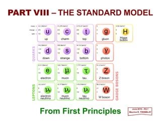
  • 7. According to the Standard Model of elementary particle physics, the universe is made of a set of fundamental spin-h/2 fermions, the leptons and quarks (see Table). The Particles 7 2017 MRT Quark Up u ⅔ 0.005 Down d −⅓ 0.01 Charm c ⅔ 1.5 Strange s −⅓ 0.2 Top (disc. 1994) t ⅔ 170 Bottom (disc. 1977) b −⅓ 4.7 Lepton Symbol Charge (e) Mass (GeV/c2)* Electron e− −1 0.000511 e-Neutrino νe 0 <7×10⁻⁹ Muon µ− −1 0.106 µ-Neutrino νµ 0 <0.0003 Tau τ− −1 1.7771 τ-Neutrino ντ 0 <0.03 * Masses given in units of 1Giga-eV/c2=1.782662×10−27 kg,with 1eV=1.602×10⁻¹⁹J and c is the velocity of light (in vacuum). Fermions interact through the exchange of spin-h bosons in a way that is precisely de- termined by local gauge invariance and through gravitation, and also through the ex- change of some spin-0 Higgs particles, which play a crucial role in generating mass.
  • 8. These fermions may be divided into three generations (or families) (see Table). 8 First Generation Second Generation Third Generation Leptons e−, νe µ−, νµ τ−, ντ Quarks u, d c, s t, b Each generation contains two flavors of Quark, which enjoy strong interactions, and two leptons, which do not. 2017 MRT Each particle has an associated antiparticle with the same mass but opposite quantum numbers, so there are antileptons like e+ (with L=−1) and antiquarks like d(with B=−⅓). The leptons carry unit lepton number L=+1, but zero baryon number, while the quarks have one-third (fractional)baryon number B=+⅓, but zero lepton number L=0. The net lepton number and net baryon number appear to be conserved in all the interactions, as of course is the net electric charge. The leptons group naturally into pairs because in all processes the total number of particles of each generation, for example: )()e()()e( eee νν NNNNL −−+≡ +− appears to be conserved (and similarly for (µ−,νµ) and (τ−,ντ)). These rules are often referred to as conservation of electron number Le, muon number Lµ, and tau number Lτ. The masses, me, mµ, and mτ, of the charged leptons e−, µ−, τ− exhibit no discernable pattern, so a fourth (or further generations) is considered to be unlikely. _
  • 9. Each of the quarks in the first Table can exist in three forms distinguished by the so- called color quantum number associated with the strong interaction coupling (i.e., an interaction is where the point particles or their constituents actually mix together via a potential – highlighted as in Figures) which can take the values red, blue, or green. 9 2017 MRT )]q()q([3 NNB −= There are no known interactions that mix quarks with leptons and hence the total quark number (i.e., the number of quarks minus the number of antiquarks, N(q)−N(q)) is conserved. This is referred to as the baryon number conservation since: This rule is crucial to the stability of protons and hence of matter itself. _
  • 10. In the Standard Model these fundamental particles undergo four known types of gauge interaction – gravitation, electromagnetism, and the weak and strong nuclear forces – and also interact with Higgs bosons. 10 rr mm GrV N 1 )( 21 ∝−= The Forces According to Newton’s nonrelativistic theory of gravitation, the potential energy between two point-particles of mass m1 and m2 that are separated by a distance r is: where GN is Newton’s gravitational constant (see Table). The potential acts only over r−1. Constant Symbol Value Newton’s gravitational constant GN 6.67259×10⁻¹¹ m3 kg−1 s−2 Velocity of light (vacuum) c 299,792,458 m s−1 Planck’s constant (Dirac’s h-bar) h≡h/2π 1.05457×10⁻³ J s Conversion constant hc 0.19733 GeV fm Fine structure constant α≡e2/4πεohc (137.03599)−1 Fermi constant GF/(hc)3 1.16637×10⁻⁵ GeV−2 2017 MRT A dimensionless measure of the strength of the gravitational coupling is given by GN m2/hc and if we insert a typical mass, such as that of the proton, mp, into the above equation we find that GN mp 2/hc≅10−40 is so extraordinarily small that gravity can safely be neglected in most practical aspects of particle physics.
  • 11. According to general relativity, gravity really couples to the total energy, E≡mc2, not just the rest mass, mo, and if we write GN m2/hc as GN E2/hc5 we find that the coupling is unity for E=EP ≡MP c2, where MP =√(hc/GN)=1.2×1019 GeV/c2, the so-called Planck mass. Hence, gravity certainly cannot be neglected if we want to explore what may happen at such very high energies, EP =pc (with the momentum p defined by de Broglie as p=h/λ= 2πh/λ where we can also identify D=λ/2π as lP at that energy scale), that is if we want to probe to distances of r≅lP, the Planck length, defined by lP=hc/EP=√(hGN /c3)=1.6×10−35 m. 11 Now, according to quantum field theory, the gravitational force is carried by the particle ‘quantum’ of gravitational radiation called the graviton, G (see Figure). Then GN m2/hc gives a measure of the probability of a graviton being exchanged, which is clearly very small unless energies approaching EP or distances approaching lP are encountered. 2017 MRT Since the gravitational force is of infinite range, these gravitons must be massless, and because in general relativity the quantum field represents fluctuations of the rank-2 metric tensor of space- time, gµν , it must be spin-2h. Technically, the fact that gravity is found to have a long range automatically means that the interaction energy depends on separation as 1/r. The graviton must have a mass mG=0 so that the force proportional to 1/r2 results from an interaction and its spin cannot be h/2 since their could be no interference between the amplitudes of the single exchange, and no exchange nor can it have spin-h because one consequence of spin-h is that likes repel, and unlike attract as is the case in electromagnetism. Spin-0 is also out of the question due to the gravitational behavior of the binding energies. The gravitational interaction of two masses, m1 and m2, represented (Left) classically by force of gravity and (Right) quantum mechanically by virtual graviton exchange (x-t plane). The factor κ =√(8πGN)/c2 is the gravitational coupling. 2m 1m 2m 1m G ct x κ ≅2×10⁶s⋅(kg⋅m)−½ κ
  • 12. Of more immediate concern is the electromagnetic interaction. According to Coulomb’s law, the interaction potential between particles with charges Q1 and Q2, respectively, separated by a distance r is: 12 The electromagnetic interaction between a positron e+ and an electron e−, represented (Left) classically by lines of force and (Right) quantum mechanically by virtual photon exchange with coupling strengths ±e. 2017 MRT Since all particle charges appear to be simple multiples of the electron’s charge (−e where e=1.60217×10⁻¹⁹ C (or A⋅s) since 1 C =1 A⋅s) a convenient dimensionless measure of the electro- magnetic coupling is α≡e2/4πεohc=e2/4π≅(137)−1≅0.007 if we adopt the Heaviside-Lorentz units (i.e., εo ≡1) and, as is common in particle physics, set h ≡c≡ 1. In these units, e= √(4πα)≅0.303 and is dimensionless. Note that the photon has no mass, mγ = 0. − e + e rr QQ rV 1 επ4 1 )( 21 o ∝= where εo is the permittivity of the vacuum, whose value depends on the units adopted for the charge. In MKS units, εo =8.854×10⁻¹² Fm−1 (A2 s4 m−3 kg−1) since 1 F=1 s4A2 m−2 kg−1. The quantum of the electromagnetic field is the photon, γ, and in quantum field theory it carries the electromagnetic force (see Figure). Since this force is also of infinite range, the photon must be massless, mγ = 0, and since it represents the U(1) gauge- invariant electromagnetic potential Aµ (a tensor of rank-1) it must have spin-h. It is this gauge-invariance property that ensures charge conservation and makes quantum electrodynamics (QED) a renormalizable theory (i.e., one that has only a finite number of divergences which, once subtracted away by absorption into the ‘bare’ parameters, leave a finite and sensible theory). − e + e γ +e ≅1.6×10⁻¹⁹ A⋅s −e
  • 13. The weak interaction, which cause β-decays (e.g., such as n→pe−νe or muon decay µ− →e−νeνµ), is of very short range. In fact, originally it was thought to be point-like (see Figure - Top Left) with a strength given by the Fermi (circa 1932) weak coupling constant GF (see previous Table). It is a universal interaction in the sense that all quarks and leptons have the same overall weak coupling strength. The dimensionless coupling for a particle having the typical hadronic mass mp is thus GF mp 2c4/(hc)3 ≅1×10⁻⁵ which, when compared to α≡e2/4πεohc≅7×10−3, explains why this is called the weak interaction. 13 (Top Left) The β-decay n → pe−νe by Fermi’s point-like interaction of strength GF. (Top Right) The same process mediated by virtual W− exchange, with coupling strength g. (Bottom) Another weak interaction process νµe− scattering mediated by virtual Z0 exchange. 2017 MRT According to the Glashow-Weinberg-Salam theory the weak force is in fact carried by very massive, spin-h, vector bosons W+, W−, and Z0 (see Figure) which generate an approximately SU(2) isospin-invariant weak interaction. The apparent weakness of the interaction is due, not to the smallness of the coupling 1×10⁻⁵ would seem to imply, but to the improbability of these very massive virtual particle being emitted. In fact, the weak interaction coupling g is comparable to e above, with GF ~ g2/MW 2 ~ e2/MW 2. More precisely, the couplings are related by: where sin2θw =0.222±0.011(1994),θw being the Weinberg weak mixing angle between the electromagnetic and weak interactions. Given our knowledge of α, GF , and sin2θw , our equation above can be used to deduce that MW ≅80 GeV/c2 and hence that the range of the weak interaction is ~ h/MWc ≅ 2.5×10⁻¹⁸ m ≅0.003 fm (with 1 fm =10−15 m). − e n p FG eν − e n p eν W− g g Z0 g g − e− e µν µν w F cMcM g c G θ α 242 W 2 W 2 3 sin2 π 24)( == hh ⇒ _ _ _
  • 14. Parity is not conserved in weak interactions because these W bosons couple only to left-handed (L) chiral projections of the quark and lepton fields. This means that the Ws couple to relativistic particles (i.e., with E>>mc2) only if they are spinning left-handedly about their direction of motion (see Figure). The SU(2)L isospin symmetric weak coupling of left-handed fermions is often called quantum flavor dynamics (QFD). 14 Particles traveling along an arbitrary positive z-direction with (Left) left-handed (anticlockwise) or (Right) right-handed (clockwise) spins along their directions of motion. Try it with your left / right hands. The particles’ spin is represented by the hashed arrow ( ⋅⋅⋅⋅ for tip and ×××× for base). 2017 MRT It turns out that if we start with a renormalizable SU(2) invariant gauge theory, which necessarily has massive W and Z fields, but then spontaneously break the symmetry by adding a Higgs scalar boson that has nonvanishing vacuum expectation value, W and Z (and in fact that quarks and leptons too) acquire finite masses, yet the renormalizability is retained. As a result of mixing with the proton (with mixing angle θw) the Higgs boson is not predicted, but is expected to be of the same order as MW. A chiral phenomenon is one that is not identical to its mirror image. The spin of a particle may be used to define a handedness, or helicity, for that particle which, in the case of a massless particle, is the same as chirality. A symmetry transformation between the two is called parity. Invariance under parity by a Dirac fermion is called chiral symmetry. An experiment on the weak decay of Cobalt-60 (i.e., 60Co) nuclei carried out by Chien-Shiung Wu and collaborators in 1957 demonstrated that parity is not a symmetry of the universe. The helicity of a particle is right-handed if the direction of its spin is the same as the direction of its motion (see Figure). L.H. Nature has favored ×××× ⋅⋅⋅⋅ z R.H. ×××× ×××× z
  • 15. Finally, we come to the strong force that binds quarks together to form hadrons, and hadrons into complex nuclei. This force is associated with the color coupling, which can take one of three possible values: red (R), green (G) or blue (B). The strong force is invariant under transformations among these three colors. Indeed, the nature of the strong force can be deduced simply by demanding that it should obey an exact local SU(3)C color symmetry (i.e., the C subscript), analogous to the U(1) invariance of electromagnetism. The massless quanta of this quantum chromodynamics (QCD) color field are called gluons, g (e.g., see Figure - Left), and because of the SU(3)C invariance it turns out that there must be 32 −1=8 different color combinations of gluons. And since the gluons carry color they can also couple to each other (e.g., see Figure - Right). 15 (Left) A quark-antiquark interaction by virtual gluon exchange, with strong coupling strength gs. (Right) The coupling of two gluons by gluon exchange, also of strength gs. 2017 MRT g qq q q gs gs g g g g g gs gs The strength of the strong coupling, gs, gives the probability of a quark or gluon emitting a gluon as in the Figure, and it is convenient to introduce: π4 2 s s g ≡α
  • 16. Before we can comment on the magnitude of the αs coupling, we have to take note of the fact that ‘vacuum polarization’ (i.e., the creation of virtual particle-antiparticle pairs) greatly complicates the description of relativistic quantum states. The uncertainty principle permits the existence of such pairs of particles (e.g., the best known being the positron e+ and electron e− pairs), each of mass me, for time periods T less than h/2mec2 (see Figure). 16 Virtual e+e− creation in the electromagnetic photon field, with coupling strength √α = e/√(4πεohc). 2017 MRTα α − e + e If the coupling that determines the probability of such pair creation is small (e.g., like the fine structure constant, α =e2/4πεohc, in QED), this effect can be treated as a small perturbation. This is the basis of perturbative quantum field theory, in which physical quantities are represented as power series in α. It successfully accounts for such quantities as the anomalous magnetic moments of the electron and muon, and the Lamb shift in atoms, for example, which are a direct result of vacuum polarization.
  • 17. Because of this vacuum polarization screening effect, the electromagnetic coupling varies with distance, r (see Figure), so that the fine structure constant α is not really a constant at all but varies with r. It turns out that the e+e− loop gives: 17 A negative charge, represented by a ‘point’ particle, which is ‘screened’ by vacuum polarization (i.e., the creation of e+e− pairs) [how organized the spread of polarization is is a matter of speculation] making the whole QED-picture-view of an electron as ‘fuzzy’. 2017 MRT In QCD it is found that similarly (i.e., for r>>hc/ΛC): 1 o ln π2 )( −                 Λ ≅ r cb r C s h α 1 e 1ln π3 1)( −                 +−≅ crm r hα αα where α is the value measured at large r (i.e., r>>h/mec, the electron’s Compton wavelength). Evidently, α is predicted to become very large at very short distances (i.e., as r→h/[mecexp(3π/α)]≅10−300 m), by which point perturbation theory must break down. Our equation above still indicates that QED alone cannot be correct at high energies! where bo is a constant (see Renormalization chapter), is positive because the self-coupling of the gluons results in antiscreening. Hence αs →0 as r→0, which gives rise to the so-called asymp- totic freedom (i.e., the fact that quarks and gluons inside a hadron behave like free particles when very close together). On the other hand, αs apparently diverges as r→RC ≡hc/ΛC, where ΛC is the hadronic energy scale. This divergence simply heralds the breakdown of perturbation theory, of course, but nonetheless it leads us to expect that the strength of the force between quarks will increase if they are pulled apart. As a result, quarks and gluons are confined inside hadrons which size is of order RC. + − + − + − + − + − + −+− −−−− + − + − + −
  • 18. The crucial parameter characterizing the strong interaction is the hadronic energy scale ΛC. It turns out to be: 18 2017 MRT GeV3.02.0 −≅ΛC Not surprisingly, it is of the same order of magnitude as the masses of the lightest hadrons. In summary, in order to account for all the known types of interactions, we need the spin-2h graviton and the 12 spin-h gauge bosons listed in the Table. The Standard Model of particle physics is thus gravitation, together with the above SU(3)C⊗SU(2)L⊗U(1)Y gauge-invariant strong and electroweak interactions. After the spontaneous breaking of the symmetry as a result of the Higgs coupling, we are left with SU(2)L⊗U(1)EM as exact gauge symmetries, and the 8 gluons g1…g8 and the photon γ as massless particles. Constant Symbol Spin (h) Mass (GeV/c2) Charge (e) Graviton† G 2 0 0 Photon γ 1 0 0 Charged weak bosons W± 1 81.5 ±1 Neutral weak boson Z0 1 92.5 0 Gluons* g1…g8 1 0 0 Higgs H 0 126 0 * <0.0002 eV/c2 (Experimental limit). †If I were to speculate based on a discernable pattern, since the Higgs generates the mass of both weak bosons would it be conceivable that the photon and the gluons generate the graviton in some theoretically yet-to-be-formulated model? TBD…
  • 19. As we have just seen, the strength of the color coupling, αs, is not constant but becomes stronger as the separation between the quarks increases (i.e., αs(r)≅1/[(bo/2π) ⋅ln(hc/ΛC r)]). So, unlike electrons in atoms, quarks are permanently bound together, and confined within hadrons. It is only color-neutral combinations of quarks that can have a vanishing color coupling and hence occur as free particles. There are two different ways in which these colorless hadrons can be made, given the three different colors of quarks qk (k = R for red,G for green, andB for blue): 19 2017 MRT ∑=+−= kji kji kji 321 B 3 R 2 G 1 B 3 G 2 R 1 qqq 6 1 )qqqqqq( 6 1 B εK The Hadrons where εijk is the anti-symmetric permutation tensor, or; ∑=++= k kk 21 B 2 B 1 G 2 G 1 R 2 R 1 qq 3 1 )qqqqqq( 3 1 M These hadrons are color-neutral in a somewhat analogous way to that whereby one can produce white either by an equal mixture of the three primary colors (red, green, and blue) like B above, or by mixing green (say) with its complementary color, magenta (=red+blue), like M above. 2) We can take a quark q1 of one color and an antiquark q2 which has the opposite (complementary) color, and thereby make a meson: 1) We can take an admixture of three quarks, q1, q2, and q3, say, which have different colors, and thereby obtain a baryon: _
  • 20. The lightest baryons (B=1) and mesons (B=0) are listed in the following Table. 20 2017 MRT Baryons Spin-h/2 Spin-3h/2 Quark Content Particle Mass (GeV/c2) Particle Mass (GeV/c2) uuu ∆++ 1.232 uud p 0.9383 ∆+ 1.232 udd n 0.9396 ∆0 1.232 ddd ∆− 1.232 uus Σ+ 1.1894 Σ+ (1385) 1.3828 uds Σ0 1.1925 Σ0 (1385) 1.3837 Λ(*) 1.1156 dds Σ− 1.1973 Σ− (1385) 1.3872 uss Ξ0 1.3149 Ξ0 (1530) 1.5318 dss Ξ− 1.3213 Ξ− (1530) 1.5350 sss Ω− 1.6724 Mesons Spin-0 Spin-h Quark Content Particle Mass (GeV/c2) Particle Mass (GeV/c2) ud, du π± 0.13957 ρ± 0.770 (uu –dd)/√2 π0 0.13497 ρ0 0.770 us, su K± 0.49365 K*± 0.8921 ds,sd K0,K0 0.49767 K*0, K*0 0.8921 (uu –dd)/√2 η 0.5488 ω 0.782 ss η′ 0.9575 φ 1.0194 cd,dc D± 1.8693 D*± 2.0101 cu, uc D0,D0 1.8645 D*0, D*0 2.0072 cs,sc Ds ± 1.969 Ds*± 2.113 cc ηc 2.980 ψ 3.0969 ub, bu B± 5.278 B*± 5.325 db,bd B0,B0 5.279 B*0, B*0 5.325 sb,bs Bs 0,Bs 0 5.366 Bs*0, Bs*0 5.415 bb ηb 9.388 ϒ 9.4603       * Heavier baryons, such as Λc = udc, can be made by substituting the heavier c, b, or t quarks for any of those shown.
  • 21. Baryons such as the proton p=uud and neutron n=udd come in states where the 3 quark composing them have their spins oriented ↑↑↓ (i.e., up-up-down) so that the pro- ton and neutron both have spin-h/2. For other particles, the spins can be ↑↑↑ and so there are heavier spin-3h/2 states made of the same set of quarks (i.e., ∆+ and ∆0, respecti-vely) that are unstable and decay (e.g., ∆+ →pπ0, where π0 is a neutral pion). Mesons with B=0 consist of a quark (B=⅓) together with an antiquark (B=−⅓) (e.g., the spin-0 π+=ud is an ↑↓ spin state, while the spin-h ρ+ is made of the same quarks but in the ↑↑ spin state). 21 2017 MRT 2 c mm CΛ +≈ currenttconstituen Since quarks are always confined within hadrons, it is not possible to measure their masses directly. The values quoted in the previous Table are so-called current quark masses deduced from what is called current algebra. It is important to notice that the light hadrons (i.e., those made of only u, d, and s quarks) are very different from most of the composite states found in physics because their masses are much lighter than the sum of the individual current algebra quark masses. The mass of a hadron can be thought of as being made up of the sum of the kinetic energies of the quarks, which are of order ΛC (i.e., the hadronic energy scale), together with their current (algebra) masses. It is sometimes useful to introduce a constituent quark mass of magnitude: _ so that, in terms of constituent masses, mp ≅2mu +md for example. Although the current masses of the u and d are slightly different, their constituent masses are almost identical (both ~ΛC /c2), which is why the proton and neutron masses are almost equal, mp ≅mn.
  • 22. The resulting symmetry under the interchange of u and d quarks produces the SU(2) isospin symmetry of nuclear physics. The s quark is not all that much heavier, so there is also an approximate SU(3) flavor symmetry among those hadrons that can be made out of just u, d, and s quarks. The c, b, and t quarks are much heavier than ΛC, however, so there is not much difference between their current (algebra) and constituent masses. 22 Because the heavier quarks undergo weak decays (e.g., s→ue−νe, c→sµ+νµ, b→cud, &c.), the proton is the only stable baryon. The neutron is nearly stable, with a lifetime τ ~ 15 minutes for its decay, n→pe−νe (i.e., in terms of quarks, d→ue−νe), because mn ≅mp, and of course it is stable when inside a nucleus if its extra binding energy exceeds (mn −mp −me)c2. In these decays the total number of quarks, and hence the baryon number B, is conserved. Indeed, B is conserved in all interactions, a fact that is crucial to the stability of atomic matter. Quark diagrams for the dominant decays of the lightest mesons, π+ and π0. 2017 MRT All of the mesons are unstable because even the lightest, the pion, can decay, viz: as a result of quark-antiquark annihilation (see Figure). γγπµπµπ 0 µµ →→→ −−++ and, νν + π µν + µu d W+ )d(u 0 π )d(u γ γ _ _ __
  • 23. Any attempt to knock a quark out of a hadron, for example by hitting it with an electron (see Figure - Left), or spontaneous hadronic decay processes (see Figure - Right), involve a stretching of the color lines of force. This results in the creation of quark- antiquark qq pairs in the vacuum, so the lines of force get shortened, but they still always begin on a q and end on a q. Hence, a quark that is knocked out of one hadron necessarily ends up inside another. The forces between quarks and gluons increase with distance, so they are confined within hadrons whose radii: 23 (Left) Deep inelastic electron-proton scattering in which a quark is knocked out of the proton by a virtual photon γ. This is followed by the creation of qq pairs in the stretched color field and hence the production of hadrons. (Right) The decay of the unstable ρ+ meson into a π+π0 state through dd creation. C C c RR Λ ≡≈ h 2017 MRT and typically about 10−15 m (1 fm), because the strong color interaction energy scale is approximately ΛC ~ 0.2-0.3 GeV. e p q q q N e γ d d d u u d + ρ 0 π + π g g _ _ _ _
  • 24. Of course, even though hadrons are color-neutral they can still interact with each other by the exchange of gluons and quarks (see Figure - proton-proton scattering with p=uud). The force results from the polarization of the color charge. 24 2017 MRT Proton-proton scattering by (Left) gluon exchange, (Middle Left) quark exchange, (Middle Right) π0 pion exchange (i.e., as a result of the bonding of the exchanged quarks in Middle Left), and (Right) ‘Pomeron’ exchange (i.e., interacting gluons). If quarks are exchanged over distances >RC, they may bind together to form mesons (see Figure - Middle Right) which is why the long-range part of the interaction was originally identified by Yukawa as meson exchange. The gluonic force may similarly be identified with the ‘Pomeron’ effect (i.e., interacting gluons), which was introduced in the late 1950s to account for elastic and diffractive scattering processes in which there is no exchange of flavor quantum numbers. Gluons carry color and hence couple to each other (see Figure - Right), whereas photons of course do not carry charge and so cannot couple together directly. g g 0 πq p p p p ‘Pomeron’ exchange
  • 25. In particles made of heavy quarks (i.e., mqc2 >>ΛC), such as the ψ(cc) charmonium states, the ϒ(bb) bottomonium states (N.B., the high mass of the top quark, toponium tt, does not exist since the top quark decays through the electroweak interaction before a bound state can form), the velocities of the quarks are very much less than the speed of light, c, and relativistic effects should not be too important. In such cases it is reasonably satisfactory to treat the particles as if they were made of just their constituent valence quarks, with an interaction potential between the q and q that takes the form: 25 2017 MRT r r rV s )( 3 4 )( α −= where the factor of 4/3 comes from the sum over all possible colors of quarks, and over the colors of the gluons that can be exchanged. Since αs varies with r in αs(r)≅1/[(bo/2π)ln(hc/ΛC r)], this can be rewritten:       Λ −≈ r c rb rV C h ln π2 3 4 )( o or, to represent better the behavior at large r (i.e., where αs(r) ≅1/[(bo/2π)ln(hc/ΛC r)] is invalid): rT r rV s o 3 4 )( +−≈ α where To is called the ‘string tension’. _ _ _ _
  • 26. This arises because gluons interact with each other and so produce a cigar- or string- shaped distribution of color lines of force (see Figure), quite different from Coulomb’s law. Since the energy density in the ‘string’ is approximately constant, the energy of the string increases with r and gives rise to a potential V(r)~To r at large r. It therefore needs an infinite amount of energy to drag the quarks apart (unless new qq pairs are created), which is presumably the explanation for the confinement of quarks in hadrons. 26 The long-ranged interaction in QED, in which the field’s energy density represen- ted by the separation of the lines of force ~r−2, contrasted with the QCD interaction of a quark and an antiquark, in which the energy density is constant inside the color ‘cigar’ or ‘string’. 2017 MRT − e + e r QED QCD q q _
  • 27. Another important reason for this confidence in QCD, and indeed in the whole SU(3)⊗SU(2)⊗U(1) Standard Model of the strong, weak, and electromagnetic properties of matter, is that it correctly predicts the outcome of a great variety of scattering experiments: electron-positron scattering (e.g., e+e−), deep inelastic scattering (e.g., e−p), and hadron scattering (e.g., pp), to name a few. 27 In a two-body scattering process such as (see Figure - Left): dcba +→+ Scattering According to quantum theory a high-energy beam of energy E=p/c has an associated wavelength λ=hc/E (i.e., λ∝1/E), which determines the shortest distance which can be resolved. Hence, to probe short distances we require very high energies. each particle has four-vector momentum matrix: T ][ pcEp =µ where µ =0,1,2,3 corresponding to the timelike, 0, and the three spacelike components, 1,2,3, respectively, E being its energy and p its momentum, in a given Lorentz frame. We will employ the usual Minkowski space-time metric, ηµν , with sig- nature (+,−,−,−), so that the Lorentz-invariant scalar product: 2 o 2 23 0 2 )()( cm c E ppppppp =−      =≡≡⋅≡ ∑∑= p µν ν µν µ µ µ µ η where mo is the is the particle’s rest mass (moc being the reference or standard momentum kµ ). It is usually more convenient to work in units where c≡ 1 so this mass-shell condition above becomes p2 =m2 with mo≡m from now on. _ (Left) The scattering process a +b→ c +d with the four-momenta labelled. (Right) This same process in the center-of-mass (CM) system. Here θ is the scattering angle of particle c with respect to the beam direction and d Ω is the element of solid angle into which c is scattered. 2017 MRT
  • 28. The scattering process can be described by three Lorentz-invariant Mandelstam variables: 28 2017 MRT 22 22 22 )()( )()( )()( bcda bdca dcba ppppu ppppt pppps −=−≡ −=−≡ +=+≡ which can readily be shown to satisfy: 2222 dcba mmmmuts +++=++ so only two of the s, t, or u are independent. ],[],[ pp −== bbaa EpEp and represents the square of the total center-of-mass energy, ECM ≡Ea +Eb, while the center- of-mass frame scattering angle θ is given by: θcos222 2222 cacacacaca EEmmppmmt pp+−+=⋅−+= At high energies, where all the masses are negligible, so that |pa|~Ea, &c., we find: )cos1( 2 )cos1( 2 θθ +−≈−−≈ s u s t and In the center-of-mass system of the scattering process (see previous Figure - Right): 22 ],[ CMEEEs ba =+= 0 and:
  • 29. The differential cross section, dσ, which is the probability per unit incident flux of particle c being scattered into a given element of solid angle dΩCM =dϕ d(cosθ) (see previous Figure - Right), is given by: 29 2017 MRT 2 2 π64 M a c sd d p p = ΩCM σ or from t~2|pa||pc|cosθ above (N.B., s=ECM 2=(Ea +Eb)2): ∫ Ω=+→Γ d m cba a 2 22 π32 )( M p 2 2 2 2 6π1 11 π64 1 MM sstd d a ≈= p σ Similarly, the width for the decay a→b+c is: where p is the momentum of particle b or c in the rest frame of a and the integration is over all directions of p. 2 2 π64 1 M sd d ≈ ΩCM σ where M is the scattering amplitude. We have to integrate this over the scattering angle θ to get the actual scattering cross-section, σ = ∫(dσ /dΩCM)dΩCM =∫(dσ /dΩCM)sinθdθdϕ. Now, if we neglect the masses:
  • 30. In classical mechanics, the equations of motion of a dynamical system can be derived from the Lagrangian function L(qi,qi) (N.B., the dot ‘⋅⋅⋅⋅’ over the generalized coordinate q is shorthand for q=∂q/∂t) with qi being the generalized coordinates of the system, which is defined to be: 30 2017 MRT )()(),( iiii qVqTqqL −= && Field Equations ⋅⋅⋅⋅ where T is the kinetic energy and V is the potential energy. The action S involved in the motion of the system from one configuration at time t1 to another at t2 is given by: ∫= 2 1 t t tdLS and, according to the principle of least action, the path actually taken by the system will be the one that minimizes S. It is readily shown that the condition for S to be a minimum is that L should obey the Euler-Lagrange equations: 0= ∂ ∂ −        ∂ ∂ ii q L q L td d & These equations of motion are equivalent to Newton’s laws of motion. Thus, for a qi →xi = x example, by using T=½mx2 in L(x,x)=T(x)−V(x) above one can deduce from the Euler- Lagrange equations that a particle’smotion will obeyNewton’s second law if expressed as: where F(x) is the force at point x. ⋅⋅⋅⋅ )()(2 2 xFx x ≡−= V td d m ∇∇∇∇ ⋅⋅⋅⋅ ⋅⋅⋅⋅ ⋅⋅⋅⋅
  • 31. For the purpose of keeping the relativistic covariance of the physics more apparent, it is convenient to replace L by the Lagrangian density function L so that: 31 2017 MRT ∫= x3 dL L and thus the action S above can also be rewritten covariantly as: ∫∫∫ === xddtdtdLS 43 LL x since d4x=dtd3x where x is the space-time four-vector with components xµ =[t,x]. In relativistic field theory, we replace qi by the field φ(xµ), so the index i is replaced by the space-time coordinates x≡xµ, and the Lagrangian is a Lorentz scalar function of φ(x). Since each ∂/∂x can be associated with a similar term involving ∇∇∇∇, we can make up the covariant derivative (and its equivalent shorthand notation): 0 )()()( 3 0 3 1 = ∂ ∂ −         ∂∂ ∂ ∂= ∂ ∂ −         ∂∂ ∂ ∂ ∂ +         ∂∂ ∂ ∂ ∂ ∑∑ == φφφφφ µ µ µ LLLLL i i i t xt So, for a given choice of Lagrangian L(φ,∂µφ), this set of space-time Euler-Lagrange equations can be used to deduce the equations that will be satisfied by the field φ(x). and so the Euler-Lagrange equations become: φ φ µµ ∂≡ ∂ ∂ x
  • 32. Thus, for a free scalar (i.e.,spin-0) particle of (rest) mass m the Lagrangian density is: 32 2017 MRT 22 2 1 ))(( 2 1 φφφ µ µ µ m−∂∂= ∑L and so the differentials are: φφ φφ φφφ φφ µ µ µ µ µµ 222 2 1 0)(0))(( 2 1 )()( mm −=      ∂ ∂ −= ∂ ∂ ∂=−      ∂∂ ∂∂ ∂ = ∂∂ ∂ ∑ LL and which, when substituted into the space-time Euler-Lagrange equations, gives the Klein- Gordon equation: 0)][( )( 222 =+=+         ∂∂=+∂∂= ∂ ∂ −         ∂∂ ∂ ∂ ∑∑∑ φφφφφφ φφ µ µ µ µ µ µ µ µ µ mmm LL where we have introduced the d’Alembertian operator: 2 2 2 ∇− ∂ ∂ =∂∂= ∑ tµ µ µ In view of the usual quantum-mechanical operator replacements (h≡1) E→i∂/∂t and p→ −i∇∇∇∇ which, in four-vector notation, given [E,p]→[i∂/∂t,−i∇∇∇∇]=i[∂/∂t,−∇∇∇∇], gives the four- momentum as: µµ ∂−→ ip Now, φ +m2φ =0 simply ensures that the field obeys the mass-shell condition p2=m2.
  • 33. The flow of particles is represented in space-time by the current four-vector: 33 2017 MRT *)*( φφφφ µµµ ∂−∂= iJ ],[ Jρµ =J where ρ is the particle density and J is the flux current. It is a conserved quantity: 0=∂=•+ ∂ ∂ ∑µ µ µ ρ J t J∇∇∇∇ For example, the current for the scalar boson field φ is: In order to discuss vector (i.e., spin-h) particles, we need to consider properties of the classical electromagnetic field, which are summarized in Maxwell’s equations: 0 B EB J E BE = ∂ ∂ =• = ∂ ∂ =• t t ++++××××∇∇∇∇∇∇∇∇ −−−−××××∇∇∇∇∇∇∇∇ and ,, 0 ρ where E and B are the electric and magnetic field strengths, respectively. Here ρ is the charge density and J is the charge-current density (which, unlike Jµ =[ρ,J] includes a factor of e). As usual in particle physics, we use the Heaviside-Lorentz units where εo ≡1.
  • 34. It is convenient to introduce the four-vector potential: 34 2017 MRT µννµµν AAF ∂−∂= ],[ Aφµ =A so that: φ∇∇∇∇−−−−××××∇∇∇∇ t∂ ∂ −== A EAB and Then, since ∇∇∇∇•∇∇∇∇××××A=0 and ∇∇∇∇××××∇∇∇∇φ =0, the last two Maxwell equations (i.e., ∇∇∇∇•B=0 and ∇∇∇∇××××E++++∂B/∂t=0) are satisfied automatically, while the first two (i.e., ∇∇∇∇•E=ρ and ∇∇∇∇××××B−−−− ∂E/∂t=J) can be re-expressed in terms of the field-strength tensor: in the form: νµ µ µ νν µ µν µ JAAF =         ∂∂−=∂ ∑∑ where Jµ =[ρ,J] is the charge-current four-vector that satisfies Σµ∂µ Jµ =0.
  • 35. The Maxwell equations can be derived from the Lagrangian (density): 35 2017 MRT χχ φφ χ µµµ ∂+→     ∂ ∂ +→ → AA t ∇∇∇∇−−−−AA ∑∑ −−= µ µ µ µν µν µν AJFF 4 1 L By substituting this Lagrangian into the space-time Euler-Lagrange equations and minimizing the action with respect to each component Aµ, we again obtain Σµ ∂µ Fµν =Jν. In quantum field theory, Aµ can be regarded as the wave function of the photon, and the expression Σµ ∂µ Fµν =Jν is then the wave equation that the photon has to satisfy. However, the B=∇∇∇∇××××A and E=−∂A/∂t−−−−∇∇∇∇φ equations do not specify Aµ uniquely in terms of the physical E and B fields, since under a so-called ‘gauge’ transformation of the form: where χ can be any scalar function of the space-time coordinate x, the fields B, E, and hence Fµν are all completely unchanged, as may readily be checked by direct substitu- tion in B=∇∇∇∇××××A, E=−∂A/∂t−−−−∇∇∇∇φ, and Fµν =∂µ Aν −∂ν Aµ (Exercise). It is often useful to make use of this gauge freedom and fix the gauge so that Aµ satisfies the Lorentz condition: in which case Σµ ∂µ Fµν = Aν −∂ν (Σµ ∂µ Aµ)= Jν reduces to Aµ =Jµ. Redundancy! 0=∂∑µ µ µ A
  • 36. For non-interacting photons, Jµ =0, and Aµ =Jµ is simply the requirement that the mass-shell condition p2 =m2=0 be satisfied (i.e., we will use the conventional q2 =0 for a massless photon of four-momentum q). The plane-wave solutions have the form: 36 2017 MRT xqi qA ⋅− = e)(µµ ε with q2 =0, where ε µ is the polarization vector of the photon (N.B., we now use the four- vector shorthand q⋅x ≡Σµ qµ xµ). The Lorentz condition Σµ ∂µ Aµ=0 requires that: 0=∑µ µ µεq which reduces the apparent four degrees of freedom to three. However, one of these three is spurious (i.e., a dummy one) because the Lorentz condition does not completely fix the gauge. Transformations like Aµ→Aµ +∂µχ are still allowed provided χ =0; for example χ=iaexp(−iq⋅x). On substituting this, together with Aµ=ε µ(q)exp(−iq⋅x), into Aµ →Aµ +∂µ χ one sees that no physical quantity is changed by the replacement εµ→εµ +aqµ so two polarization vectors that differ by some multiple of the four-momentum describe the same photon. We may use this freedom to set ε0≡0, whereupon the Lorentz condi- tion Σµ ∂µ Aµ=0 becomes q•εεεε=0 and the photon has only transverse polarization. This (non-covariant) choice of gauge is known as the Coulomb gauge. For a photon travelling along the z-axis, the two independent polarization vectors can be taken to be εεεεR,L = m(1/√2)(êx ± iêy) where êk are unit vectors along the k-axis (k=1,2,3). These describe a photon with spin projection along the direction of motion (i.e., helicities) of ±1, respec- tively (as can be easily verified from their behavior under rotations about the z-axis).
  • 37. For a free spin-h particle of (rest) mass M, we take: 37 2017 MRT instead of L =−¼Σµν Fµν Fµν−Σµ Jµ Aµ above with Jµ =0. This leads, using the space-time Euler-Lagrange equations again, to the Proca equation: ∑∑ +−= µ µ µ µν µν µν AAMFF 2 2 1 4 1 L 02 =+∂∑ ν µ µν µ AMF If we take the divergence of this equation (i.e., operate on it with ∂ν), we find Σν ∂ν Aν =0 (for M2 ≠0). This is not a necessary condition (i.e., not a choice of gauge). The Proca equation then becomes: 0)( 2 =+ ν AM which leads again to the mass-shell condition p2 =M2≠0. Polarization vectors of a massive spin-h particle automatically satisfy Σµ qµε µ =0, but as there is no gauge invariance there are three degrees of freedom, corresponding to helicities ±1 and 0. For example, a particle with momentum q along the z-axis has ε (r=±1) =m(1/√2)[0,1,±i,0] and ε (r=0)=(1/M)[|q|,0,0,E]. They satisfy the completeness relation: 2 )()( *][ M qq r rr νµ µννµ ηεε +−=∑ Ok,from now on we set h≡1 so as to describe spin-h particles will be spin-1 particles.
  • 38. We now turn to spin-½ particles (with h≡1) which obey Fermi-Dirac statistics (N.B., as opposed to spin-0, spin-1, and spin-2 particles which obey Bose-Einstein statistics), for which the situation is more complicated. Fermions are described by four-component spinor fields: 38 2017 MRT             = 4 3 2 1 ψ ψ ψ ψ ψ Fermions For free particles of (rest) mass m (with h≡1), the spinor ψ (x) satisfies the Dirac equation: 00o =         −∂⇔=         −∂ ∑∑ ψγψγ µ µ µ µ µ µ micmi h where the γ µ are a set of 4×4 matrices. A more compact Feynman slash notation, in which: is often used. With this notation, the Dirac equation above becomes (Dirac 1928): 0)( =−∂/ ψmi aa /≡∑µ µ µ γ
  • 39. In order that the equation obtained by operating with (iΣµγ µ∂µ +m) on (iΣµγ µ∂µ −m)ψ =0 should be the Klein-GordonequationΣµ∂µ ∂µφ +m2φ =0(so as to guarantee that E2 =p2 +m2), we require (i.e., the Clifford algebra): 39 2017 MRT µνµννµνµ ηγγγγγγ 2},{ =+≡ called an anticommutator (to contrast with the commutator [σµ,σ ν ]≡σµσν −σνσµ). All of the spin properties of the theory follow from this equation for the γ matrices and particular representations are not necessary. However, it is often much easier to work with a suitable chosen representation. We shall take the γ matrices to be unitary, so from the anticommutator {γ µ,γν} above we find (Exercise): kk γγγγ −== †0†0 and These equations can be summarized by the relation: 00† γγγγ µ k = The ‘standard’ (or Pauli-Dirac) representation is given by:       − =      = 0 0 0 00 k kk I I σ σ γγ and where I is the 2×2 unit matrix and the σ k are the usual 2×2 Pauli matrices:       − =      − =      = 10 01 0 0 01 10 321 σσσ and, i i
  • 40. It is convenient to define a fifth matrix, usually denoted by γ 5, as: 40 2017 MRT 32105 γγγγγ i≡ Clearly from {γ µ,γ ν}: 50123†0†1†2†3†5 γγγγγγγγγγ ==−= ii We also find that (Exercise): 0},{1)( 525 == µ γγγ and In our standard representation:       = 0 05 I I γ and (Exercise): kk γγγγ −== †0†0 and
  • 41. 41 2017 MRT 0=−∂− ∑ ψγψ µ µ µ mi The Hermitian conjugate of the Dirac equation iΣµγ µ∂µψ −mψ =0 is: 0††† =−∂− ∑ ψγψ µ µ µ mi which, on multiplying by γ 0 from the right: 00†0†† =−∂− ∑ γψγγψ µ µ µ mi and using γ µ† =γ 0γ µγ 0 and the fact that (γ 0)2 =1, becomes: where we have introduced the adjoint (row) spinor: 0† γψψ ≡ On multiplying iΣµγ µ∂µψ −mψ =0 from the left by ψ and −iΣµ ∂µψγ µ −mψ =0 from the right by ψ and subtracting, we deduce that: ψγψ µµ ≡J is the probability flux or current that satisfies the conservation equation Σµ∂µ Jµ =0. The probability density: is positive definite. This was part of the original motivation for the introduction of Dirac’s equation (as the story goes, he was staring into a fireplace at Cambridge). ψψψγψρ †00 ==≡ J _ _ _
  • 42. Bilinear quantities with simple Lorentz transformation properties can be built from ψ and ψ . It can be shown (Exercise) that: 42 2017 MRT ψψ ψγγψ ψγψ ψγψ ψψ µν µ µ Σ 5 5 transform as a scalar, pseudoscalar, vector, axial-vector and (antisymmetric) tensor, respectively, where the tensor is the commutator of the γ µ (i.e., that set of 4×4 matrices): ],[ 2 )( 2 νµµννµµν γγγγγγ ii ≡−≡Σ The Lagrangian which, using the space-time Euler-Lagrange equations, leads to the free Dirac equation (iΣµγ µ∂µ −m)ψ =0 is: ψψψψ mi −∂/=L or, using the Feynman slash notation (i.e., a≡Σµγ µaµ): ψψψγψ µ µ µ mi −∂= ∑L _
  • 43. We must next consider the coupling between spin-½ and spin-1 particles. 43 2017 MRT 10† − −== Cψcc T γψψ 0)( =−−∂∑ ψψγ µ µµ µ mAei The corresponding equation written for an antiparticle (i.e., with e→−e) is satisfied by: *0ψγψψ TT CCc =≡ with ψ =ψ †γ 0 and where c, the notation for a charge-conjugation matrix, satisfies: T µµ γγ −=− CC 1 So, if ψ is regarded as a field operator that annihilates a particle or creates an antiparticle, then ψ c is the charge-conjugation field, which annihilates an antiparticle or creates a particle. From ψ c=Cψ T= Cγ 0 Tψ * above we find that: In classical electromagnetism, the force experienced by a particle of charge e in an electromagnetic field is the Lorentz force F=e(E++++v××××B), which is obtained if in the classical Lagrangian we make the replacement pµ →pµ−eAµ, where Aµ is the vector potential. Similarly, in quantum theory we make the replacement i∂µ →i∂µ −eAµ. Hence, the Dirac equation for a particle in an electromagnetic field is: _ _
  • 44. Some useful bilinear identities that follow from these results are: 44 2017 MRT             − − == 0 0 01 10 01 10 02 γγiC 12212 1 121 )()( ψψηψηψψψψψ Γ=Γ−=Γ−=Γ − TTTTT CCcc where by using C −1γµ C=−γµ T we find that η=(1,1,−1,1,−1) for Γ={1,γ 5,γ µ,γ µγ 5,Σµν}, respectively (N.B., in transposing, add a ‘−’ sign since fermion fields anticommute). One consequence of the above results is that the current J µ=ψ γ µψ satisfies ψγµψ =−ψ cγµψ c while ψ cψ c =ψγµψ , which is just what one would expect to be the result of the charge- conjugation operation. In the standard representation (N.B., differs from PART IV’s Dirac basis) of γ 0 and γ k : More generally, in all representations of interest, we have: CCCC −=== −1†T             − − =             − − =             =             = 0 0 0 0 0 0 0 0 10 01 10 01 0 0 0 0 01 10 01 10 10 01 10 01 3210 γγγγ and,, i i i i a possible choice for C that satisfies C−1γµ C=−γµ T is: _ _ _ _ _
  • 45. We shall later meet two important special types of fermion field. The first is the chiral or Weyl fermion defined by: 45 2017 MRT RLRL ,, 5 ψψγ m= where the suffixes L, R are used to indicate that these eigenstates of γ 5 correspond to left-, right-handed chiralities (i.e., which in the zero-mass or infinite-momentum limit correspond to helicities m½), respectively. We can project out the left- or right-handed parts of a general spinor ψ with the projection operators ½(1mγ 5): ψγψ )1( 2 1 5 , m=RL From this last relation we can form the conjugate of ψL,R : )1( 2 1 )1( 2 1 50†5† , γψγγψψ mm ==RL The charge of sign in front of the γ 5 occurs because it anticommutes with the γ 0. We can therefore write: RLLR ψψψψψ γγγγ ψψψ +=        − + +         − + + = 2 1 2 1 2 1 2 1 5555 since (1+γ 5)(1−γ 5)=0. Similarly, we find: LLRR ψγψψγψψγψ µµµ += So the scalar term ψψ mixes R, L fermions whereas the vector term ψ γ µψ does not. __
  • 46. The other special case is the Majorana fermion, which by definition is its own charge conjugate: 46 2017 MRT ψψγψψ == *0 T or Cc Obviously, a Majorana spinor must have zero for its charge (and for other additive quantum numbers like lepton number). Some important results for Majorana spinors follow from our previously derived useful bilinear identities. For example, for spinors χ and ψ: ψχχψχγψχψ === † 0 †† )( A given spinor cannot satisfy both Majorana and Weyl conditions. To see this, suppose that, for example, ψ is a right-handed Weyl spinor and hence satisfies: ψψγ =5 Then we find: **)( 05055 ψγγψγγψγ TTT CCc == By using γ 5= iγ 0γ 1γ 2γ 3 and C−1γµ C=−γµ T repeatedly, which gives: cc C ψψγγψγ −=−= ** 5 05 T using {γ 5,γ µ}=0, γ 5†=−iγ 3†γ 2†γ 1†γ 0†=iγ 3γ 2γ 1γ 0, and γ 5ψ =ψ above. Thus, a right- handed Weyl spinor ψ becomes a left-handed spinor ψ c upon charge conjugation. It follows therefore that a Weyl ψ cannot be identical to ψ c and so cannot satisfy the Majorana condition ψ c=ψ above.
  • 47. Finally, we mention particles of spin-3/2, which are described by so-called Rarita- Schwinger fields, ψµ, where µ is a vector index, and, for each value of µ, ψµ is a four- component spinor. For a particle of (rest) mass m, the Lagrangian: 47 2017 MRT 0)( =−∂/ µψψ mi ∑∑ +∂−= µ µ µ µνρσ σρνµ µνρσ ψψψγγψε m5 2 1 L leads to the equation of motion: 05 =−∂− ∑ µ νρσ σρν µνρσ ψψγγε m If m≠0, the divergence of this equation, and it scalar product with γµ, lead to the two constraints: The 2×2 condition Σµ∂µψµ =Σµγ µψµ =0 above reduce the original 4×4 degrees of freedom of ψµ to eight, which corresponds to the four possible helicity states (±3/2, ±1/2) of the particle and its antiparticle. If m=0, the constraint Σµ∂µψµ =Σµγ µψµ =0 above do not follow from the equation of motion but are a choice of gauge. Gauge invariance eliminates two more degrees of freedom, leaving only the ±3/2 helicity states for a massless spin-3/2 particle. which allows us to write the equation of motion in the simpler Dirac-like form: 0==∂ ∑∑ µ µ µ µ µ µ ψγψ
  • 48. Exact solutions of relativistic quantum field theories are not known, so it is usually necessary to use perturbation methods in which the amplitude for the process of interest is expressed as a power series in the coupling constant. The various terms in the expansion are given by Feynman diagrams that can be evaluated by a set of Feynman rules. In particular, the internal lines of a diagram are the propagators that represent the motion of virtual intermediate state particles from one vertex to another. These propagators are Green’s functions in the sense that they correspond to the inverse of the operator that appears in the wave equation for the particle. Thus, for a scalar field with source term ρ, the wave equation is (c.f., Σµ ∂µ ∂µφ +m2φ= φ +m2φ = 0 with m→M): 48 2017 MRT Particle Propagators ρφφ =−≡+− )()( 222 MqM and the particle propagator is: εiMq i +− 22 The conventional factor i in the numerator is useful to obtain a simple and consistent set of Feynman rules, and the +iε, where ε is a positive infinitesimal constant, is needed to give the correct definition of the propagator in the region of the singularity at q2 =M2. The propagators of particles that have spin are also given by i/(q2 −M2 +iε), but in addition we must include a (completeness) sum over all the possible intermediate spin states |σ 〉, so instead we take: ∑+− s ss iMq i ε22
  • 49. For a massless vector field this does not specify the propagator uniquely, because of gauge invariance. In a Lorentz gauge the wave equation Σµ ∂µ Fµν = Aν −Σµ ∂ν ∂µ Aµ = Jν can be rewritten in momentum space as: 49 2017 MRT ν µ µ µννµ ξη JAqqq =−− ∑ )( 2 where ξ is an arbitrary parameter. The term containing ξ does not contribute because of Σµ ∂µ Aµ =0. It is easy to verify (Exercise) that: ν λ µ λµµλµνµν δ ξ ξη ξη =        − +−−− ∑ 42 2 1 )( q qq q qqq so we take: as the propagator. In the last propagator, the final term (i.e., with coefficient ξ/(ξ−1)) does not contribute if the particle is coupled only to conserved currents for which Σµqµ Jµ =0 and so it is usual to choose ξ=0, which gives the propagator in the Feynman gauge. The numerator of the above propagator contains the (completeness) sum over the four spin states of a virtual photon (q2 ≠0), µ =0,1,2,3. For a real photon (q2 =0) the contribu- tions of the longitudinal and timelike spin states cancel each other, leaving only two transverse spins allowed by Σµ qµε µ =0.         − −− 22 1 q qq q i λµ µλ ξ ξ η
  • 50. For a massive spin-1 particle, the Proca equation leads to the propagator: 50 2017 MRT That the numerator corresponds to the sum over spin states can be checked by comparing with Σr[εµ (r)]*εν (r) =−ηµν +qµ qν /M2.         +− − 222 M qq Mq i νµ µνη Finally, the propagator for a spin-½ particle will be the inverse of the Dirac operator (iΣµγ µ∂µ −m)ψ =0 : Again the numerator contains the (completeness) sum over spins: 2222 )()( )( )( )( mq mqi mq mqi mq mq mq i mq i − +/≡ − +⋅ = +⋅ +⋅ −⋅ = −⋅ γ γ γ γγ ∑= =+/ 2,1 )()( )()( s ss ququmq where ψ =u(q)exp(−iq⋅x) and u ≡u†γ 0, and where a relativistically invariant normalization of the spinors is used: sr sr muu δ2)()( = _
  • 51. In quantum theory, although the relative phases of wave functions are of crucial importance in determining interference effects and the like, the absolute phase of a wave function is unmeasurable and arbitrary. It is not surprising, therefore, that the Lagrangians of the previous chapter such as L =−½Σµ(∂µφ)(∂µφ) −½m2φ 2 are unchanged by phase transformations of the form: 51 2017 MRT )(*e)(*)(e)( xxxx ii φφφφ αα − →→ and Noether’s Theorem and Global Invariance where φ* is the complex-conjugate (i.e., i→−i) of φ. Indeed, at first sight this seems an entirely trivial observation. However, according to Noether’s theorem: This can be readily be demonstrated by considering infinitesimal values of α such that: ***)1(*e*)1(e φδφφαφφφδφφαφφ αα +≡−≈→+≡+≈→ − ii ii and so the change in the fields is δφ=iαφ and δφ*=−iαφ*. The change in the Lagrangian resulting from this replacement is: An invariance necessarily implies the existence of a conserved current associated with the particle. ∑∑∑ ∑∑       →∂+       →+         ∂∂ ∂ ∂+                 ∂∂ ∂ ∂− ∂ ∂ = ∂ ∂∂ ∂ + ∂ ∂ +∂ ∂∂ ∂ + ∂ ∂ = µ µ µ µ µ µ µ µ µ µ µµ µ µ φφφδφφφδ φ φδ φφ φδ φ φδ φ φδ φ φδ φ δ *** )()( *)( *)( * * )( )( LLL LLLL L
  • 52. The first term vanishes by virtue of the Euler-Lagrange equations: 52 2017 MRT 0 )( = ∂ ∂ −         ∂∂ ∂ ∂∑ φφµ µ µ LL as does the corresponding term when φ* replaces φ, and so we end up with: ∑∑ ∂−∂∂=         ∂∂ ∂ + ∂∂ ∂ ∂= µ µµ µ µ µµ µ φφφφαφδ φ φδ φ δ )**(* *)()( i LL L from L =−½Σµ(∂µφ)(∂µφ) −½m2φ 2. However, we have already noted that the Lagrangian is in fact unchanged and so δ L =0, and hence the particle current for a complex field φ: *)*( φφφφ µµµ ∂−∂= iJ introduced earlier for the scalar boson field φ must be a conserved quantity (i.e., it must obey Σµ ∂µ Jµ=0). This implies the conservation of probability and hence of the charge or any other similar additive quantity that can be associated with the complex field φ. Note that under φ →φ* the sign of the current is reversed, and so if φ has charge e (say) then φ* has charge −e (i.e., φ* represents the antiparticle of φ). In the same way, the invariance of the Dirac Lagrangian L =iΣµψγ µ∂µψ −mψ ψ under ψ →exp(iα)ψ and ψ →exp(−iα)ψ leads to the conserved current for a fermionic field ψ : ψγψ µµ =J _ _ _ _
  • 53. The transformation φ →exp(iα)φ (and its conjugate φ* →exp(−iα)φ*) is often referred to as a global transformation in the sense that φ(x) has its phase changed by the same amount, α, globally for all values of x. It is also clearly a unitary transformation (i.e., one which preserves the normalization of φ), in that: 53 2017 MRT φφφφφφφφφφ αααα *e*e*ee** 0)( ===→ +−− iiii since exp(0)≡1. If we make two such unitary transformations, say: φφφφφφ αα 21 ee 21 ii UU ≡→≡→ and then obviously: φφφφφ αααα 12 )()( 21 1221 ee UUUU iiii ===→ ++ and so these transformations commute with each other (i.e., they are Abelian unitary transformations). The set of all such transformations is given by varying α within the range 0≤α<2π. It is generally referred to as the group U(1) of all the unitary transformations which depend on a single parameter α. Clearly dU/dα =iU, and groups that are differentiable with respect to the group parameters in this way are called Lie groups.
  • 54. It is useful to generalize the idea of global invariance. Thus, the isotopic spin invariance of nuclear physics under p↔n, or of the weak interaction can be represented as an invariance of the system under transformations within an isospin multiplet; for example, within the quark doublet ψ =[u d]T. The most general such transformation is: 54 2017 MRT ψψψ ατ∑ = ≡→ 3 12e k kk i U where the τk are the 2×2 Pauli isospin matrices (like the σk ):       − =      − =      = 10 01 0 0 01 10 321 τττ and, i i and the αk (k=1,2,3) are the phase rotation parameters in the three orthogonal directions in isospin space. The requirement that U is unitary requires the τk to be unitary and, since Tr(τk)=0 for all k, the U are unimodular in that: 1ee)det( 3 1 Tr 2)(lnTr ==≡       ∑ =k kk i U U ατ The Lie group of all unitary 2×2 matrices with unit determinant is called SU(2). The addition of the unit matrix I to the τk above would give the U(2) group of all unitary 2×2 matrices, but I would simply produce a change of the phase of u and d by the same amount. Such a U(1) transformation is just like φ →exp(iα)φ and corresponds to the conservation of quark or baryon number and has nothing to do with isospin itself. Locally, U(2) is isomorphic to SU(2)⊗U(1).
  • 55. The Pauli matrices τk are called generators of the isospin transformations, and their commutation relations: 55 2017 MRT ∑= = 3 1 2],[ k kjkiji i τεττ (where εijk is the permutation tensor) are called the Lie algebra of the group, the εijk being the structure constants. The doublet ψ =[u d]T, which has the same dimension as the generators τk , is called the fundamental representation of the group. Since the τk do not commute, neither in general will two transformations like ψ →exp[(i/2)Σkτkαk]ψ (i.e., U2U1 ≠U1U2), and so this group is non-Abelian. These transformations are still unitary: Noether’s theorem tells us that if this is a good symmetry then any component of isospin will be a conserved quantity. However, as the τk do not commute, only one component is measurable at a time, and by convention this is taken to be the third component (which thus has the diagonal matrix in the basis τ1, τ2, and τ3 above). Hence, the isospin 3-axis component, T3, is (in units of h): is conserved if ψ →Uψ ≡ exp[(i/2)Σkτkαk]ψ is a symmetry of the Lagrangian. 33 2 1 τ=T where U† is the Hermitian adjoint matrix of U. 1== †† UUUU
  • 56. Similarly, the strong interaction is invariant under permutations of the colors of the quarks, so that if we write the quark wave function as a fundamental color triplet repre- sentation ψ =[R G B]T we will have invariance under SU(3) transformations of the form: 56 2017 MRT ψψψ αλ∑ = ≡→ 8 12e a aa i U where U are unitary unimodular 3×3 matrices, the αa (a=1,2,…,8) are the eight phase angles, and the λa (Gell-Mann) matrices are eight independent traceless, Hermitian 3×3 matrices which generate the group. They are the equivalent of the 2×2 Pauli matrices for SU(2) and the conventional choice is given in the Table on the next slide. ) (2 2],[ 88776655 44332211 8 1 λλλλ λλλλ λλλ abababab abababab c cabcba ffff ffffi fi ++++ +++= = ∑= where the structure constants fabc are also given in the Table on the next slide, where you will notice that the only diagonal matrices are λ3 and λ8. For example: The λa matrices satisfy the Lie algebra: )(22],[ 83787377637653754374337323721371 8 1 3773 λλλλλλλλλλλ ffffffffifi c cc +++++++== ∑= where [λ3,λ7]≡λ3λ7 −λ7λ3.
  • 57. 57 2017 MRT The 3×3 traceless Hermitian λa matrices of SU(3) are: The nonvanishing totally antisymmetric structure constants are: and all other fabc (a,b, c=1,2,…,8) are either related to these by antisymmetry (e.g., f156 =− f165) or they vanish. The trace (the sum of the elements on the main diagonal) of the product of two λ matrices is: ,and ,,,, ,,,           − =           −=           =           − =           =       ≡           −=      ≡           − =      ≡           = 200 010 001 3 1 00 00 000 010 100 000 00 000 00 001 000 100 00 0 000 010 001 00 0 000 00 00 00 0 000 001 010 8 7654 3 3 2 2 1 1 λ λλλλ τ λ τ λ τ λ i i i i i i 2 3 2 1 1 678458376345257246165147123 ========= fffffffff and, abba δλλ 2)(Tr = where the Kronecker delta δab is equal to 1 for a =b and 0 for a ≠b.
  • 58. Quantum electrodynamic (QED) is the quantum theory of the interactions of charged particles. In classical electromagnetism, the force experienced by a particle of charge e in electromagnetic fields is the Lorentz force: 58 2017 MRT )( BvEF ××××++++e= Local Gauge Invariance in QED which is obtained if in the classical Lagrangian for the particle we make the replacement: µµµ Aepp −→ Correspondingly, in quantum theory we make the replacement: µµµ Aeii −∂→∂ and so, for example, the Lagrangian describing a charged spin-½ particle in an electromagnetic field is (from L =iΣµψγ µ∂µψ −mψ ψ and L =−¼Σµν Fµν Fµν−Σµ Jµ Aµ ): ∑∑∑ −−         −∂= µν µν µν µ µ µ µ µ µ ψγψ FFAJemi 4 1 L where Jµ is just the current obtain earlier as Jµ ≡ ψγ µψ. The first term gives rise to the fermion’s propagator i(γ ⋅q+m)/(q2 −m2), the second to the fermion-photon vertex coup- ling, while the last term produces the photon propagator −(i/q2)ηµν as in the Feynman Rules of the Table on the next slide which can be represented schematically as: =L + + e _ _ _
  • 59. 59 2017 MRT Scalar particle propagator (momentum p) 22 1 Mp i − Fermion propagator (momentum q) 22 mq mq i − +⋅γ Massless vector propagator (momentum k) 2 k i µνη Fermion-photon vertex (charge e) µ γi− Scalar boson-photon vertices (charge e) µ )( ppi ′+− p q e p p′ Three-gluon vertex (strong coupling gs) ])()( )[( 1332 21 µλννλµ µνλ ηη η kkkk kkfabc −+−+ −− Four-gluon vertex (strong coupling gs) Quark-gluon vertex (strong coupling gs) µα γλ ji i 2 − Massive vector propagator (momentum p) 22 2 / Mp Mpp i − − νµµνη gs α j i µν ηi2 e gs b k2, fν c k3, fλ a k1, fµ gs 2ρ, d µ, a λ, c ν, b )]( )( )([ ρνµλρλµν λρµνλνµρ νλµρνρµλ ηηηη ηηηη ηηηη −+ −+ −− ebcade edbace ecdabe ff ff ffi e2 As as general rule (due to limited space available at times) Feyman diagrams are draws as: or: but should be viewed as: or: or k p e gs e e2 gs 2 gs 2
  • 60. This form of coupling: 60 2017 MRT ∑∑ −=− µ µ µ µ µ µ ψγψ AeAJe is often referred to as the ‘minimal coupling’ of a spin-½ particle to the electromagnetic potential because it contains just the change and the point-like Dirac magnetic moment, but no anomalous magnetic moment or other momentum-dependent terms of the type one obtains for composite spin-½ systems (e.g., proton). It is remarkable that the form of L =iΣµψ γ µ∂µ ψ −mψψ −eΣµψ γ µAµψ −¼Σµν Fµν Fµν, which successfully describes the electromagnetic properties of elementary fermions, can be deduced simply by demanding that the Lagrangian must be invariant under local phase transformations, which for historical reasons are called ‘gauge transformations’. _ _ _
  • 61. A local gauge transformation is one in which: 61 2017 MRT )(e)()(e)( )()( xxxx xixi ψψψψ χχ − →→ and so that, in contrast to the global transformation φ →exp(iχ)φ, the phase change, χ(x), can be different at every space-time point x=xµ.This is obviously not an invariance of the free-particle Lagrangian L1 = L =iΣµψγ µ∂µψ −mψ ψ , since under ψ (x)→exp[iχ(x)]ψ (x): ∑∑∑ ∂−=∂−=−∂→ −− µ µ µ µ µ µχχ µ χ µ µχ χχψγψψψψγψ Jxxxmxxi xixixixi 11 )()()()( 1 )()](e[)](e[)](e[])(e[ LLL Only if ∂µχ=0 (i.e., if χ is independent of x), is L1 unchanged because of the derivative involved in the energy-momentum term. However, if in L =iΣµψγ µ∂µψ −mψ ψ we make the replacement (c.f., i∂µ →i∂µ −eAµ): )(xAeiD µµµµ +∂≡→∂ where Aµ (x) is some vector field, we get instead: χµµµ ∂−→ e AA 1 which precisely cancels the additional and unwanted term in the development L1 above. Dµ defined in ∂µ →Dµ ≡∂µ +ieAµ(x) is called the ‘covariant derivative’. which is invariant under ψ (x)→exp[iχ(x)]ψ (x) and ψ (x)→exp[−iχ(x)]ψ (x) provided that at the same time we make the replacement: ∑−= µ µ µ AJe1LL _ _ _ _ __
  • 62. Apart from the fact that it does not include the energy of the electromagnetic field, L = L1 −eΣµ JµAµ is just the same as L =iΣµψ γ µ∂µψ −mψψ −eΣµ JµAµ −¼Σµν Fµν Fµν, and Aµ → Aµ −(1/e)∂µχ is just a gauge transformation of the type Aµ→Aµ +∂µ χ that we saw earlier, which we know leaves the physical E and B fields, and hence the Lorentz force, unaltered. Thus, if we choose to identify the ‘gauge field’ Aµ with the electromagnetic potential and e with the charge of the fermion, we have essentially deduced the electromagnetic properties of a charged fermion just by requiring the gauge invariance of its Lagrangian. To make the identification complete we must add the electromagnetic field energy term LVector =−¼Σµν Fµν Fµν (with Fµν =∂µ Aν − ∂ν Aµ), which is of course gauge- invariant by itself; indeed, it is essentially the only simple gauge-invariant quantity we can construct involving ∂µ Aν. 62 2017 MRT Hence, the gauge invariance of the electromagnetic potentials, which in classical electromagnetism seems to be just a nuisance reflecting the fact that the four-vector Aµ has too many degrees of freedom, is seen to play a crucial role in the quantum theory of charged particles. It is needed to compensate for the phase freedom of the particle’s wave function ψ (x)→exp[iχ(x)]ψ (x) (and also its adjoint ψ (x)→exp[−iχ(x)]ψ (x)). We have already noted that the term ½ M2Σµ Aµ Aµ in the free spin-1 particle of mass M Lagrangian L =−¼Σµν Fµν Fµν+½ M2Σµ Aµ Aµ (this Lagrangian leads to the Proca equation Σµ ∂µ Fµν+ M2 Aν =0) and so the required gauge invariance is a property only of massless vector fields. The extra significance of the potential Aµ in quantum theory has been made more explicit in the work of Aharonov and Bohm (c.f., P.D.B. Collins, et al., P. 49ff). _ _ _ _
  • 63. In light of this success it seems worthwhile to explore the consequences of turning non- Abelian global symmetries such as isospin SU(2) or color SU(3) into local gauge symmetries. Thus, if the fundamental doublet ψ =[u d]T is transformed as: 63 2017 MRT Yang-Mills Gauge Theories where now the αk(x) are functions of the space-time coordinates x=xµ, the Lagrangian density describing this doublet will only be invariant under this local SU(2) symmetry if we make the replacements:       →      = ∑ = d u e d u 3 1 )( 2 k kk x i ατ ψ ∑+∂≡→∂ k k k xWg i D )( 2 µµµµ τ where g is some (arbitrary) coupling strength and Wk µ(x) are three independent gauge field potentials acting in different directions in isospin space. They form the adjoint representation of the group, since their transformation properties are the same as those of the τk generators.
  • 64. In fact: 64 2017 MRT         − =         −+ − =         − +         − +         =       − +      − +      =++= •≡ + − ∑ 3 3 321 213 3 3 2 2 1 1 3213 3 2 2 1 1 2 2 0 0 0 0 0 0 10 01 0 0 01 10 µµ µµ µµµ µµµ µ µ µ µ µ µ µµµµµµ µµ τττ τ WW WW WWiW WiWW W W Wi Wi W W WW i i WWWW W k k k Wττττ where Wk ≡W is a vector in isospin space, and where W± ≡(1/√2)(W1 miW2) can be identified with the charged gauge boson since the isospin step-up and step-down (i.e., also called ladder) operators ½(τ1 ±iτ2) change d↔u accompanied by the absorption of a charged W± boson. The interaction term in the Lagrangian is then:         ++−−=•− ∑∑∑∑∑ −+ ud2du2dduu 2 1 2 1 33 µ µ µ µ µ µ µ µ µ µ µ µ µ µ µ γγγγψγψ WWWWgg Wττττ which gives identical charged and neutral weak current couplings apart from the SU(2) Clebsch-Gordan coefficient √2.
  • 65. The requirement of gauge invariance is that the four-momentum term Σµψγ µDµψ should be unchanged provided that we make the transformation Wµ→Wµ+δ Wµ in analogy with Aµ→Aµ−(1/e)∂µχ. For infinitesimal αk(x), we can consider the change: 65 2017 MRT )()( 2 1)( xx i x ψψ       •+→ ααααττττ so that: ∑∑       •      +      +•      +∂      •      +→ µ µµµ µ µ µ µ ψδγψψγψ ααααττττττττααααττττ 2 1)( 22 1 i g ii D WW which is unchanged provided: )])(())([( 2 ααααττττττττττττααααττττααααττττττττ ••−••+∂•−=• µµµµδ WWW g i g The term in the square brackets is: ∑ ∑∑∑∑∑∑         =−=− ji k kjkiji ji ijjiji i ii j jj j jj i ii iWWWW τεατττταατττατ 2)( from [τi,τj]=2iΣkεijkτk, and so we need: ∑−∂−= ji j ijkik k xWx g W )()( 1 µµµ αεαδ _
  • 66. This is similar to QED’s Aµ →Aµ−(1/e)∂µχ except for the final term, which reflects the non-Abelian nature of the W fields (N.B., Wk ≡W is a vector in isospin space). The energy of these fields can be written like LVector=−¼Σµν Fµν Fµν as: 66 2017 MRT ∑ ∑= = −= 3 0, 3 1 4 1 νµ µν µν i i i W WWL but because the fields do not commute this is only gauge-invariant if instead of Σµ ∂µ Fµν = Jν we define the field strength Wi µν to be: ∑−∂−∂≡ jk kj jki iii WWgWWW νµµννµµν ε Hence, the full Lagrangian of this SU(2) gauge-invariant theory is: ∑∑∑∑∑ −−         −∂= µν µν µν µ µ µ µ µ µ ψτγψψγψ i i i i i i WWWgmi 4 1 )( 2 1 L The first term is just the four-momentum of the fermions, the second is the interaction of the fermion isospin current with the W fields and the last term gives the kinetic energy of the W fields as in LW = −¼Σµν Σi Wi µνWi µν above. Hence the gauge transformation must be: ∑−∂−→ ji j ijkik kk xWxx g xWxW )()()( 1 )()( µµµµ αεα
  • 67. However, when Wi µν= ∂µ Wi ν −∂ν Wi µ −gΣjk εijk Wj µWk ν is substituted into the Lagrangian LW = −¼Σµν Σi Wi µνWi µν , there is also a term of order g coupling three W fields together and a term of order g2 coupling four W fields. These self-interactions of the W fields are typical of non-Abelian theories. 67 2017 MRT Unfortunately, this theory is of no use for the weak interaction because it gives identical couplings to right- and left-handed fermions and so conserves parity and, even more serious, in order to preserve the gauge invariance it is essential to have massless W bosons, which would give rise to a weak interaction of infinite range like electromagnetism. Only if the gauge symmetry is broken by the inclusion of mass terms like ½ M2Σµ Aµ Aµ it is possible to achieve agreement with experiment. A way of doing this without destroying the beneficial features of gauge theories will be discussed in the Electroweak Interactions chapter. Instead, we go straight on to color SU(3), a non- Abelian symmetry that is indeed unbroken! This can be represented schematically as: =L +               + g g + + g2
  • 68. We can make a local SU(3) gauge transformation of the fundamental fermion color triplet ψ =[R G B]T of the form: 68 2017 MRT Quantum Chromodynamics (QCD) )(e)( 8 1 )( 2 xx a aa x i ψψ αλ∑ = → and, completely in parallel with the previous chapter, the kinetic energy term will preserve gauge invariance if (c.f., ∂µ →Dµ ≡∂µ + (ig/2)Σkτk Wk µ): ∑+∂≡→∂ a a as xGg i D )( 2 µµµµ λ where Ga µ(x) are eight gluon field potentials (N.B., a=1,2,…,8), provided that these potentials transform as (c.f., Wi µν= ∂µ Wi ν −∂ν Wi µ −gΣjk εijk Wj µWk ν): ∑−∂−→ ab c babca s aa xGxfx g xGxG )()()( 1 )()( µµµµ λλ from [λa ,λb]=2iΣc fabcλc. To ensure the gauge invariance of the gluon field-strength tensor, it is defined as (c.f., Wi µν= ∂µ Wi ν −∂ν Wi µ −gΣjk εijk Wj µWk ν ): ∑−∂−∂≡ bc cb abcs aaa GGfgGGG νµµννµµν
  • 69. Hence, the full Lagrangian of the theory is (c.f., the Lagrangian of the SU(2) gauge- invariant theory L=iψ (Σµγ µ∂µ −m)ψ −(g/2)Σµ Σi (ψγ µτi ψ)Wi µ −¼Σµν Σi Wi µνWi µν ): 69 2017 MRT ∑∑∑∑∑ −−         −∂= µν µν µν µ µ µ µ µ µ ψλγψψγψ a a a a a as GGGgmi 4 1 )( 2 1 qL This can be represented schematically as: The Feynman rules corresponding to this Lagrangian are summarized in the previous Table. Again, the last term involves not just the gluon propagator but also cubic (3-rd order) and quartic (4-th order) self-couplings of order gs and gs 2 respectively from Ga µν= ∂µGa ν −∂ν Ga µ −gsΣbc fabcGb µGc ν . They arise because gluons both carry color and couple to color, and hence couple to each other. By contrast, in QED the photons couple to the charge but do not carry charge themselves, and hence cannot couple directly to each other.               +=L + gs gs + + gs 2 g q _ _
  • 70. A major obstacle to the application of quantum field theories is that naively they predict that all physical observable quantities such as charge, mass, &c., are infinite. To understand why, let us examine, for example, the electromagnetic coupling in QED, which involves the photon propagator in the Feynman gauge (see Figure (a)): 70 2017 MRT 2 q i µνη − Renormalization But if we also consider the lowest-order vacuum polarization correction, involving e+e− loop as in Figure (b), we get an additional contribution: (a) The electron-photon bare coupling eo and (b) the electron loop diagrams that modify the photon propagator, leading to a renormalization of the charge coupling.         −         −− +/−/ − +/         −− ∫ ∞ 20 2 e 2 e o2 e 2 e o4 4 2 )( )()( Tr )π2( q i mqk mqki ei mk mki ei kd q i νννµµµ η γγ η (a) (b) + +eo q eo q eo eo qk kq − ν νµ µ where eo is the ‘bare’ charge coupling at each vertex and me is the (rest) mass of the electron. The integral appears to diverge like ∫(1/k2)d4k. However, when the γ matrices are multiplied out it is found to behave only like ∫(1/k4)d4k, but this still diverges logarithmically.
  • 71. If we decide to impose an ‘ultraviolet’ cutoff at k2 =Λuv 2 we find that the sum of the last two results (i.e., photon propagator and additional contribution) is of the form: 71 2017 MRT         +         Λ − +− )(ln 12π 1 2 2 uv 22 e 2 2 o 2 qF qme q i νµη where F(q2) is a finite function of q2 that vanishes as q2 →0. Hence, with the additional contribution integral, the effective charge we measure at low |q2|<<me 2 is not eo but the renormalized charge given by:                 Λ −= 2 e 2 uv 2 2 o2 o 2 eff ln 12π 1 m e ee which becomes infinitely different from eo as Λuv 2 →∞. However, this is only the lowest- order correction, and if we take just the leading logarithm of each term in the full series in the previous Figure, we find that the effective coupling has the form:         Λ − − ≈           +                 Λ − +         Λ − +≈ 2 uv 22 eo o 2 2 uv 22 eo 2 uv 22 eo o 2 eff ln 3π 1 ln 3π ln 3π 1)( qm qmqm q α ααα αα L where we have introduced αeff ≡eeff 2/4π and αo ≡eo 2/4π.
  • 72. Since αo is not a measurable quantity we can reparametrize this result, and thereby renormalize the charge, by defining that α ≡α(q2 =0) has the value measured in very low-energy scattering experiments (q2 <<me 2), α ≅1/137. Then: 72 2017 MRT 21472 e 300π32 e 2 )GeV10(10e ≈≈→ mmq α         − − ≈ 2 e 22 e 2 eff ln 3π 1 )( m qm q α α α gives the leading logarithmic variation of the coupling as |q2| is increased from zero. As we have already noted from its Fourier transform α(r)≅α/[1−(α/3π)ln(1+h/merc)],αeff (q2) above has the consequence that αeff (q2)→∞ as: This is the (Landau energy)2. In practice, of course, there are several charged leptons and quarks that contribute to the vacuum polarization as in the previous Figure, but still QED seems to require some modification as one approaches the unimaginably high energy given by the (Landau energy)2. This is not very surprising, because gravitation must change things as |q|→EP, the Planck scale. However, perturbation theory with α = O(10−2) should still be satisfactory at all practically attainable energies.
  • 73. Similarly, we find that the fermion propagator of Figure (1a) obtains divergent modifica- tions from the graphs such as Figure (1b) that produce a change in its mass of the form: 73 2017 MRT         +         Λ − +≈ L2 uv 22 o o 2 ln π4 3 1)( qm mqm α which again can be incorporated by renormalizing to the physical mass m measured at q2 <<m2. The vertices of Figure (2a) get renormalized by diagrams like Figure (2b) & (2c). (1a) The fermion propagator and (1b) the radiative corrections that renormalize its mass. + + (1a) (1b) (2a) The electron-photon vertex (upper) and the four-photon coupling (lower) and (2b), (2c), … some of the radiative corrections that renormalize the electron and photon wave functions. + (2a) (2b) + (2c) +
  • 74. Hence the coupling αo and mass mo, the parameters that appear in the original Lagrangian L =iΣµψ γ µ∂µψ −mψψ −eΣµ JµAµ −¼Σµν Fµν Fµν, are not observable quantities. Infinities seem to arise in the ‘observed’ quantities α and m, but this only means that αo and mo are not in fact finite. The solution to the problem is to reparametrize the expressions for truly observable quantities, such as scattering cross sections for example, in terms of the finite parameters α and m so that: 74 ])()(1[ ])()(1[ 2 ouv2ouv1o 2 ouv2ouv1o L L +Λ+Λ+= +Λ+Λ+= αα αααα ggmm ff where the coefficients fi and gi involve the ultraviolet cut-off and diverge as Λuv 2 →∞. The cross section for electron-muon elastic scattering. 2017 MRT Then if we calculate some cross section, such as electron- muon scattering (see Figure), we find that the result can be written in the form: ])([),,( ouv1o 2 ouvoo L+Λ+=Λ= ασσαασ mf We now eliminate αo and mo in favor of α and m by inverting α= αo[1 + f1(Λuv)αo + f2(Λuv)αo 2 +…] and m =mo[1 + g1(Λuv)αo +g2(Λuv)αo 2 +…] above, all the divergent terms cancel. The Λuv dependence of the coefficients σi (Λuv) is cancelled by that of the coefficients fi and gi, and we end up with: )(),( 1o 2 L++== ασσαασ mf which is free of divergence. Since all we have done is change variables, this new result is the same as the previous one (i.e., σ = f vs f ), but it is now expressed in terms of finite parameters. + + K+ 2 =σ e µ _ _ _
  • 75. To make the Green’s function propagators finite, we need to re-scale the fields ψ and Aµ similarly (i.e., ‘wavefunction renormalization’). It turns out that QED is a renormaliza- ble theory in the sense that once the divergences in the coupling e, the mass m, and the normalization of the fields ψ and Aµ have been rescaled in this way, all the physical quan- tities are finite. Hence, if the Lagrangian L =iΣµψ γ µ∂µψ −mψψ −eΣµ JµAµ −¼Σµν Fµν Fµν is taken to be written in terms of the bare quantities ψo, mo, Aµ o, and eo: 75 2017 MRT ∑∑∑ −−         −∂= µν µν µν µ µ µ µ µ µ ψγψψγψ o oo oooooo 4 1 FFAemiL these bare quantities can be related to the physical ones by the renormalization constant Zi as: e ZZ Z eAZAmZmZ m 32 1 o3 o o2o ==== and,, µµψψ where the Zi are functions of Λuv, and so: L+Λ+Λ+=Λ )()(1)( uv2 2 uv1uv iii ffZ αα where the functions fin(Λuv) contain the divergences as Λuv→∞, like αeff (r)≅αo/{1− (αo/3π)ln[(m2−q2)/Λuv 2)]}. These infinities are then absorbed into the definition of the bare quantities ψo, mo, Aµ o, and eo above so that the physical quantities are finite. That this can be done while keeping the same form for the Lagrangian L(ψo,mo,Aµ o,eo) above as the original L(ψ,m,Aµ ,e) shows that QED is a renormalizable theory. __
  • 76. Similarly, in QCD the masses and couplings will get renormalized. However, the form of the coupling-constant renormalization is quite different from that in QED because of the self-coupling of the gluons. The lowest-order quark-gluon coupling (see Figure) is corrected by the higher-order terms and so the effective coupling is: 76 2017 MRT         +                 −+         −−=≡ L 2 2 2 o o 2 2 o o o 2 eff2 ln 4π ln 4π 1 4π )( µ α µ α αα qbqbg q ss s s s where µ2 is the arbitrary renormalization point (i.e., the value of −q2 at which αs =αs o, the measured value). Hence: (a) The quark-gluon vertex, (b) the quark loop, and (c) the gluon loop, diagrams, which modify the gluon propagator and hence renormalize the color coupling.         Λ =         −+ ≈ 2 2 o o 2 2 o o o 2 ln 4π 1 ln 4π 1 )( C ss s s Qbqb q α µ α α α where we have introduced Q2 ≡–q2 and ΛC 2=µ2exp(−4π/αs obo) is the position of the so- called ‘Landau pole’, since αs o(Q2)→∞ as Q2 →ΛC 2. + gs 2 λ gs 2 λ +gs
  • 77. Now, it is found that: 77 2017 MRT fc NNb 3 2 3 11 o −= where Nc =3 is the number of colors, and Nf is the number of flavors of quark. This first term arises from the gluon loops because: abc N de bdeade Nff c δ=∑ − = 1 1 2 while the Nf term is the same as the electron loop in QED with e→gs /2. As long as Nf < 11Nc /2=33/2, the sign of bo is positive and hence the sign of variation of as with q2 is opposite to that in QED, which has only the negative Nf term. Hence, we see from the previous αs o(q2) equation that when Q2 →∞, αs →0. This means that the effective coupling vanishes and we obtain the so-called ‘asymptotic freedom’. However, in ‘hard’ large-momentum-transfer processes, the quarks and gluons inside a hadron are predicted to behave as if they were free, in agreement with observation. So, on the other hand, for Q2 →ΛC 2, αs →∞, and so the perturbation series breaks down. It is this effect that is believed to account for the confinement of quarks and gluons inside hadrons within a radius R~hc/ΛC≅1 fm (i.e., ΛC≅0.2 GeV). It is only because QED and QCD involve massless vector particles and dimensionless couplings, α and αs, that they can be renormalized in this way!
  • 78. Theories with massive vector boson are not generally renormalizable. They are renormalizable, however, if the bosons acquire a mass as a result of a spontaneous breaking of gauge symmetry, as will be discussed in the Electroweak Interactions chapter, or if the boson couples only through conserved currents that satisfy Σµ∂µ Jµ =0 (i.e., Σµqµ Jµ =0), in which case we get (c.f., i(−ηµν +qµqν /M2)/(q2 −M2) in the Rules): 78 2017 MRT † 22 2 µ νµ µν µ η J Mq M qq J − +− and the contribution of the second (i.e., qµqν /M2), dangerous term in the propagator numerator will vanish and so will not affect the asymptotic behavior. It is evident that theories involving particles with spin greater than 1 (e.g., gravity – as it is theoretically propagated by the graviton which has spin-2), will not generally be renormalizable either. One last thing. The masses mq in the QCD Lagrangian are referred to as the ‘current’ quark masses; they are the parameters that specify the chiral symmetry breaking. In QCD, a bare quark is surrounded by a cloud of gluons and quark-antiquark qq pairs, and the energy (the mass) of the cloud contained in a sphere of radius r decreases as the renormalization scale increases (i.e., µ ~1/r). _
  • 79. We saw that QCD has all the essential ingredients required for the theory of strong inter- actions, namely, asymptotic freedom and the possibility of accounting for color confi- nement. So, we write the Lagrangian of the Quantum Chromodynamics (QCD) chapter: 79 2017 MRT a a a GG µνµν λ ∑= = 8 1 2 Strong Interactions and Chiral Symmetry ∑∑∑∑∑∑∑ −−= µν µν µν µ µ µ γ a a a k kk lk llkk GGmDi 4 1 qqq][q q q q QCDL where now we have LQCD expressed as a function of the quark field qk of flavor q=u,d, s, c, b, t and color k=1,2,3 (or R, B, and G for red, blue, and green). We will suppress the color indices (i.e., k and l) and all summations signs and rewrite LQCD in the form: )(Tr 2 1 qqqqQCD µν µνµ µ γ GGMDi −−=L where q is the column vector [u d s c b t]T, q is the row vector [u d s c b t], and M is the diagonal mass matrix in flavor space with eigenvalues mu, md, ms, mc, mb, and mt. Also, we have introduced: and used Tr(λaλb)=2δ ab, where λa (with a=1,2,…,8, which correspond to the various gluon types) are the SU(3) matrices. The last Lagrangian is completely determined by the requirements of renormalizability and color gauge invariance, except for the number of quark flavors, Nf , and their masses mq. _ _ _ _ _ _ _
  • 80. The QCD Lagrangian possesses a high degree of symmetry, most notable of these being that if mu =md then the Lagrangian is invariant under the isospin or SU(2) flavor transformation ψ =[u d]T→ ψ =Uψ =exp[(i/2)Σkτk αk(x)][u d]T: 80 2017 MRT qq U→ where q=[u d]T only. To display the full symmetry of LQCD in the limit mq →0 we rewrite it in terms of the left- and right-handed quark fields: q)1( 2 1 qq)1( 2 1 q 55 γγ +=−= RL and where γ 5 =iγ 0γ 1γ 2γ 3 or off-diagonal I2×2. Using these ‘chiral’ fields, LQCD becomes:      −−−+= ∑µν µν µνµ µ µ µ γγ GGMMDiDi LRRLRRLL Tr 2 1 qqqqqqqqQCDL In the absence of the quark mass matrix (i.e., for M=0), we see that this Lagrangian is invariant under two separate groups of unitary transformations: RRRLLL UU qqqq →→ and that is, under independent rotations of qL and qR in the space of quark flavors. We thus have a U(Nf )L⊗U(Nf )R flavor symmetry and this symmetry should be realized for those flavors with mass mq much less than the hadronic mass scale ΛC. It should thus be good for u and d quarks, but more approximate for s quarks, so we can then say that the QCD Lagrangian has an approximate U(3)L⊗U(3)R ‘chiral’ symmetry. _
  • 81. 1019 GeV 1 GeV 1 MeV 1 eV 18 20 14 10 6 2 −2 −6 −10 −14 log10M(GeV) ← kT (universe) MGUT? ← MP mγ <10−15 eV ← Solar / Atmospheric anomalies νe ← νµ ← ντ ← e µ τ LeptonsQuarks Bosons Z, W s t b c u,d H Adapted from Fig. 1.7 of D.H. Perkins - Introduction to High Energy Physics For U(3)L we can construct nine Noether currents plus another nine for U(3)R. It is convenient to form the vector and axial-vector combinations V=R+L and A=R−L, respectively. Using the subscript 5 of γ 5 =iγ 0γ 1γ 2γ 3 to distinguish the latter, we have: 81 qqq)2(q:)()( qqq)2(q:)()( 5555 γγλγγ γλγ µµµµ µµµµ ==⊗ ==⊗ JJUSU JJUSU aa AA Baa VV and and 13 13 where λa (with a=1,2,…,8) are the SU(3) matrices in u,d,s flavor space. In the chiral symmetry limit, mq →0, each of the currents is expected to be conserved (i.e.,Σµ∂µ Jµ =0). 2017 MRT The SU(3)V ⊗SU(3)A symmetries are realized in the normal way and correspond to SU(3) flavor invariance and baryon number conservation, respectively. The observed hadron states form SU(3) flavor multiplets approximately degenerate in mass (see Figure). Since the quark masses are not in fact degene- rate, the symmetry is broken. However, although they are not equal, mu and md are small compared to the hadronic mass scale ΛC. It is for this reason that SU(2) or isospin symmetry is so well satisfied. Interacting quarks (in hadrons) always have energies of at least the order of ΛC and it makes little difference weather mu or md are a few MeV or zero. Because ms is larger, the SU(3) flavor symmetry is much more approximate. However, all the baryon representations of chiral symmetry are either massless or form parity doublets, which is not even an approximate property of the observed hadron spectrum (e.g., there is no particle with spin-parity ½− which is approximately degenerate in mass with the proton, which has spin-parity ½+).
  • 82. Because of the lack of observed + and − parity in hadronic experiments, something must break chiral symmetry! In fact, what happen is a special case of what is called Spontaneous Symmetry Breaking (SSB) in which, although the Lagrangian of the theory is invariant under some symmetry group, the vacuum of the theory (N.B., and the observed physics) is not! The symmetry is then to be realized in the ‘Nambu-Goldstone’ mode… 82 2017 MRT )( 2 1 φφφ µ µ µ V−∂∂= ∑L Spontaneous Symmetry Breaking (SSB) To understand what is involved, we need to recall how we obtain the physical consequences of a field-theory Lagrangian. Suppose, for example, we consider a real scalar field with Lagrangian: and consequent classical equation of motion: 0= ∂ ∂ + φ φ V Free particle states are the solutions of this equation with only a quadratic term φ in the potential V(φ).
  • 83. 83 2017 MRT 0 )( = ∂ ∂ φ φV Earlier, we had for the Lagrangian density of a free scalar spin-0 particle of mass m: 22 2 1 2 1 φφφ µ µ µ m−∂∂= ∑L By comparing our previous Lagrangian with the one above, we see that the coefficient of this term specifies the mass m of the particle (i.e., V(φ)=½m2φ2). The vacuum state, which by definition is the state in which there are no particles, occurs when: which in this case is when φ =0 as one would expect. Higher-order terms in V(φ) correspond to the interactions between these particles. Now the differential equation φ +∂V/∂φ =0 also has solutions φ =constant at any value of φ for which ∂V/∂φ =0 above holds. The ‘no particles’ or ‘vacuum’ state will then be one in which the expectation value of φ takes one of these constant values. These are several possibilities. It could be that ∂V/∂φ =0 has only one solution. In order for the energy to be bounded from below, this solution must be at the minimum of the potential, and it will then correspond to the unique vacuum of the theory. On the other hand, there could be several solutions of this equation. The maxima of the potential are unstable, but all the minima can be regarded as possible vacua (i.e., as possible no-particle states of the theory). If there is more than one such minimum then the lowest would be the ultimate vacuum state of this world. In some cases, there may be several such minima that have the same value for the potential (i.e., the vacuum may be degenerate!)