SlideShare une entreprise Scribd logo
1  sur  5
Télécharger pour lire hors ligne
This and more at my website: https://sites.google.com/site/sorsbysj/
LinkedIn: https://www.linkedin.com/in/skylersorsby
Swath profiles in GRASS gis
Author: Skyler Sorsby
While traditional A-A’ line profiling can produce meaningful 2-D snapshots of topography, visuals of this
type fail to capture the broader morphometric regime. Enter swath profiles (Fig. 1). As the data is
collected for each point in the profile line, the region perpendicular to the profile line is statistically
surveyed (max/mean/min, etc). Thus, the product is a statistically relevant 2-D rendition of a 3-D surface
(Fig. 2). Some have proposed that swath profiles may
be approximated by the superimposition of many
single profiles. However, viewing multiple profiles
superimposed is neither visually appealing nor
representative—the values plotted only describe a
set of finite lines, not a regional average. Other
researchers write high-level algorithms in computing
languages to accomplish the task, yet the visually
powerful effects of a swath profile may be easily
derived with simple tools within the GRASS gis
interface. With this guide, I intend to clearly
illustrate how GRASS may be used to this purpose.
Geospatially, the idea is to order a set of vector
points into a line, and tell each point to collect
statistics of a raster DEM for a set interval
perpendicular to the line. Practically, this may be
accomplished with three tools: v.mkgrid, v.rast.stats,
and v.to.points.
1) v.mkgrid
This GRASS tool allows for the creation of a nxn grid
of vector areas at a user-defined orientation. Each
grid square has a topological feature known as a
centroid. The centroid is the weighted center of the
polygon; thus, for a perfectly symmetrical shape (like
a grid square), each centroid appears halfway
between the square’s edges. For a 1xn (columns x
rows) matrix, this generates a single-column array of
n user-defined rows, with each centroid falling upon
a common straight line. Consequently, if the rows are broad and short, sampling elevation values
(mean/min/max/etc) nwithin the bounds of each row can proxy “looking off to the side” for each
centroid. The trick lies within distillation of these values, computed for each polygonal cell, to the
centroid.
2) v.rast.stats
Once the oriented 1xn grid is created with v.mkgrid, an underlying DEM may be sampled using
v.rast.stats. You’ll need to add a column to your swath grid shapefile first, with v.db.addcol (the syntax
elev double precision works for me)—you’ll need to add a column prior, anytime you wish to upload
values to a vector with v.rast.stats.
Figure 1. Shaded relief map of the Yakima
fold-and-thrust belt. The black dashed line is
a standard topographic line profile. The
white box is a swath.
N
A
A’
This and more at my website: https://sites.google.com/site/sorsbysj/
LinkedIn: https://www.linkedin.com/in/skylersorsby
Figure 2. Elevation profiles from the map in figure 1. The black and gray are the swath profile; the
white dashed line is a line profile.
3) v.to.points
When statistics have been assigned to each cell in the vector grid, these values may be distilled to the
centroid, creating a new vector point file in the process. This is accomplished by using v.to.points—
although documentation hints that this tool is meant for generating points along a line (not the case for
us). This problem may be circumnavigated by checking the “centroids” box under the “feature type”
heading. The result will be a shapefile of points, each point containing the max/mean/min/etc statistics
for elevation of the topography immediately adjacent. Now, the only missing attribute is distance along
the profile. Since each grid square was the same height and each centroid was centered vertically within
each grid square, the distance between the points is simply the height of each grid square. Accordingly,
distance will be a column of linearly-progressing values, easily auto-generated in Excel.
4) v.out.ogr
The final step is to export your point shapefile to Excel as a .csv file, for auto-generation of a distance
column and plotting. This tool may be finicky at times, sometimes requiring an entire file pathway to
save to, others requiring only a name with which to label the containing folder (which will be placed in
your ‘Users’ folder on the C:// drive).
5) Once you’ve exported your elevation graph of min/mean/max elevation from Excel as a pdf, you may
easily augment it in a vector editing program like Inkscape (freeware) or Adobe Illustrator (certainly not
freeware). In Inkscape, I’ve found that the easiest way to create a “filled” min/max envelope (see Fig. 2)
is to make the min/max lines very narrow, connect them with two short vertical segments of the same
color (to close the area), and use the paint bucket tool to give the area some pale color. In Illustrator,
this task is much easier, as closing the area with two vertical lines automatically registers the shape as a
polygon, whose interior “fill” may be set to any color you wish (no paint bucket tool involved-you get
what you pay for!).
6) In the event that you’re working with data in a different coordinate system (say, you have a file of
vector points along the course of a stream, with distance calculated for each point along the length of
the stream—a curvy path), and you need to place your elevation swath profile into those coordinates.
A A’
This and more at my website: https://sites.google.com/site/sorsbysj/
LinkedIn: https://www.linkedin.com/in/skylersorsby
The workflow is the same as above, but involves creation of a second grid, the same height and corner
coordinates, but with much longer rows (to “reach out” orthogonal to the profile line and capture the
values of the other point shapefile whose coordinates you’re attempting to reach into). Here is a
simplified workflow for placing the swath profile into the coorinates of an adjacent river, for example, to
compare the long profile with topographic relief:
1) Have a raster of river points, each point containing distance along the river (you may get a
raster of river lines with the r.watershed, convert the raster to vector lines with r.to.vect, get rid
of everything except your main channel with the digitizer tool, convert to raster points with
v.to.rast (make sure it’s binary—river has a value of 1, else=NULL), multiply by the output of
r.stream.distance to get a raster image of distance along the stream).
2) Create, as before a 1xn grid polygon for the swath profile with v.mkgrid (n is the number of
rows you want)
3) Create another 1xn grid, VERY WIDE, such that the rows line up exactly vertically , but extend
laterally completely across any river points with v.mkgrid
4) Convert the river points to a raster, if you haven’t done this already each cell containing
distance values, with v.to.rast
5) Use v.rast.stats to get the mean distance for each row of the extended polygon (may have to
use the Tk/Tcl GUI for GRASS—my python GUI seems buggy for this tool).
6) Use v.rast.stats to get the elevation statistics for each row of your swath polygon (as you did
before).
7) Distill the swath rows to points with v.to.points, as you did before.
8) Use v.to.rast to convert the extended polygon to a raster with mean distance values (still by
row)
9) Use v.what.rast to sample the extended polygon’s raster and obtain the mean river distance
values for each row in the normal swath polygon.
The basic premise is this: After creating your swath profile, you want to attach a “distance along the
river” coordinate to each elevation—say, to compare structural relief of a linear set of features with a
river’s long profile (and geometry), which certainly ISN’T linear. To do this, you’ll rasterize the river
distance column of your river shapefile (points, I’m assuming), such that a new one column/many row
grid oriented the same way as your swath grid but extending far beyond, can capture the mean values
orthogonal to the swath. The extended grid, having captured the mean river distance, is now rasterized.
The key is that the rasterization has now deposited this orthogonal mean river distance beneath the
centroids of the original swath—effectively “reaching out and pulling in orthogonal river distance”.
Using some sort of out-of-the-box spatial joining technique will not work as a substitute.
This and more at my website: https://sites.google.com/site/sorsbysj/
LinkedIn: https://www.linkedin.com/in/skylersorsby
Figure 3. Map showing the original swath (the narrow grid), the wider
swath (whose sole purpose is to sample river distances, to relaty to the
original swath). When the river distances are used, rather than the
straight-line profile distance, the original swath will align with river-parallel
features (useful for contrasting with changes in planform and geometry as
topographic features are crossed).
Figure 4. A pseudo “swath profile”, made from superimposing adjacent line profiles. Needless to say, it’s
messier and less statistically relevant than a real swath.
,
,
River points containing
downstream distance
Centroids
to which
swath values
are distilled
Large swath grid, to capture river distances for profile
Original swath
This and more at my website: https://sites.google.com/site/sorsbysj/
LinkedIn: https://www.linkedin.com/in/skylersorsby

Contenu connexe

Tendances

Arc Geographic Information System (GIS) Digital Elevation Models (DEM).
Arc Geographic Information System (GIS) Digital Elevation Models (DEM).Arc Geographic Information System (GIS) Digital Elevation Models (DEM).
Arc Geographic Information System (GIS) Digital Elevation Models (DEM).Uday Kumar Shil
 
Iirs Remote sensing application in Urban Planning
Iirs Remote sensing application in Urban PlanningIirs Remote sensing application in Urban Planning
Iirs Remote sensing application in Urban PlanningTushar Dholakia
 
-LIS-and-Modernizing-Land-Administration-Services (1).pdf
-LIS-and-Modernizing-Land-Administration-Services (1).pdf-LIS-and-Modernizing-Land-Administration-Services (1).pdf
-LIS-and-Modernizing-Land-Administration-Services (1).pdfkeshabPaudel7
 
Remote sensing: Accuracy Assesment
Remote sensing: Accuracy AssesmentRemote sensing: Accuracy Assesment
Remote sensing: Accuracy AssesmentKamlesh Kumar
 
Global mapper tutorial Jimma University Ethiopia
Global mapper tutorial Jimma University EthiopiaGlobal mapper tutorial Jimma University Ethiopia
Global mapper tutorial Jimma University Ethiopiachala hailu
 
ILWIS 3.0 SUMMARY PRESENTATION
ILWIS 3.0 SUMMARY PRESENTATIONILWIS 3.0 SUMMARY PRESENTATION
ILWIS 3.0 SUMMARY PRESENTATIONmusadoto
 
Data base management system
Data base management systemData base management system
Data base management systemPramoda Raj
 
Arc gis introduction-ppt
Arc gis introduction-pptArc gis introduction-ppt
Arc gis introduction-pptAshok Peddi
 
Gis powerpoint
Gis powerpointGis powerpoint
Gis powerpointkaushdave
 
Waste management using gis and remote sensing
Waste management using gis and remote sensingWaste management using gis and remote sensing
Waste management using gis and remote sensingAglaia Connect
 
spatial data infrastructure : issues and concepts
spatial data infrastructure : issues and conceptsspatial data infrastructure : issues and concepts
spatial data infrastructure : issues and conceptsDesconnets Jean-Christophe
 
ESRI Mapping & Charting Solution: ArcGIS 10 Production Mapping
ESRI Mapping & Charting Solution: ArcGIS 10 Production MappingESRI Mapping & Charting Solution: ArcGIS 10 Production Mapping
ESRI Mapping & Charting Solution: ArcGIS 10 Production Mappingmmarques_esri
 
Rajeshwari Urban Environment, RS and GIS
Rajeshwari  Urban Environment, RS and GISRajeshwari  Urban Environment, RS and GIS
Rajeshwari Urban Environment, RS and GISrajeshwariku
 

Tendances (20)

Arc Geographic Information System (GIS) Digital Elevation Models (DEM).
Arc Geographic Information System (GIS) Digital Elevation Models (DEM).Arc Geographic Information System (GIS) Digital Elevation Models (DEM).
Arc Geographic Information System (GIS) Digital Elevation Models (DEM).
 
Iirs Remote sensing application in Urban Planning
Iirs Remote sensing application in Urban PlanningIirs Remote sensing application in Urban Planning
Iirs Remote sensing application in Urban Planning
 
Editing parcel-fabrics-tutorial
Editing parcel-fabrics-tutorialEditing parcel-fabrics-tutorial
Editing parcel-fabrics-tutorial
 
-LIS-and-Modernizing-Land-Administration-Services (1).pdf
-LIS-and-Modernizing-Land-Administration-Services (1).pdf-LIS-and-Modernizing-Land-Administration-Services (1).pdf
-LIS-and-Modernizing-Land-Administration-Services (1).pdf
 
Remote sensing: Accuracy Assesment
Remote sensing: Accuracy AssesmentRemote sensing: Accuracy Assesment
Remote sensing: Accuracy Assesment
 
Image mosaicing
Image mosaicingImage mosaicing
Image mosaicing
 
Global mapper tutorial Jimma University Ethiopia
Global mapper tutorial Jimma University EthiopiaGlobal mapper tutorial Jimma University Ethiopia
Global mapper tutorial Jimma University Ethiopia
 
Gis
GisGis
Gis
 
GIS fundamentals - vector
GIS fundamentals - vectorGIS fundamentals - vector
GIS fundamentals - vector
 
ILWIS 3.0 SUMMARY PRESENTATION
ILWIS 3.0 SUMMARY PRESENTATIONILWIS 3.0 SUMMARY PRESENTATION
ILWIS 3.0 SUMMARY PRESENTATION
 
Data base management system
Data base management systemData base management system
Data base management system
 
Arc gis introduction-ppt
Arc gis introduction-pptArc gis introduction-ppt
Arc gis introduction-ppt
 
Gis powerpoint
Gis powerpointGis powerpoint
Gis powerpoint
 
Waste management using gis and remote sensing
Waste management using gis and remote sensingWaste management using gis and remote sensing
Waste management using gis and remote sensing
 
GIS data analysis
GIS data analysisGIS data analysis
GIS data analysis
 
spatial data infrastructure : issues and concepts
spatial data infrastructure : issues and conceptsspatial data infrastructure : issues and concepts
spatial data infrastructure : issues and concepts
 
ESRI Mapping & Charting Solution: ArcGIS 10 Production Mapping
ESRI Mapping & Charting Solution: ArcGIS 10 Production MappingESRI Mapping & Charting Solution: ArcGIS 10 Production Mapping
ESRI Mapping & Charting Solution: ArcGIS 10 Production Mapping
 
Four data models in GIS
Four data models in GISFour data models in GIS
Four data models in GIS
 
Rajeshwari Urban Environment, RS and GIS
Rajeshwari  Urban Environment, RS and GISRajeshwari  Urban Environment, RS and GIS
Rajeshwari Urban Environment, RS and GIS
 
Spot satellite
Spot satellite Spot satellite
Spot satellite
 

Similaire à Create swath profiles in GRASS GIS

Calculation of sinuosity in GRASS GIS
Calculation of sinuosity in GRASS GISCalculation of sinuosity in GRASS GIS
Calculation of sinuosity in GRASS GISSkyler Sorsby
 
Derive hypsometric curves in GRASS GIS
Derive hypsometric curves in GRASS GISDerive hypsometric curves in GRASS GIS
Derive hypsometric curves in GRASS GISSkyler Sorsby
 
Lecture 2.3.1 Graph.pptx
Lecture 2.3.1 Graph.pptxLecture 2.3.1 Graph.pptx
Lecture 2.3.1 Graph.pptxking779879
 
Data models in geographical information system(GIS)
Data models in geographical information system(GIS)Data models in geographical information system(GIS)
Data models in geographical information system(GIS)Pramoda Raj
 
Exercise advanced gis_and_hydrology
Exercise advanced gis_and_hydrologyExercise advanced gis_and_hydrology
Exercise advanced gis_and_hydrologyBUGINGO Annanie
 
An Introduction to Graph Databases
An Introduction to Graph DatabasesAn Introduction to Graph Databases
An Introduction to Graph DatabasesInfiniteGraph
 
Datascape Introduction
Datascape IntroductionDatascape Introduction
Datascape IntroductionDaden Limited
 
graph representation.pdf
graph representation.pdfgraph representation.pdf
graph representation.pdfamitbhachne
 
Assignment vector raster
Assignment vector rasterAssignment vector raster
Assignment vector rasterfredsk2006
 
Remote Sensing: Georeferencing
Remote Sensing: GeoreferencingRemote Sensing: Georeferencing
Remote Sensing: GeoreferencingKamlesh Kumar
 
Graph Analyses with Python and NetworkX
Graph Analyses with Python and NetworkXGraph Analyses with Python and NetworkX
Graph Analyses with Python and NetworkXBenjamin Bengfort
 
Data Models - GIS I
Data Models - GIS IData Models - GIS I
Data Models - GIS IJohn Reiser
 
spatial databases ADBMS ppt
spatial databases ADBMS pptspatial databases ADBMS ppt
spatial databases ADBMS pptRitaThakkar1
 

Similaire à Create swath profiles in GRASS GIS (20)

Calculation of sinuosity in GRASS GIS
Calculation of sinuosity in GRASS GISCalculation of sinuosity in GRASS GIS
Calculation of sinuosity in GRASS GIS
 
Derive hypsometric curves in GRASS GIS
Derive hypsometric curves in GRASS GISDerive hypsometric curves in GRASS GIS
Derive hypsometric curves in GRASS GIS
 
Lecture 2.3.1 Graph.pptx
Lecture 2.3.1 Graph.pptxLecture 2.3.1 Graph.pptx
Lecture 2.3.1 Graph.pptx
 
Data models in geographical information system(GIS)
Data models in geographical information system(GIS)Data models in geographical information system(GIS)
Data models in geographical information system(GIS)
 
Exercise advanced gis_and_hydrology
Exercise advanced gis_and_hydrologyExercise advanced gis_and_hydrology
Exercise advanced gis_and_hydrology
 
NavMesh
NavMeshNavMesh
NavMesh
 
Surfer 1.pdf
Surfer 1.pdfSurfer 1.pdf
Surfer 1.pdf
 
An Introduction to Graph Databases
An Introduction to Graph DatabasesAn Introduction to Graph Databases
An Introduction to Graph Databases
 
Datascape Introduction
Datascape IntroductionDatascape Introduction
Datascape Introduction
 
GIS Data Types
GIS Data TypesGIS Data Types
GIS Data Types
 
Graphs data structures
Graphs data structuresGraphs data structures
Graphs data structures
 
graph representation.pdf
graph representation.pdfgraph representation.pdf
graph representation.pdf
 
Ex32018.pdf
Ex32018.pdfEx32018.pdf
Ex32018.pdf
 
Assignment vector raster
Assignment vector rasterAssignment vector raster
Assignment vector raster
 
Remote Sensing: Georeferencing
Remote Sensing: GeoreferencingRemote Sensing: Georeferencing
Remote Sensing: Georeferencing
 
Graph Analyses with Python and NetworkX
Graph Analyses with Python and NetworkXGraph Analyses with Python and NetworkX
Graph Analyses with Python and NetworkX
 
Data Models - GIS I
Data Models - GIS IData Models - GIS I
Data Models - GIS I
 
spatial databases ADBMS ppt
spatial databases ADBMS pptspatial databases ADBMS ppt
spatial databases ADBMS ppt
 
Iris
IrisIris
Iris
 
How big-is-your-graph
How big-is-your-graphHow big-is-your-graph
How big-is-your-graph
 

Dernier

Chemistry 4th semester series (krishna).pdf
Chemistry 4th semester series (krishna).pdfChemistry 4th semester series (krishna).pdf
Chemistry 4th semester series (krishna).pdfSumit Kumar yadav
 
9654467111 Call Girls In Raj Nagar Delhi Short 1500 Night 6000
9654467111 Call Girls In Raj Nagar Delhi Short 1500 Night 60009654467111 Call Girls In Raj Nagar Delhi Short 1500 Night 6000
9654467111 Call Girls In Raj Nagar Delhi Short 1500 Night 6000Sapana Sha
 
Zoology 4th semester series (krishna).pdf
Zoology 4th semester series (krishna).pdfZoology 4th semester series (krishna).pdf
Zoology 4th semester series (krishna).pdfSumit Kumar yadav
 
PossibleEoarcheanRecordsoftheGeomagneticFieldPreservedintheIsuaSupracrustalBe...
PossibleEoarcheanRecordsoftheGeomagneticFieldPreservedintheIsuaSupracrustalBe...PossibleEoarcheanRecordsoftheGeomagneticFieldPreservedintheIsuaSupracrustalBe...
PossibleEoarcheanRecordsoftheGeomagneticFieldPreservedintheIsuaSupracrustalBe...Sérgio Sacani
 
Chromatin Structure | EUCHROMATIN | HETEROCHROMATIN
Chromatin Structure | EUCHROMATIN | HETEROCHROMATINChromatin Structure | EUCHROMATIN | HETEROCHROMATIN
Chromatin Structure | EUCHROMATIN | HETEROCHROMATINsankalpkumarsahoo174
 
Pests of cotton_Borer_Pests_Binomics_Dr.UPR.pdf
Pests of cotton_Borer_Pests_Binomics_Dr.UPR.pdfPests of cotton_Borer_Pests_Binomics_Dr.UPR.pdf
Pests of cotton_Borer_Pests_Binomics_Dr.UPR.pdfPirithiRaju
 
STERILITY TESTING OF PHARMACEUTICALS ppt by DR.C.P.PRINCE
STERILITY TESTING OF PHARMACEUTICALS ppt by DR.C.P.PRINCESTERILITY TESTING OF PHARMACEUTICALS ppt by DR.C.P.PRINCE
STERILITY TESTING OF PHARMACEUTICALS ppt by DR.C.P.PRINCEPRINCE C P
 
Botany 4th semester file By Sumit Kumar yadav.pdf
Botany 4th semester file By Sumit Kumar yadav.pdfBotany 4th semester file By Sumit Kumar yadav.pdf
Botany 4th semester file By Sumit Kumar yadav.pdfSumit Kumar yadav
 
Presentation Vikram Lander by Vedansh Gupta.pptx
Presentation Vikram Lander by Vedansh Gupta.pptxPresentation Vikram Lander by Vedansh Gupta.pptx
Presentation Vikram Lander by Vedansh Gupta.pptxgindu3009
 
GBSN - Biochemistry (Unit 1)
GBSN - Biochemistry (Unit 1)GBSN - Biochemistry (Unit 1)
GBSN - Biochemistry (Unit 1)Areesha Ahmad
 
VIRUSES structure and classification ppt by Dr.Prince C P
VIRUSES structure and classification ppt by Dr.Prince C PVIRUSES structure and classification ppt by Dr.Prince C P
VIRUSES structure and classification ppt by Dr.Prince C PPRINCE C P
 
Broad bean, Lima Bean, Jack bean, Ullucus.pptx
Broad bean, Lima Bean, Jack bean, Ullucus.pptxBroad bean, Lima Bean, Jack bean, Ullucus.pptx
Broad bean, Lima Bean, Jack bean, Ullucus.pptxjana861314
 
All-domain Anomaly Resolution Office U.S. Department of Defense (U) Case: “Eg...
All-domain Anomaly Resolution Office U.S. Department of Defense (U) Case: “Eg...All-domain Anomaly Resolution Office U.S. Department of Defense (U) Case: “Eg...
All-domain Anomaly Resolution Office U.S. Department of Defense (U) Case: “Eg...Sérgio Sacani
 
Labelling Requirements and Label Claims for Dietary Supplements and Recommend...
Labelling Requirements and Label Claims for Dietary Supplements and Recommend...Labelling Requirements and Label Claims for Dietary Supplements and Recommend...
Labelling Requirements and Label Claims for Dietary Supplements and Recommend...Lokesh Kothari
 
Hire 💕 9907093804 Hooghly Call Girls Service Call Girls Agency
Hire 💕 9907093804 Hooghly Call Girls Service Call Girls AgencyHire 💕 9907093804 Hooghly Call Girls Service Call Girls Agency
Hire 💕 9907093804 Hooghly Call Girls Service Call Girls AgencySheetal Arora
 
Animal Communication- Auditory and Visual.pptx
Animal Communication- Auditory and Visual.pptxAnimal Communication- Auditory and Visual.pptx
Animal Communication- Auditory and Visual.pptxUmerFayaz5
 
Unlocking the Potential: Deep dive into ocean of Ceramic Magnets.pptx
Unlocking  the Potential: Deep dive into ocean of Ceramic Magnets.pptxUnlocking  the Potential: Deep dive into ocean of Ceramic Magnets.pptx
Unlocking the Potential: Deep dive into ocean of Ceramic Magnets.pptxanandsmhk
 

Dernier (20)

Chemistry 4th semester series (krishna).pdf
Chemistry 4th semester series (krishna).pdfChemistry 4th semester series (krishna).pdf
Chemistry 4th semester series (krishna).pdf
 
9953056974 Young Call Girls In Mahavir enclave Indian Quality Escort service
9953056974 Young Call Girls In Mahavir enclave Indian Quality Escort service9953056974 Young Call Girls In Mahavir enclave Indian Quality Escort service
9953056974 Young Call Girls In Mahavir enclave Indian Quality Escort service
 
9654467111 Call Girls In Raj Nagar Delhi Short 1500 Night 6000
9654467111 Call Girls In Raj Nagar Delhi Short 1500 Night 60009654467111 Call Girls In Raj Nagar Delhi Short 1500 Night 6000
9654467111 Call Girls In Raj Nagar Delhi Short 1500 Night 6000
 
Zoology 4th semester series (krishna).pdf
Zoology 4th semester series (krishna).pdfZoology 4th semester series (krishna).pdf
Zoology 4th semester series (krishna).pdf
 
PossibleEoarcheanRecordsoftheGeomagneticFieldPreservedintheIsuaSupracrustalBe...
PossibleEoarcheanRecordsoftheGeomagneticFieldPreservedintheIsuaSupracrustalBe...PossibleEoarcheanRecordsoftheGeomagneticFieldPreservedintheIsuaSupracrustalBe...
PossibleEoarcheanRecordsoftheGeomagneticFieldPreservedintheIsuaSupracrustalBe...
 
Chromatin Structure | EUCHROMATIN | HETEROCHROMATIN
Chromatin Structure | EUCHROMATIN | HETEROCHROMATINChromatin Structure | EUCHROMATIN | HETEROCHROMATIN
Chromatin Structure | EUCHROMATIN | HETEROCHROMATIN
 
Pests of cotton_Borer_Pests_Binomics_Dr.UPR.pdf
Pests of cotton_Borer_Pests_Binomics_Dr.UPR.pdfPests of cotton_Borer_Pests_Binomics_Dr.UPR.pdf
Pests of cotton_Borer_Pests_Binomics_Dr.UPR.pdf
 
STERILITY TESTING OF PHARMACEUTICALS ppt by DR.C.P.PRINCE
STERILITY TESTING OF PHARMACEUTICALS ppt by DR.C.P.PRINCESTERILITY TESTING OF PHARMACEUTICALS ppt by DR.C.P.PRINCE
STERILITY TESTING OF PHARMACEUTICALS ppt by DR.C.P.PRINCE
 
Botany 4th semester file By Sumit Kumar yadav.pdf
Botany 4th semester file By Sumit Kumar yadav.pdfBotany 4th semester file By Sumit Kumar yadav.pdf
Botany 4th semester file By Sumit Kumar yadav.pdf
 
Presentation Vikram Lander by Vedansh Gupta.pptx
Presentation Vikram Lander by Vedansh Gupta.pptxPresentation Vikram Lander by Vedansh Gupta.pptx
Presentation Vikram Lander by Vedansh Gupta.pptx
 
GBSN - Biochemistry (Unit 1)
GBSN - Biochemistry (Unit 1)GBSN - Biochemistry (Unit 1)
GBSN - Biochemistry (Unit 1)
 
VIRUSES structure and classification ppt by Dr.Prince C P
VIRUSES structure and classification ppt by Dr.Prince C PVIRUSES structure and classification ppt by Dr.Prince C P
VIRUSES structure and classification ppt by Dr.Prince C P
 
CELL -Structural and Functional unit of life.pdf
CELL -Structural and Functional unit of life.pdfCELL -Structural and Functional unit of life.pdf
CELL -Structural and Functional unit of life.pdf
 
Broad bean, Lima Bean, Jack bean, Ullucus.pptx
Broad bean, Lima Bean, Jack bean, Ullucus.pptxBroad bean, Lima Bean, Jack bean, Ullucus.pptx
Broad bean, Lima Bean, Jack bean, Ullucus.pptx
 
All-domain Anomaly Resolution Office U.S. Department of Defense (U) Case: “Eg...
All-domain Anomaly Resolution Office U.S. Department of Defense (U) Case: “Eg...All-domain Anomaly Resolution Office U.S. Department of Defense (U) Case: “Eg...
All-domain Anomaly Resolution Office U.S. Department of Defense (U) Case: “Eg...
 
Labelling Requirements and Label Claims for Dietary Supplements and Recommend...
Labelling Requirements and Label Claims for Dietary Supplements and Recommend...Labelling Requirements and Label Claims for Dietary Supplements and Recommend...
Labelling Requirements and Label Claims for Dietary Supplements and Recommend...
 
Hire 💕 9907093804 Hooghly Call Girls Service Call Girls Agency
Hire 💕 9907093804 Hooghly Call Girls Service Call Girls AgencyHire 💕 9907093804 Hooghly Call Girls Service Call Girls Agency
Hire 💕 9907093804 Hooghly Call Girls Service Call Girls Agency
 
The Philosophy of Science
The Philosophy of ScienceThe Philosophy of Science
The Philosophy of Science
 
Animal Communication- Auditory and Visual.pptx
Animal Communication- Auditory and Visual.pptxAnimal Communication- Auditory and Visual.pptx
Animal Communication- Auditory and Visual.pptx
 
Unlocking the Potential: Deep dive into ocean of Ceramic Magnets.pptx
Unlocking  the Potential: Deep dive into ocean of Ceramic Magnets.pptxUnlocking  the Potential: Deep dive into ocean of Ceramic Magnets.pptx
Unlocking the Potential: Deep dive into ocean of Ceramic Magnets.pptx
 

Create swath profiles in GRASS GIS

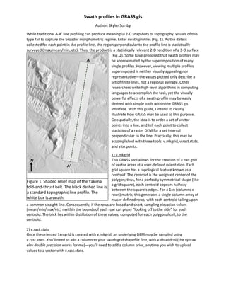
  • 1. This and more at my website: https://sites.google.com/site/sorsbysj/ LinkedIn: https://www.linkedin.com/in/skylersorsby Swath profiles in GRASS gis Author: Skyler Sorsby While traditional A-A’ line profiling can produce meaningful 2-D snapshots of topography, visuals of this type fail to capture the broader morphometric regime. Enter swath profiles (Fig. 1). As the data is collected for each point in the profile line, the region perpendicular to the profile line is statistically surveyed (max/mean/min, etc). Thus, the product is a statistically relevant 2-D rendition of a 3-D surface (Fig. 2). Some have proposed that swath profiles may be approximated by the superimposition of many single profiles. However, viewing multiple profiles superimposed is neither visually appealing nor representative—the values plotted only describe a set of finite lines, not a regional average. Other researchers write high-level algorithms in computing languages to accomplish the task, yet the visually powerful effects of a swath profile may be easily derived with simple tools within the GRASS gis interface. With this guide, I intend to clearly illustrate how GRASS may be used to this purpose. Geospatially, the idea is to order a set of vector points into a line, and tell each point to collect statistics of a raster DEM for a set interval perpendicular to the line. Practically, this may be accomplished with three tools: v.mkgrid, v.rast.stats, and v.to.points. 1) v.mkgrid This GRASS tool allows for the creation of a nxn grid of vector areas at a user-defined orientation. Each grid square has a topological feature known as a centroid. The centroid is the weighted center of the polygon; thus, for a perfectly symmetrical shape (like a grid square), each centroid appears halfway between the square’s edges. For a 1xn (columns x rows) matrix, this generates a single-column array of n user-defined rows, with each centroid falling upon a common straight line. Consequently, if the rows are broad and short, sampling elevation values (mean/min/max/etc) nwithin the bounds of each row can proxy “looking off to the side” for each centroid. The trick lies within distillation of these values, computed for each polygonal cell, to the centroid. 2) v.rast.stats Once the oriented 1xn grid is created with v.mkgrid, an underlying DEM may be sampled using v.rast.stats. You’ll need to add a column to your swath grid shapefile first, with v.db.addcol (the syntax elev double precision works for me)—you’ll need to add a column prior, anytime you wish to upload values to a vector with v.rast.stats. Figure 1. Shaded relief map of the Yakima fold-and-thrust belt. The black dashed line is a standard topographic line profile. The white box is a swath. N A A’
  • 2. This and more at my website: https://sites.google.com/site/sorsbysj/ LinkedIn: https://www.linkedin.com/in/skylersorsby Figure 2. Elevation profiles from the map in figure 1. The black and gray are the swath profile; the white dashed line is a line profile. 3) v.to.points When statistics have been assigned to each cell in the vector grid, these values may be distilled to the centroid, creating a new vector point file in the process. This is accomplished by using v.to.points— although documentation hints that this tool is meant for generating points along a line (not the case for us). This problem may be circumnavigated by checking the “centroids” box under the “feature type” heading. The result will be a shapefile of points, each point containing the max/mean/min/etc statistics for elevation of the topography immediately adjacent. Now, the only missing attribute is distance along the profile. Since each grid square was the same height and each centroid was centered vertically within each grid square, the distance between the points is simply the height of each grid square. Accordingly, distance will be a column of linearly-progressing values, easily auto-generated in Excel. 4) v.out.ogr The final step is to export your point shapefile to Excel as a .csv file, for auto-generation of a distance column and plotting. This tool may be finicky at times, sometimes requiring an entire file pathway to save to, others requiring only a name with which to label the containing folder (which will be placed in your ‘Users’ folder on the C:// drive). 5) Once you’ve exported your elevation graph of min/mean/max elevation from Excel as a pdf, you may easily augment it in a vector editing program like Inkscape (freeware) or Adobe Illustrator (certainly not freeware). In Inkscape, I’ve found that the easiest way to create a “filled” min/max envelope (see Fig. 2) is to make the min/max lines very narrow, connect them with two short vertical segments of the same color (to close the area), and use the paint bucket tool to give the area some pale color. In Illustrator, this task is much easier, as closing the area with two vertical lines automatically registers the shape as a polygon, whose interior “fill” may be set to any color you wish (no paint bucket tool involved-you get what you pay for!). 6) In the event that you’re working with data in a different coordinate system (say, you have a file of vector points along the course of a stream, with distance calculated for each point along the length of the stream—a curvy path), and you need to place your elevation swath profile into those coordinates. A A’
  • 3. This and more at my website: https://sites.google.com/site/sorsbysj/ LinkedIn: https://www.linkedin.com/in/skylersorsby The workflow is the same as above, but involves creation of a second grid, the same height and corner coordinates, but with much longer rows (to “reach out” orthogonal to the profile line and capture the values of the other point shapefile whose coordinates you’re attempting to reach into). Here is a simplified workflow for placing the swath profile into the coorinates of an adjacent river, for example, to compare the long profile with topographic relief: 1) Have a raster of river points, each point containing distance along the river (you may get a raster of river lines with the r.watershed, convert the raster to vector lines with r.to.vect, get rid of everything except your main channel with the digitizer tool, convert to raster points with v.to.rast (make sure it’s binary—river has a value of 1, else=NULL), multiply by the output of r.stream.distance to get a raster image of distance along the stream). 2) Create, as before a 1xn grid polygon for the swath profile with v.mkgrid (n is the number of rows you want) 3) Create another 1xn grid, VERY WIDE, such that the rows line up exactly vertically , but extend laterally completely across any river points with v.mkgrid 4) Convert the river points to a raster, if you haven’t done this already each cell containing distance values, with v.to.rast 5) Use v.rast.stats to get the mean distance for each row of the extended polygon (may have to use the Tk/Tcl GUI for GRASS—my python GUI seems buggy for this tool). 6) Use v.rast.stats to get the elevation statistics for each row of your swath polygon (as you did before). 7) Distill the swath rows to points with v.to.points, as you did before. 8) Use v.to.rast to convert the extended polygon to a raster with mean distance values (still by row) 9) Use v.what.rast to sample the extended polygon’s raster and obtain the mean river distance values for each row in the normal swath polygon. The basic premise is this: After creating your swath profile, you want to attach a “distance along the river” coordinate to each elevation—say, to compare structural relief of a linear set of features with a river’s long profile (and geometry), which certainly ISN’T linear. To do this, you’ll rasterize the river distance column of your river shapefile (points, I’m assuming), such that a new one column/many row grid oriented the same way as your swath grid but extending far beyond, can capture the mean values orthogonal to the swath. The extended grid, having captured the mean river distance, is now rasterized. The key is that the rasterization has now deposited this orthogonal mean river distance beneath the centroids of the original swath—effectively “reaching out and pulling in orthogonal river distance”. Using some sort of out-of-the-box spatial joining technique will not work as a substitute.
  • 4. This and more at my website: https://sites.google.com/site/sorsbysj/ LinkedIn: https://www.linkedin.com/in/skylersorsby Figure 3. Map showing the original swath (the narrow grid), the wider swath (whose sole purpose is to sample river distances, to relaty to the original swath). When the river distances are used, rather than the straight-line profile distance, the original swath will align with river-parallel features (useful for contrasting with changes in planform and geometry as topographic features are crossed). Figure 4. A pseudo “swath profile”, made from superimposing adjacent line profiles. Needless to say, it’s messier and less statistically relevant than a real swath. , , River points containing downstream distance Centroids to which swath values are distilled Large swath grid, to capture river distances for profile Original swath
  • 5. This and more at my website: https://sites.google.com/site/sorsbysj/ LinkedIn: https://www.linkedin.com/in/skylersorsby