Fundamentals of biomechanics

Applications of Statics to Biomechanics
5
5.1 Skeletal Joints
The human body is rigid in the sense that it can maintain a
posture, and flexible in the sense that it can change its
posture and move. The flexibility of the human body is due
primarily to the joints, or articulations, of the skeletal sys-
tem. The primary function of joints is to provide mobility to
the musculoskeletal system. In addition to providing mobil-
ity, a joint must also possess a degree of stability. Since
different joints have different functions, they possess vary-
ing degrees of mobility and stability. Some joints are
constructed so as to provide optimum mobility. For example,
the construction of the shoulder joint (ball-and-socket)
enables the arm to move in all three planes (triaxial motion).
However, this high level of mobility is achieved at the
expense of reduced stability, increasing the vulnerability of
the joint to injuries, such as dislocations. On the other hand,
the elbow joint provides movement primarily in one plane
(uniaxial motion), but is more stable and less prone to
injuries than the shoulder joint. The extreme case of
increased stability is achieved at joints that permit no rela-
tive motion between the bones constituting the joint. The
contacting surfaces of the bones in the skull are typical
examples of such joints.
The joints of the human skeletal system may be classified
based on their structure and/or function. Synarthrodial joints,
such as those in the skull, are formed by two tightly fitting
bones and do not allow any relative motion of the bones
forming them. Amphiarthrodial joints, such as those between
the vertebrae, allow slight relative motions, and feature an
intervening substance (a cartilaginous or ligamentous tissue)
whose presence eliminates direct bone-to-bone contact. The
third and mechanically most significant type of articulations
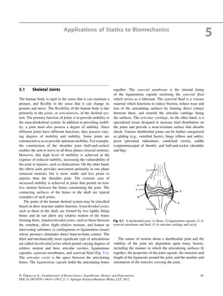
are called diarthrodial joints which permit varying degrees of
relative motion and have articular cavities, ligamentous
capsules, synovial membranes, and synovial fluid (Fig. 5.1).
The articular cavity is the space between the articulating
bones. The ligamentous capsule holds the articulating bones
together. The synovial membrane is the internal lining
of the ligamentous capsule enclosing the synovial fluid
which serves as a lubricant. The synovial fluid is a viscous
material which functions to reduce friction, reduce wear and
tear of the articulating surfaces by limiting direct contact
between them, and nourish the articular cartilage lining
the surfaces. The articular cartilage, on the other hand, is a
specialized tissue designed to increase load distribution on
the joints and provide a wear-resistant surface that absorbs
shock. Various diarthrodial joints can be further categorized
as gliding (e.g., vertebral facets), hinge (elbow and ankle),
pivot (proximal radioulnar), condyloid (wrist), saddle
(carpometacarpal of thumb), and ball-and-socket (shoulder
and hip).
The nature of motion about a diarthrodial joint and the
stability of the joint are dependent upon many factors,
including the manner in which the articulating surfaces fit
together, the properties of the joint capsule, the structure and
length of the ligaments around the joint, and the number and
orientation of the muscles crossing the joint.
Fig. 5.1 A diarthrodial joint: (1) Bone, (2) ligamentous capsule, (3, 4)
synovial membrane and fluid, (5, 6) articular cartilage and cavity
N. O¨ zkaya et al., Fundamentals of Biomechanics: Equilibrium, Motion, and Deformation,
DOI 10.1007/978-1-4614-1150-5_5, # Springer Science+Business Media, LLC 2012
61

5.2 Skeletal Muscles
In general, there are over 600 muscles in the human body,
accounting for about 45
of the total body weight.
There are three types of muscles: cardiac, smooth, and
skeletal. Cardiac muscle is the contractive tissue found in
the heart that pumps the blood for circulation. Smooth mus-
cle is found in the stomach, intestinal tracts, and the walls of
blood vessels. Skeletal muscle is connected to the bones of
the body and when contracted, causes body segments to
move.
Movement of human body segments is achieved as a
result of forces generated by skeletal muscles that convert
chemical energy into mechanical work. The structural
unit of skeletal muscle is the muscle fiber, which is com-
posed of myofibrils. Myofibrils are made up of actin and
myosin filaments. Muscles exhibit viscoelastic material
behavior. That is, they have both solid and fluid-like
material properties. Muscles are elastic in the sense that
when a muscle is stretched and released it will resume
its original (unstretched) size and shape. Muscles are vis-
cous in the sense that there is an internal resistance to
motion.
A skeletal muscle is attached, via soft tissues such as
aponeuroses and/or tendons, to at least two different bones
controlling the relative motion of one segment with respect
to the other. When its fibers contract under the stimulation of
a nerve, the muscle exerts a pulling effect on the bones to
which it is attached. Contraction is a unique property of the
muscle tissue. In engineering mechanics, contraction implies
shortening under compressive forces. In muscle mechanics,
contraction can occur as a result of muscle shortening or
muscle lengthening, or it can occur without any change in
the muscle length. Furthermore, the result of a muscle con-
traction is always tension: a muscle can only exert a pull.
Muscles cannot exert a push.
There are various types of muscle contractions: a concen-
tric contraction occurs simultaneously as the length of
the muscle decreases (e.g., the biceps during flexion of the
forearm); a static contraction occurs while muscle length
remains constant (the biceps when the forearm is flexed and
held without any movement); and an eccentric contraction
occurs as the length of the muscle increases (the biceps
during the extension of the forearm). A muscle can cause
movement only while its length is shortening (concentric
contraction). If the length of a muscle increases during a
particular activity, then the tension generated by the muscle
contraction is aimed at controlling the movement of the
body segments associated with that muscle (excentric con-
traction). If a muscle contracts but there is no segmental
motion, then the tension in the muscle balances the effects
of applied forces such as those due to gravity (isometric
contraction).
The skeletal muscles can also be named according to the
functions they serve during a particular activity. For exam-
ple, a muscle is called agonist if it causes movement through
the process of its own contraction. Agonist muscles are the
primary muscles responsible for generating a specific move-
ment. An antagonist muscle opposes the action of another
muscle. Synergic muscle is that which assists the agonist
muscle in performing the same joint motion.
5.3 Basic Considerations
In this chapter, we want to apply the principles of statics
to investigate the forces involved in various muscle
groups and joints for various postural positions of the
human body and its segments. Our immediate purpose is to
provide answers to questions such as: what tension must
the neck extensor muscles exert on the head to support
the head in a specified position? When a person bends,
what would be the force exerted by the erector spinae on
the fifth lumbar vertebra? How does the compression at
the elbow, knee, and ankle joints vary with externally
applied forces and with different segmental arrangements?
How does the force on the femoral head vary with loads
carried in the hand? What are the forces involved in various
muscle groups and joints during different exercise
conditions?
The forces involved in the human body can be grouped as
internal and external. Internal forces are those associated
with muscles, ligaments, and tendons, and at the joints.
Externally applied forces include the effect of gravitational
acceleration on the body or on its segments, manually and/or
mechanically applied forces on the body during exercise and
stretching, and forces applied to the body by prostheses and
implements. In general, the unknowns in static problems
involving the musculoskeletal system are the joint reaction
forces and muscle tensions. Mechanical analysis of a joint
requires that we know the vector characteristics of tension
in the muscle including the proper locations of muscle
attachments, the weights or masses of body segments, the
centers of gravity of the body segments, and the anatomical
axis of rotation of the joint.
5.4 Basic Assumptions and Limitations
The complete analysis of muscle forces required to sustain
various postural positions is difficult because of the complex
arrangement of muscles within the human body and because
of limited information. In general, the relative motion of
62 5 Applications of Statics to Biomechanics

body segments about a given joint is controlled by more than
one muscle group. To be able to reduce a specific problem of
biomechanics to one that is statically determinate and apply
the equations of equilibrium, only the muscle group that is
the primary source of control over the joint can be taken into
consideration. Possible contributions of other muscle groups
to the load-bearing mechanism of the joint must be ignored.
Note however that approximations of the effect of other
muscles may be made by considering their cross-sectional
areas and their relative positions in relation to the joint. Also,
if the phasic activity of muscles is known via some
experiments such as the electromyography (EMG)
measurements of muscle signals, then the tension in differ-
ent muscle groups may be estimated.
To apply the principles of statics to analyze the mechan-
ics of human joints, we shall adopt the following
assumptions and limitations:
• The anatomical axes of rotation of joints are known.
• The locations of muscle attachments are known.
• The line of action of muscle tension is known.
• Segmental weights and their centers of gravity are
known.
• Frictional factors at the joints are negligible.
• Dynamic aspects of the problems will be ignored.
• Only two-dimensional problems will be considered.
These analyses require that the anthropometric data about
the segment to be analyzed must be available. For this
purpose, there are tables listing anthropometric information
including average weights, lengths, and centers of gravity of
body segments. See Chaffin et al. (1999), Roebuck (1995),
and Winter (2004) for a review of the anthropometric data
available.
It is clear from this discussion that we shall analyze
certain idealized problems of biomechanics. Based on the
results obtained and experience gained, these models may be
expanded by taking additional factors into consideration.
However, a given problem will become more complex as
more factors are considered.
In the following sections, the principles of statics are
applied to analyze forces involved at and around the major
joints of the human body. First, a brief functional anatomy of
each joint and related muscles is provided, and specific bio-
mechanical problems are constructed. For a more complete
discussion about the functional anatomy of joints, see texts
such as Nordin and Frankel (2012) and Thompson (1989).
Next, an analogy is formed between muscles, bones, and
human joints, and certain mechanical elements such as
cables, beams, and mechanical joints. This enables us to
construct a mechanical model of the biological
system under consideration. Finally, the procedure outlined
in section “Procedure to Analyze Systems in Equilibrium”
of Chap. 4 is applied to analyze the mechanical model
thus constructed. See LeVeau (1992) for additional examples
of the application of the principles of statics to biomechanics.
5.5 Mechanics of the Elbow
The elbow joint is composed of three separate articulations
(Fig. 5.2). The humeroulnar joint is a hinge (ginglymus)
joint formed by the articulation between the spool-shaped
trochlea of the distal humerus and the concave trochlear
fossa of the proximal ulna. The structure of the humeroulnar
joint is such that it allows only uniaxial rotations, confining
the movements about the elbow joint to flexion (movement
of the forearm toward the upper arm) and extension (move-
ment of the forearm away from the upper arm). The
humeroradial joint is also a hinge joint formed between the
capitulum of the distal humerus and the head of the radius.
The proximal radioulnar joint is a pivot joint formed by the
head of the radius and the radial notch of the proximal ulna.
This articulation allows the radius and ulna to undergo
relative rotation about the longitudinal axis of one or the
other bone, giving rise to pronation (the movement experi-
enced while going from the palm-up to the palm-down) or
supination (the movement experienced while going from the
palm-down to the palm-up).
The muscles coordinating and controlling the movement
of the elbow joint are illustrated in Fig. 5.3. The biceps
brachii muscle is a powerful flexor of the elbow joint, par-
ticularly when the elbow joint is in a supinated position. It is
the most powerful supinator of the forearm. On the distal
side, the biceps is attached to the tuberosity of the radius, and
on the proximal side, it has attachments at the top of the
coracoids process and upper lip of the glenoid fossa. Another
important flexor is the brachialis muscle which, regardless of
forearm orientation, has the ability to produce elbow flexion.
Fig. 5.2 Bones of the elbow:
(1) humerus, (2) capitulum,
(3) trochlea, (4) radius, (5) ulna
5.5 Mechanics of the Elbow 63

It is then the strongest flexor of the elbow. It has attachments
at the lower half of the anterior portion of the humerus and
the coronoid process of the ulna. Since it does not inset on
the radius, it cannot participate in pronation or supination.
The most important muscle controlling the extension
movement of the elbow is the triceps brachii muscle. It has
attachments at the lower head of the glenoid cavity of the
scapula, the upper half of the posterior surface of the
humerus, the lower two thirds of the posterior surface of
the humerus, and the olecranon process of the ulna. Prona-
tion and supination movements of the forearm are performed
by the pronator teres and supinator muscles, respectively.
The pronator teres is attached to the lower part of the inner
condyloid ridge of the humerus, the medial side of the
ulna, and the middle third of the outer surface of the radius.
The supinator muscle has attachments at the outer condyloid
ridge of the humerus, the neighboring part of the ulna and the
outer surface of the upper third of the radius.
Common injuries of the elbow include fractures and
dislocations. Fractures usually occur at the epicondyles
of the humerus and the olecranon process of the ulna.
Another group of elbow injuries are associated with overuse,
which causes an inflammatory process of the tendons of an
elbow that has been damaged by repetitive motions. These
include tennis elbow and golfer’s elbow syndromes.
Example 5.1 Consider the arm shown in Fig. 5.4. The elbow
is flexed to a right angle and an object is held in the hand.
The forces acting on the forearm are shown in Fig. 5.5a, and
the free-body diagram of the forearm is shown on a
mechanical model in Fig. 5.5b. This model assumes that
the biceps is the major flexor and that the line of action of
the tension (line of pull) in the biceps is vertical.
Point O designates the axis of rotation of the elbow joint,
which is assumed to be fixed for practical purposes. Point A
is the attachment of the biceps muscle on the radius, point B
is the center of gravity of the forearm, and point C is a point
on the forearm that lies along a vertical line passing through
the center of gravity of the weight in the hand. The distances
between point O and points A, B, and C are measured as a, b,
and c, respectively. Wo is the weight of the object held in the
hand and W is the total weight of the forearm. FM is the
magnitude of the force exerted by the biceps on the radius,
and FJ is the magnitude of the reaction force at the elbow
joint. Notice that the line of action of the muscle force is
assumed to be vertical. The gravitational forces are vertical
as well. Therefore, for the equilibrium of the lower arm, the
line of action of the joint reaction force must also be vertical
(a parallel force system).
Fig. 5.3 Muscles of the elbow: (1) biceps, (2) brachioradialis, (3)
brachialis, (4) pronator teres, (5) triceps brachii, (6) anconeus, (7)
supinator
Fig. 5.4 Example 5.1
Fig. 5.5 Forces acting on the lower arm

The task in this example is to determine the magnitudes of
the muscle tension and the joint reaction force at the elbow.
Solution
We have a parallel force system, and the unknowns are the
magnitudes FM and FJ of the muscle and joint reaction
forces. Considering the rotational equilibrium of the forearm
about the elbow joint and assuming the (cw) direction is
positive:
X
Mo ¼ 0:
That is, cWo þ bW À aFM ¼ 0:
Then FM ¼
1
a
ðbW þ cWoÞ: (i)
For the translational equilibrium of the forearm in the y
direction,
X
Fy ¼ 0:
That is, À FJ þ FM À W À Wo ¼ 0:
Then FJ ¼ FM À W À Wo: (ii)
For given values of geometric parameters a, b, and c, and
weights W and Wo, Eqs. (i) and (ii) can be solved for the
magnitudes of the muscle and joint reaction forces. For
example, assume that these parameters are given as
follows: a ¼ 4cm; b ¼ 15cm; c ¼ 35cm; W ¼ 20N,
and Wo ¼ 80N. Then from Eqs. (i) and (ii):
FM ¼
1
0:04
ð0:15Þð20Þ þ ð0:35Þð80Þ½ Š ¼ 775 N ðþyÞ:
FJ ¼ 775 À 20 À 80 ¼ 675 N ðÀyÞ:
Remarks
• The numerical results indicate that the force exerted by
the biceps muscle is about ten times larger than the
weight of the object held in the position considered.
Relative to the axis of the elbow joint, the length a of
the lever arm of the muscle force is much smaller than the
length c of the lever arm enjoyed by the load held in the
hand. The smaller the lever arm, the greater the muscle
tension required to balance the clockwise rotational effect
of the load about the elbow joint. Therefore, during
lifting, it is disadvantageous to have a muscle attachment
close to the elbow joint. However, the closer the muscle is
to the joint, the larger the range of motion of elbow
flexion–extension, and the faster the distal end (hand) of
the forearm can reach its goal of moving toward the upper
arm or the shoulder.
• The angle between the line of action of the muscle force
and the long axis of the bone upon which the muscle force
is exerted is called the angle of pull and it is critical in
determining the effectiveness of the muscle force. When
the lower arm is flexed to a right angle, the muscle tension
has only a rotational effect on the forearm about the
elbow joint, because the line of action of the muscle
force is at a right angle with the longitudinal axis of
the forearm. For other flexed positions of the forearm,
the muscle force can have a translational (stabilizing or
sliding) component as well as a rotational component.
Assume that the linkage system shown in Fig. 5.6a
illustrates the position of the forearm relative to the upper
arm. n designates a direction perpendicular (normal) to
the long axis of the forearm and t is tangent to it. Assum-
ing that the line of action of the muscle force remains
parallel to the long axis of the humerus, FM can be
decomposed into its rectangular components FMn and
FMt. In this case, FMn is the rotational (rotatory) compo-
nent of the muscle force because its primary function is to
rotate the forearm about the elbow joint. The tangential
component FMt of the muscle force acts to compress the
elbow joint and is called the stabilizing component of the
Fig. 5.6 Rotational (FMn) and stabilizing or sliding (FMt) components
of the muscle force
5.5 Mechanics of the Elbow 65

muscle force. As the angle of pull approaches 90
, the
magnitude of the rotational component of the muscle
force increases while its stabilizing component decreases,
and less and less energy is “wasted” to compress the
elbow joint. As illustrated in Fig. 5.6b, the stabilizing
role of FMt changes into a sliding or dislocating role
when the angle between the long axes of the forearm
and upper arm becomes less than 90
.
• The elbow is a diarthrodial (synovial) joint. A ligamentous
capsule encloses an articular cavity which is filled with
synovial fluid. Synovial fluid is a viscous material whose
primary function is to lubricate the articulating surfaces,
thereby reducing the frictional forces that may develop
while one articulating surface slides over the other. The
synovial fluid also nourishes the articulating cartilages. A
commonpropertyoffluidsisthattheyexert pressures(force
per unit area) that are distributed over the surfaces they
touch. The fluid pressure always acts in a direction toward
and perpendicular to the surface it touches having a com-
pressiveeffectonthe surface.Notethat inFig.5.7, the small
vectors indicating the fluid pressure have components in the
horizontal and vertical directions. We determined that the
joint reaction force at the elbow acts vertically downward
on the ulna. This implies that the horizontal components of
these vectors cancel out (i.e., half pointing to the left and
half pointing to the right), but their vertical components (on
the ulna, almost all of them are pointing downward) add up
to form the resultant force FJ (shown with a dashed arrow in
Fig.5.7c).Therefore,thejointreactionforceFJ corresponds
to the resultant of the distributed force system (pressure)
applied through the synovial fluid.
• The most critical simplification made in this example is
that the biceps was assumed to be the single muscle group
responsible for maintaining the flexed configuration of
the forearm. The reason for making such an assumption
was to reduce the system under consideration to one that
is statically determinate. In reality, in addition to the
biceps, the brachialis and the brachioradialis are primary
elbow flexor muscles.
Consider the flexed position of the arm shown in
Fig. 5.8a. The free-body diagram of the forearm is shown
in Fig. 5.8b. FM1, FM2, and FM3 are the magnitudes of the
forces exerted on the forearm by the biceps, the brachialis,
and the brachioradialis muscles with attachments at points
A1, A2, and A3, respectively. Let y1, y2, and y3 be the angles
that the biceps, the brachialis, and the brachioradialis
muscles make with the long axis of the lower arm. As
compared to the single-muscle system which consisted of
two unknowns (FM and Fj), the analysis of this three-muscle
system is quite complex. First of all, this is not a simple
parallel force system. Even if we assume that the locations of
muscle attachments (A1,A2, and A3), their angles of pull (y1,
y2, and y3) and the lengths of their moment arms (a1, a2, and
a3) as measured from the elbow joint are known, there are
still five unknowns in the problem (FM1, FM2, FM3, Fj, and b,
where the angle b is an angle between Fj and the long axes of
the forearm). The total number of equations available from
statics is three:
X
Mo ¼ 0 : a1FM1 þa2FM2 þa3FM3 ¼ bW þcWo: (iii)
Fig. 5.8 Three-muscle systemFig. 5.7 Explaining the joint reaction force at the elbow

X
Fx ¼ 0 : FJx ¼ FM1x þ FM2x þ FM3x: (iv)
X
Fy ¼ 0 : FJy ¼ FM1y þ FM2y þ FM3y À W À Wo: (v)
Note that once the muscle forces are determined, Eqs. (iv)
and (v) will yield the components of the joint reaction force
FJ. As far as the muscle forces are concerned, we have only
Eq. (iii) with three unknowns. In other words, we have a
statically indeterminate problem. To obtain a unique solution,
we need additional information relating FM1, FM2, and FM3.
There may be several approaches to the solution of this
problem. The criteria for estimating the force distribution
among different muscle groups may be established by (1)
using cross-sectional areas of muscles, (2) using EMG
measurements of muscle signals, and (3) applying certain
optimization techniques. It may be assumed that each mus-
cle exerts a force proportional to its cross-sectional area.
If S1, S2, and S3 are the cross-sectional areas of the biceps,
the brachialis, and the brachioradialis, then this criteria may
be applied by expressing muscle forces in the following
manner:
FM2 ¼ k21 FM1 with k21 ¼
S2
S1
: (vi)
FM3 ¼ k31 FM1 with k31 ¼
S3
S1
: (vii)
If constants k21 and k31 are known, then Eqs. (vi) and (vii)
can be substituted into Eq. (iii), which can then be solved for
FM1:
FM1 ¼
b W þ c Wo
a1 þ a2 k21 þ a3 k31
:
Substituting FM1 back into Eqs. (vi) and (vii) will then
yield the magnitudes of the forces in the brachialis and the
brachioradialis muscles. The values of k21 and k31 may also be
estimated by using the amplitudes of muscle EMG signals.
This statically indeterminate problem may also be solved
by considering some optimization techniques. If the purpose
is to accomplish a certain task (static or dynamic) in the most
efficient manner, then the muscles of the body must act to
minimize the forces exerted, the moments about the joints (for
dynamic situations), and/or the work done by the muscles.
The question is, what force distribution among the various
muscles facilitates the maximum efficiency?
5.6 Mechanics of the Shoulder
The bony structure and the muscles of the shoulder complex
are illustrated in Figs. 5.9 and 5.10. The shoulder forms the
base for all upper extremity movements. The complex
structure of the shoulder can be divided into two: the shoul-
der joint and the shoulder girdle.
The shoulder joint, also known as the glenohumeral
articulation, is a ball-and-socket joint between the nearly
hemispherical humeral head (ball) and the shallowly con-
cave glenoid fossa (socket) of the scapula. The shallowness
of the glenoid fossa allows a significant freedom of move-
ment of the humeral head on the articulating surface of the
glenoid. The movements allowed are in the sagittal plane,
flexion (movement of the humerus to the front—a forward
upward movement) and extension (return from flexion); in
Fig. 5.9 The shoulder: (1) sternoclavicular joint, (2) sternum, (3)
glenohumeral joint, (4) clavicle, (5) acromioclavicular joint, (6)
acromion process, (7) glenoid fossa, (8) scapula, (9) humerus
Fig. 5.10 Shoulder muscles: (1) deltoideus, (2) pectoralis minor, (3)
subscapularis, (4) pectoralis major, (5) trapezius, (6) infraspinatus and
teres minor, (7) latissimus dorsi, (8) levator scapulae, (9) supraspinatus,
(10) rhomboideus, (11) teres major
5.6 Mechanics of the Shoulder 67

the coronal plane, abduction (horizontal upward movement
of the humerus to the side) and adduction (return from
abduction); and in the transverse plane, outward rotation
(movement of the humerus around its long axis to the lateral
side) and inward rotation (return from outward rotation). The
conﬁguration of the articulating surfaces of the shoulder
joint also makes the joint more susceptible to instability
and injury, such as dislocation. The stability of the joint is
provided by the glenohumeral and coracohumeral ligaments,
and by the muscles crossing the joint. The major muscles of
the shoulder joint are deltoideus, supraspinatus, pectoralis
major, coracobrachialis, latissimus dorsi, teres major, teres
minor, infraspinatus, and subscapularis.
The bony structure of the shoulder girdle consists of
the clavicle (collarbone) and the scapula (shoulder blade).
The acromioclavicular joint is a small synovial articulation
between the distal clavicle and the acromion process of the
scapula. The stability of this joint is reinforced by the
coracoclavicular ligaments. The sternoclavicular joint is
the articulation between the manubrium of the sternum and
the proximal clavicle. The stability of this joint is enhanced
by the costoclavicular ligament. The acromioclavicular joint
and the sternoclavicular joint both have layers of cartilage,
called menisci, interposed between their bony surfaces.
There are four pairs of scapular movements: elevation
(movement of the scapula in the frontal plane) and depres-
sion (return from elevation), upward rotation (turning the
glenoid fossa upward and the lower medial border of the
scapula away from the spinal column) and downward rota-
tion (return from upward rotation), protraction (movement
of the distal end of the clavicle forward) and retraction
(return from protraction), and forward and backward rota-
tion (rotation of the scapula about the shaft of the clavicle).
Some of the main muscles that control and coordinate these
movements are the trapezius, levator scapulae, rhomboid,
pectoralis minor, serratus anterior, and subclavius.
Example 5.2 Consider a person strengthening the shoulder
muscles by means of dumbbell exercises. Figure 5.11
illustrates the position of the left arm when the arm is fully
abducted to horizontal. The free-body diagram of the arm is
shown in Fig. 5.12 along with a mechanical model of the
arm. Also in Fig. 5.12, the forces acting on the arm are
resolved into their rectangular components along the hori-
zontal and vertical directions. Point O corresponds to
the axis of rotation of the shoulder joint, point A is where
the deltoid muscle is attached to the humerus, point B is the
center of gravity of the entire arm, and point C is the center
of gravity of the dumbbell. W is the weight of the arm, Wo is
the weight of the dumbbell, FM is the magnitude of the
tension in the deltoid muscle, and Fj is the joint reaction
force at the shoulder. The resultant of the deltoid muscle
force makes an angle y with the horizontal. The distances
between point O and points A, B, and C are measured as a, b,
and c, respectively.
Determine the magnitude FM of the force exerted by the
deltoid muscle to hold the arm at the position shown. Also
determine the magnitude and direction of the reaction force
at the shoulder joint in terms of speciﬁed parameters.
Solution
With respect to the xy coordinate frame, the muscle and joint
reaction forces have two components while the weights of
the arm and the dumbbell act in the negative y direction. The
components of the muscle force are
FMx ¼ FM cos y ðÀxÞ: (i)
FMy ¼ FM sin y ðþyÞ: (ii)
Fig. 5.11 The arm is abducted to horizontal
Fig. 5.12 Forces acting on the arm and a mechanical model
representing the arm

Components of the joint reaction force are
FJx ¼ FJ cos b ðþxÞ: (iii)
FJy ¼ FJ sin b ðÀyÞ (iv)
b is the angle that the joint reaction force makes with the
horizontal. The line of action and direction (in terms of y)
of the force exerted by the muscle on the arm are known.
However, the magnitude FM of the muscle force, the magni-
tude Fj, and the direction (b) of the joint reaction force
are unknowns. We have a total of three unknowns, FM, Fj,
and b (or FM, FJx, and FJy). To be able to solve this two-
dimensional problem, we have to utilize all three equilib-
rium equations.
First, consider the rotational equilibrium of the arm about
the shoulder joint at point O. The joint reaction force
produces no torque about point O because its line of action
passes through it. For practical purposes, we can neglect the
possible contribution of the horizontal component of the
muscle force to the moment generated about point O by
assuming that its line of action also passes through point
O. Note that this is not a critical or necessary assumption to
solve this problem. If we knew the length of its moment arm
(i.e., the vertical distance between O and A), we could easily
incorporate the torque generated by FMx about point O into
the analysis. Under these considerations, there are only three
moment producing forces about point O. For the rotational
equilibrium of the arm, the net moment about point O must
be equal to zero. Taking counterclockwise moments to be
positive:
X
Mo ¼ 0 : a FMy À b W À c Wo ¼ 0
FMy ¼
1
a
ðb W þ c WoÞ: (v)
For given a; b; c; W, and Wo, Eq. (v) can be used to
determine the vertical component of the force exerted by the
deltoid muscle. Equation, (ii) can now be used to determine
the total force exerted by the muscle:
FM ¼
FMy
sin y
: (vi)
Knowing FM, Eq. (i) will yield the horizontal component
of the tension in the muscle:
FMx ¼ FM cos y: (vii)
The components of the joint reaction force can be deter-
mined by considering the translational equilibrium of the
arm in the horizontal and vertical directions:
X
Fx ¼ 0 thatis, FJx ÀFMx ¼ 0; then FJx ¼ FMx: (viii)
X
Fy ¼ 0 that is, À FJy þ FMy À W À Wo ¼ 0;
then FJy ¼ FMy À W À Wo: (ix)
Knowing the rectangular components of the joint reaction
force enables us to compute the magnitude of the force itself
and the angle its line of action makes with the horizontal:
FJ ¼
ffiffiffiffiffiffiffiffiffiffiffiffiffiffiffiffiffiffiffiffiffiffiffiffiffiffiffiffiffiffi
ðFJxÞ2
þ ðFJyÞ2
q
: (x)
b ¼ tanÀ1 FJy
FJx

: (xi)
Now consider that a ¼ 15 cm; b ¼ 30 cm;
c ¼ 60 cm; y ¼ 15
; W ¼ 40 N, and Wo ¼ 60 N. Then,
FMy ¼
1
0:15
ð0:30Þð40Þ þ ð0:60Þð60Þ½ Š ¼ 320 N ðþyÞ:
FM ¼
320
sin 15
¼ 1;236 N:
FMx ¼ ð1;236Þ ðcos 15
Þ ¼ 1;194 N ðÀxÞ:
FJx ¼ 1;194 N ðþxÞ:
FJy ¼ 320 À 40 À 60 ¼ 220 N ðÀyÞ:
FJ ¼
ffiffiffiffiffiffiffiffiffiffiffiffiffiffiffiffiffiffiffiffiffiffiffiffiffiffiffiffi
1;1942
þ 2202
q
¼ 1;214 N:
b ¼ tanÀ1 220
1;194

¼ 10
:
Remarks
• FMx is the stabilizing component and FMy is the rotational
component of the deltoid muscle. FMx is approximately
four times larger than FMy. A large stabilizing component
suggests that the horizontal position of the arm is not
stable, and that the muscle needs to exert a high horizon-
tal force to stabilize it.
• The human shoulder is very susceptible to injuries. The
most common injuries are dislocations of the shoulder
joint and the fracture of the humerus. Since the socket of
the glenohumeral joint is shallow, the head of the
humerus is relatively free to rotate about the articulating
surface of the glenoid fossa. This freedom of movement
is achieved, however, by reduced joint stability. The
humeral head may be displaced in various ways,
depending on the strength or weakness of the muscular
and ligamentous structure of the shoulder, and depending
5.6 Mechanics of the Shoulder 69

on the physical activity. Humeral fractures are another
common type of injuries. The humerus is particularly
vulnerable to injuries because of its unprotected
configuration.
• Average ranges of motion of the arm about the shoulder
joint are 230
during flexion–extension, and 170
in both
abduction–adduction and inward–outward rotation.
5.7 Mechanics of the Spinal Column
The human spinal column is the most complex part of the
human musculoskeletal system. The principal functions of
the spinal column are to protect the spinal cord; to support
the head, neck, and upper extremities; to transfer loads from
the head and trunk to the pelvis; and to permit a variety of
movements. The spinal column consists of the cervical
(neck), thoracic (chest), lumbar (lower back), sacral, and
coccygeal regions. The thoracic and lumbar sections of the
spinal column make up the trunk. The sacral and coccygeal
regions are united with the pelvis and can be considered
parts of the pelvic girdle.
The vertebral column consists of 24 intricate and com-
plex vertebrae (Fig. 5.13). The articulations between the
vertebrae are amphiarthrodial joints. A fibrocartilaginous
disk is interposed between each pair of vertebrae. The pri-
mary functions of these intervertebral disks are to sustain
loads transmitted from segments above, act as shock
absorbers, eliminate bone-to-bone contact, and reduce the
effects of impact forces by preventing direct contact between
the bony structures of the vertabrae. The articulations of
each vertebra with the adjacent vertabrae permit movement
in three planes, and the entire spine functions like a single
ball-and-socket joint. The structure of the spine allows a
wide variety of movements including flexion–extension,
lateral flexion, and rotation.
Two particularly important joints of the spinal column
are those with the head (occiput bone of the skull) and the
first cervical vertebrae, atlas, and the atlas and the second
vertebrae, the axis. The atlantooccipital joint is the union
between the first cervical vertebra (the atlas) and the occipi-
tal bone of the head. This is a double condyloid joint and
permits movements of the head in the sagittal and frontal
planes. The atlantoaxial joint is the union between the atlas
and the odontoid process of the head. It is a pivot joint,
enabling the head to rotate in the transverse plane. The
muscle groups providing, controlling, and coordinating
the movement of the head and the neck are the preverte-
brals (anterior), hyoids (anterior), sternocleidomastoid
(anterior–lateral), scalene (lateral), levator scapulae (lat-
eral), suboccipitals (posterior), and spleni (posterior).
The spine gains its stability from the intervertebral discs
and from the surrounding ligaments and muscles (Fig. 5.14).
The discs and ligaments provide intrinsic stability, and the
muscles supply extrinsic support. The muscles of the spine
exist in pairs. The anterior portion of the spine contains
the abdominal muscles: the rectus abdominis, transverse
abdominus, external obliques, and internal obliques. These
muscles provide the necessary force for trunk flexion and
maintain the internal organs in proper position. There are
three layers of posterior trunk muscles: erector spinae,
semispinalis, and the deep posterior spinal muscle groups.
The primary function of the muscles located at the posterior
portion of the spine is to provide trunk extension. These
muscles also support the spine against the effects of gravity.
The quadratus lumborum muscle is important in lateral
trunk flexion. It also stabilizes the pelvis and lumbar spine.
Fig. 5.14 Selected muscles of
the neck and spine: (1) splenius,
(2) sternocleidomastoid,
(3) hyoid, (4) levator scapula,
(5) erector spinae, (6) obliques,
(7) rectus abdominis,
(8) transversus abdominis
Fig. 5.13 The spinal column:
(1) cervical vertebrae, (2) thoracic
vertebrae, (3) lumbar vertabrae,
(4) sacrum

The lateral flexion of the trunk results from the actions of the
abdominal and posterior muscles. The rotational movement
of the trunk is controlled by the simultaneous action of
anterior and posterior muscles.
The spinal column is vulnerable to various injuries. The
most severe injury involves the spinal cord, which is
immersed in fluid and protected by the bony structure.
Other critical injuries include fractured vertebrae and
herniated intervertebral disks. Lower back pain may also
result from strains in the lower regions of the spine.
Example 5.3 Consider the position of the head and the neck
shown in Fig. 5.15. Also shown are the forces acting on the
head. The head weighs W ¼ 50 N and its center of gravity is
located at point C. FM is the magnitude of the resultant force
exerted by the neck extensor muscles, which is applied on
the skull at point A. The atlantooccipital joint center is
located at point B. For this flexed position of the head, it is
estimated that the line of action of the neck muscle force
makes an angle y ¼ 30
and the line of action of the joint
reaction force makes an angle b ¼ 60
with the horizontal.
What tension must the neck extensor muscles exert to
support the head? What is the compressive force applied on
the first cervical vertebra at the atlantooccipital joint?
Solution
We have a three-force system with two unknowns:
magnitudes FM and Fj of the muscle and joint reaction forces.
Since the problem has a relatively complicated geometry, it is
convenient to utilize the condition that for a body to be in
equilibrium the force system acting on it must be either
concurrent or parallel. In this case, it is clear that the forces
involved do not form a parallel force system. Therefore, the
system of forces under consideration must be concurrent.
Recall that a system of forces is concurrent if the lines of
action of all forces have a common point of intersection.
In Fig. 5.15, the lines of action of all three forces acting
on the head are extended to meet at point O. In Fig. 5.16,
the forces W, FM, and FJ acting on the skull are translated to
point O, which is also chosen to be the origin of the xy
coordinate frame. The rectangular components of the muscle
and joint reaction forces in the x and y directions are
FMx ¼ FM cos y: (i)
FMy ¼ FM sin y: (ii)
FJx ¼ FJ cos b: (iii)
FJy ¼ FJ sin b: (iv)
The translational equilibrium conditions in the x and y
directions will yield
X
Fx ¼ 0 that is : ÀFJx þ FMx ¼ 0;
then FJx ¼ FMx: (v)
X
Fy ¼ 0 that is : ÀW À FMy þ FJy ¼ 0;
then FJy ¼ W þ FMy: (vi)
Substitute Eqs. (i) and (iii) into Eq. (v):
FJ cos b ¼ FM cos y: (vii)
Substitute Eqs. (ii) and (iv) into Eq. (vi):
FJ sin b ¼ W þ FM sin y (viii)
Substitute this equation into Eq. (viii), that is,
FM Â cos y
cos b
Â sin b ¼ W þ FM sin y;
Fig. 5.15 Forces on the skull form a concurrent system
Fig. 5.16 Components of the forces acting on the head
5.7 Mechanics of the Spinal Column 71

FM Â cos y tan b ¼ W þ FM sin y;
then
tan b ¼
W þ FM sin y
FM cos y
: (ix)
Equation (ix) can now be solved for the unknown muscle
force FM:
FM cos y tan b ¼ W þ FM sin y
FM ðcos y tan b À sin yÞ ¼ W
FM ¼
W
cos y tan b À sin y
: (x)
Equation (x) gives the tension in the muscle as a function
of the weight W of the head and the angles y and b that the
lines of action of the muscle and joint reaction forces make
with the horizontal. Substituting the numerical values of W,
y, and b will yield
FM ¼
50
ðcos 30Þ ðtan 60Þ À ð sin 30Þ
¼ 50 N:
From Eqs. (i) and (ii),
FMx ¼ ð50Þðcos 30
Þ ¼ 43 N ðþxÞ
FMy ¼ ð50Þðsin 30
Þ ¼ 25 N ðÀyÞ:
From Eqs. (v) and (vi),
FJx ¼ 43 N ðÀxÞ
FJy ¼ 50 þ 25 ¼ 75 N ðþyÞ:
The resultant of the joint reaction force can be computed
either from Eqs. (iii) or (iv). Using Eq. (iii)
FJ ¼
FJx
cos b
¼
43
cos 60
¼ 86 N:
Remarks
• The extensor muscles of the head must apply a force of
50 N to support the head in the position considered. The
reaction force developed at the atlantooccipital joint is
about 86 N.
• The joint reaction force can be resolved into two rectan-
gular components, as shown in Fig. 5.17. FJn is the
magnitude of the normal component of FJ compressing
the articulating joint surface, and FJt is the magnitude of
its tangential component having a shearing effect on the
joint surfaces. Forces in the muscles and ligaments of
the neck operate in a manner to counterbalance this
shearing effect.
Example 5.4 Consider the weight lifter illustrated in
Fig. 5.18, who is bent forward and lifting a weight Wo.
At the position shown, the athlete’s trunk is ﬂexed by an
angle y as measured from the upright (vertical) position.
The forces acting on the lower portion of the athlete’s
body are shown in Fig. 5.19 by considering a section passing
through the ﬁfth lumbar vertebra. A mechanical model of the
athlete’s lower body (the pelvis and legs) is illustrated in
Fig. 5.20 along with the geometric parameters of the prob-
lem under consideration. W is the total weight of the athlete,
W1 is the weight of the legs including the pelvis, ðW þ W0Þ
is the total ground reaction force applied to the athlete
through the feet (at point C), FM is the magnitude of the
resultant force exerted by the erector spinae muscles
supporting the trunk, and FJ is the magnitude of the com-
pressive force generated at the union (point O) of the sacrum
Fig. 5.17 Normal and shear components of the joint reaction force
Fig. 5.18 A weight lifter

and the ﬁfth lumbar vertebra. The center of gravity of the
legs including the pelvis is located at point B. Relative to
point O, the lengths of the lever arms of the muscle force,
lower body weight, and ground reaction force are measured
as a; b, and c, respectively.
Assuming that the line of pull of the resultant muscle
force exerted by the erector spinae muscles is parallel to
the trunk (i.e., making an angle y with the vertical), deter-
mine FM and FJ in terms of, b; c; y; W0; W1, and W.
Solution
In this case, there are three unknowns: FM, FJx, and FJy. The
lengths of the lever arms of the muscle force, ground reaction
force, andthe gravitational force of the legs including the pelvis
are given as measured from point O. Therefore, we can apply
the rotational equilibrium condition about point O to determine
the magnitude FM of the resultant force exerted by the erector
spinae muscles. Considering clockwise moments to be positive
X
Mo ¼ 0 : aFM þ bW1 À cðW þ W0Þ ¼ 0:
Solving this equation for FM will yield
FM ¼
cðW þ W0Þ À bW1
a
: (i)
For given numerical values of, b; c; y; W0; W1, and W,
Eq. (i) can be used to determine the magnitude of the
resultant muscle force. Once FM is calculated, its components
in the x and y directions can be determined using
FMx ¼ FM sin y: (ii)
FMy ¼ FM cos y: (iii)
The horizontal and vertical components of the reaction
force developed at the sacrum can now be determined by
utilizing the translational equilibrium conditions of the
lower body of the athlete in the x and y directions:
X
Fx ¼ 0 That is; FMx À FJx ¼ 0; then FJx ¼ FMx: (iv)
X
Fy ¼ 0 That is; FMy À FJy À W1 þ ðW þ W0Þ ¼ 0;
then FJy ¼ FMy þ W þ W0 À W1:
(v)
Assume that at an instant the athlete is bent so that his
trunk makes an angle y ¼ 45
with the vertical, and that the
lengths of the lever arms are measured in terms of the height
h of the athlete and the weights are given in terms of the
weight W of the athlete as a ¼ 0:02h; b ¼ 0:08h;
c ¼ 0:12h; W0 ¼ W; and W1 ¼ 0:4W: Using Eq. (i)
FM ¼
ð0:12hÞðW þ WÞ À ð0:08hÞð0:4WÞ
0:02h
¼ 10:4 W:
Fig. 5.19 Forces acting on the lower body of the athlete
Fig. 5.20 Free-body diagram
5.7 Mechanics of the Spinal Column 73

From Eqs. (ii) and (iii)
FMx ¼ ð10:4 WÞ ðsin 45
Þ ¼ 7:4 W
FMy ¼ ð10:4 WÞ ðcos 45
Þ ¼ 7:4 W:
From Eqs. (iv) and (v)
FJx ¼ 7:4 W
FJy ¼ 7:4 W þ W þ W À 0:4 W ¼ 9:0 W:
Therefore, the magnitude of the resultant force on the
sacrum is
FJ ¼
ðFJxÞ2
þ ðFJyÞ2
q
¼ 11:7 W:
A remark
• The results obtained are quite significant. While the ath-
lete is bent forward by 45
and lifting a weight with
magnitude equal to his own body weight, the erector
spinae muscles exert a force more than ten times the
weight of the athlete and the force applied to the union
of the sacrum and the fifth lumbar vertebra is about 12
times that of the body weight.
5.8 Mechanics of the Hip
The articulation between the head of the femur and the
acetabulum of the pelvis (Fig. 5.21) forms a diarthrodial
joint. The stability of the hip joint is provided by its rela-
tively rigid ball-and-socket type of configuration, its
ligaments, and by the large and strong muscles crossing it.
The femoral head fits well into the deep socket of the
acetabulum. The ligaments of the hip joint, as well as
the labrum (a flat rim of fibrocartilage), support and hold
the femoral head in the acetabulum as the femoral head
moves. The construction of the hip joint is such that it is
very stable and has a great deal of mobility, thereby allowing
a wide range of motion required for activities such as walk-
ing, sitting, and squatting. Movements of the femur about the
hip joint include flexion and extension, abduction and
adduction, and inward and outward rotation. In some
instances, the extent of these movements is constrained by
ligaments, muscles, and/or the bony structure of the hip.
The articulating surfaces of the femoral head and the acetab-
ulum are lined with hyaline cartilage. Derangements of the
hip can produce altered force distributions in the joint carti-
lage, leading to degenerative arthritis.
The pelvis consists of the ilium, ischium, and pubis
bones, and the sacrum. At birth and during growth, the
bones of the pelvis are distinct. In adults, the bones of the
pelvis are fused and form synarthrodial joints that allow no
movement. The pelvis is located between the spine and the
two femurs. The position of the pelvis makes it relatively
less stable. Movements of the pelvis occur primarily for the
purpose of facilitating the movements of the spine or the
femurs. There are no muscles whose primary purpose is to
move the pelvis. Movements of the pelvis are caused by the
muscles of the trunk and the hip.
Based on their primary actions, the muscles of the hip
joint can be divided into several groups (Fig. 5.22). The
psoas, iliacus, rectus femoris, pectineus, and tensor fascia
latae are the primary hip flexors. They are also used to carry
out activities such as running or kicking. The gluteus
maximus and the hamstring muscles (the biceps femoris,
semitendinosus, and semimembranosus) are hip extensors.
The hamstring muscles also function as knee flexors. The
gluteus medius and gluteus minimus are hip abductor
muscles providing for the inward rotation of the femur.
The gluteus medius is also the primary muscle group
stabilizing the pelvis in the frontal plane. The adductor
longus, adductor brevis, adductor magnus, and gracilis
muscles are the hip adductors. There are also small, deeply
placed muscles (outward rotators) that provide for the out-
ward rotation of the femur.
The hip muscles predominantly suffer contusions and
strains occurring in the pelvis region.
Example 5.5 During walking and running, we momentarily
put all of our body weight on one leg (the right leg in
Fig. 5.23). The forces acting on the leg carrying the total
body weight are shown in Fig. 5.24 during such a single-leg
stance. FM is the magnitude of the resultant force exerted by
the hip abductor muscles, FJ is the magnitude of the joint
reaction force applied by the pelvis on the femur, W1 is the
weight of the leg, W is the total weight of the body applied as
a normal force by the ground on the leg. The angle between
the line of action of the resultant muscle force and the
horizontal is designated by y.
Fig. 5.21 Pelvis and the hip: (1) ilium, (2) sacrum, (3) acetabulum,
(4) ischium, (5) greater trochanter, (6) lesser trochanter, (7) femur

A mechanical model of the leg, rectangular components
of the forces acting on it, and the parameters necessary to
deﬁne the geometry of the problem are shown in Fig. 5.25.
O is a point along the instantaneous axis of rotation of the hip
joint, point A is where the hip abductor muscles are attached
to the femur, point B is the center of gravity of the leg, and
point C is where the ground reaction force is applied on the
foot. The distances between point A and points O, B, and C
are speciﬁed as a, b, and c, respectively. a is the angle of
inclination of the femoral neck to the horizontal, and b is the
angle that the long axis of the femoral shaft makes with the
horizontal. Therefore, a þ b is approximately equal to the
total neck-to-shaft angle of the femur.
Determine the force exerted by the hip abductor muscles
and the joint reaction force at the hip to support the leg and
the hip in the position shown.
Solution 1: Utilizing the Free-Body Diagram of the Leg
For the solution of the problem, we can utilize the free-body
diagram of the right leg supporting the entire weight of the
person. In Fig. 5.25a, the muscle and joint reaction forces are
shown in terms of their components in the x and y directions.
The resultant muscle force has a line of action that makes an
angle y with the horizontal. Therefore,
FMx ¼ FM cos y: (i)
Fig. 5.24 Forces acting on the right leg carrying the entire weight of
the body
Fig. 5.22 Muscles of the hip (a) anterior and (b) posterior views: (1)
psoas, (2) iliacus, (3) tensor fascia latae, (4) rectus femoris, (5) sarto-
rius, (6) gracilis, (7) gluteus minimis, (8) pectineus, (9) adductors, (10),
(11) gluteus maximus medius, (12) lateral rotators, (13) biceps
femoris, (14) semitendinosus, (15) semimembranosus
Fig. 5.23 Single-leg stance
5.8 Mechanics of the Hip 75

FMy ¼ FM sin y: (ii)
Since angle y is speciﬁed (given as a measured quantity),
the only unknown for the muscle force is its magnitude FM.
For the joint reaction force, neither the magnitude nor the
direction is known. With respect to the axis of the hip joint
located at point O, ax in Fig. 5.25b is the moment arm of the
vertical component FMy of the muscle force, and ay is the
moment arm of the horizontal component of the muscle
force FMx. Similarly, ðbx À axÞ is the moment arm for W1
and ðcx À axÞ is the moment arm for the force W applied by
the ground on the leg.
From the geometry of the problem
ax ¼ a cos a: (iii)
ay ¼ a sin a: (iv)
bx ¼ b cos b: (v)
cx ¼ c cos b: (vi)
Now that the horizontal and vertical components of all
forces involved, and their moment arms with respect to point
O are established, the condition for the rotational equilib-
rium of the leg about point O can be utilized to determine the
magnitude of the resultant muscle force applied at point A.
Assuming that the clockwise moments are positive:
X
Mo ¼ 0 : axFMy À ayFMx À ðcx À axÞW
þ ðbx À axÞW1 ¼ 0:
Substituting Eqs. (i) through (vi) into the above equation:
ða cos aÞðFM sin yÞ À ða sin aÞðFM cos yÞ
À ðc cos b À a cos aÞW þ ðb cos b À a cos aÞ W1 ¼ 0:
Solving this equation for the muscle force:
FM ¼
ðc W À bW1Þ cos b À aðW À W1Þ cos a
aðcos a sin y À sin a cos yÞ
: (vii)
Notice that the denominator of Eq. (vii) can be simpliﬁed
as a sinðy À aÞ. To determine the components of the joint
reaction force, we can utilize the horizontal and vertical
equilibrium conditions of the leg:
X
Fx ¼ 0 : FJx ¼ FMx ¼ FM cos y: (viii)
X
Fy ¼ 0 : FJy ¼ FMy þ W À W1
FJy ¼ FM sin y þ W À W1: (ix)
Therefore, the resultant force acting at the hip joint is
FJ ¼
ðFJxÞ2
þ ðFJyÞ2
q
: (x)
Assume that the geometric parameters of the problem
and the weight of the leg are measured in terms of the
person’s height h and total weight W as follows:
a ¼ 0:05h; b ¼ 0:20h; c ¼ 0:52h; a ¼ 45
; b ¼ 80
; y ¼ 70
;
and W1 ¼ 0:17W. The solution of the above equations for
the muscle and joint reaction forces will yield FM ¼ 2:6W
and FJ ¼ 3:4W, the joint reaction force making an angle
’ ¼ tanÀ1
ðFJy=FJxÞ ¼ 74:8
with the horizontal.
Solution 2: Utilizing the Free-Body Diagram of the
Upper Body Here, we have an alternative approach to the
solution of the same problem. In this case, instead of the free-
body diagram of the right leg, the free-body diagram of the
upper body (including the left leg) is utilized. The forces
acting on the upper body are shown in Figs. 5.26 and 5.27.
FM is the magnitude of the resultant force exerted by the hip
abductor muscles applied on the pelvis at point D. y is again
the angle between the line of action of the resultant muscle
force and the horizontal. FJ is the magnitude of the reaction
force applied by the head of the femur on the hip joint at
Fig. 5.25 Free-body diagram of the leg (a) and the geometric
parameters (b)

point E. W2 ¼ W À W1 (total body weight minus the weight
of the right leg) is the weight of the upper body and the left leg
acting as a concentrated force at point G. Note that point G is
not the center of gravity of the entire body. Since the right leg
is not included in the free-body, the left-hand side of the body
is “heavier” than the right-hand side, and point G is located to
the left of the original center of gravity (a point along the
vertical dashed line in Fig. 5.27) of the person. The location
of point G can be determined utilizing the method provided in
Sect. 4.12.
By combining the individual weights of the segments
constituting the body under consideration, the problem is
reduced to a three-force system. It is clear from the geometry
of the problem that the forces involved do not form a parallel
system. Therefore, for the equilibrium of the body, they have
to form a concurrent system of forces. This implies that the
lines of action of the forces must have a common point of
intersection (point Q in Fig. 5.27), which can be obtained by
extending the lines of action of W2 and FM. A line passing
through points Q and E designates the line of action of the
joint reaction force Fj. The angle ’ that Fj makes with
the horizontal can now be measured from the geometry
of the problem. Since the direction of Fj is determined
through certain geometric considerations, the number of
unknowns is reduced by one. As illustrated in Fig. 5.28,
the unknown magnitudes FM and FJ of the muscle and
joint reaction forces can now be determined simply by
translating W2, FM, and Fj to point Q, and decomposing
them into their components along the horizontal (x) and
vertical (y) directions:
FMx ¼ FM cos y;
FMy ¼ FM sin y;
FJx ¼ FJ cos ’;
FJy ¼ FJ sin ’:
(xi)
For the translational equilibrium in the x and y directions
X
Fx ¼ 0 That is, À FMx þ FJx ¼ 0;
then FJx ¼ FMx:
Fig. 5.26 Forces acting on the pelvis during a single-leg (right leg)
stance
Fig. 5.27 Forces involved form a concurrent system
Fig. 5.28 Resolution of the forces into their components

X
Fy ¼ 0 That is, FJy À W2 À FMy ¼ 0;
then FJy ¼ FMy þ W2:
Considering Eq. (xi)
FJ cos ’ ¼ FM cos y; and (xii)
FJ sin ’ ¼ FM sin y þ W2: (xiii)
From Eq. (xii)
FJ ¼
FM cos y
cos ’
:
Substituting this equation into Eq. (xiii) will yield
FM cos y
cos ’
sin ’ ¼ FM sin y þ W2;
that is
FM cos y
cos ’
sin ’ À FM sin y ¼ W2;
FM
cos y sin ’ À sin y cos ’
cos ’

¼ W2;
then
FM ¼
cos ’ W2
sin ð’ À yÞ
;
and
FJ ¼
cos y W2
sin ð’ À yÞ
:
For example, if y ¼ 70
, ’ ¼ 74:8
, and W2 ¼ 0:83 W
(W is the total weight of the person), then the last two
equations will yield FM ¼ 2:6 W and FJ ¼ 3:4 W.
How would the muscle and hip joint reaction forces vary
if the person is carrying a load of W0 in each hand during
single-leg stance (Fig. 5.29)?
The free-body diagram of the upper body while the per-
son is carrying a load of W0 in each hand is shown in
Fig. 5.30. The system to be analyzed consists of the upper
body of the person (including the left leg) and the loads
carried in each hand. To counter-balance both the rotational
and translational (downward) effects of the extra loads, the
hip abductor muscles will exert additional forces, and there
will be larger compressive forces generated at the hip joint.
In this case, the number of forces is ﬁve. The gravitational
pull on the upper body (W2) and on the masses carried in the
hands ðW0Þ form a parallel force system. If these parallel
forces can be replaced by a single resultant force, then the
number of forces can be reduced to three, and the problem
can be solved by applying the same technique explained
above (Solution 2). For this purpose, consider the force
system shown in Fig. 5.31. Points M and N correspond to
the right and left hands of the person where external forces
of equal magnitude ðW0Þ are applied. Point G is the center of
gravity of the upper body including the left leg. The vertical
Fig. 5.29 Carrying a load in each hand
Fig. 5.30 Forces acting on the upper body
Fig. 5.31 W3 is the resultant of the three-force system

dashed line shows the symmetry axis (midline) of the person
in the frontal plane, and point G is located to the left of this
axis. Note that the distance l1 between points M and G is
greater than the distance l2 between points N and G. If l1, l2,
W2, and W0 are given, then a new center of gravity (point G0
)
can be determined by applying the technique of finding the
center of gravity of a system composed of a number of parts
whose centers of gravity are known (see Sect. 4.12). By
intuition, point G0
is located somewhere between the sym-
metry axis and point G. In other words, G0
is closer to the
right hip joint, and therefore, the length of the moment arm
of the total weight as measured from the right hip joint is
shorter as compared to the case when there is no load carried
in the hands. On the other hand, the magnitude of the
resultant gravitational force is W3 ¼ W2 þ 2W0, which
overcompensates for the advantage gained by the reduction
of the moment arm.
Once the new center of gravity of the upper body is
determined, including the left leg and the loads carried in
each hand, Eqs. (xi) and (xii) can be utilized to calculate the
resultant force exerted by the hip abductor muscles and the
reaction force generated at the hip joint:
FM ¼
cos ’0
ðW2 þ 2W0Þ
cos y sin ’0 À sin y cos ’0
:
Fj ¼
cos y ðW2 þ 2W0Þ
:
Here, Eqs. (xi) and (xii) are modified by replacing the
weight W2 of the upper body with the new total weight
W3 ¼ W2 þ 2W0, and by replacing the angle ’ that the line
of action of the joint reaction force makes with the horizon-
tal with the new angle ’0
(Fig. 5.32). ’0
is slightly larger than
’ because of the shift of the center of gravity from point G to
point G0
toward the right of the person. Also, it is assumed
that the angle y between the line of action of the muscle
force and the horizontal remains unchanged.
What happens if the person is carrying a load of W0 in the
left hand during a right-leg stance (Fig. 5.33)?
Assuming that the system we are analyzing consists of the
upper body, left leg, and the load in hand, the extra load W0
carried in the left hand will shift the center of gravity of
the system from point G to point G00
toward the left of the
person. Consequently, the length of the lever arm of the
total gravitational force W4 ¼ W2 þ W0 as measured from
the right hip joint (Fig. 5.34) will increase. This will require
larger hip abductor muscle forces to counter-balance the
clockwise rotational effect of W4 and also increase the com-
pressive forces at the right hip joint.
It can be observed from the geometry of the system
analyzed that a shift in the center of gravity from point G
to point G00
toward the left of the person will decrease the
angle between the line of action of the joint reaction force
and the horizontal from ’ to ’00
. For the new configuration of
the free-body shown in Fig. 5.34, Eqs. (xi) and (xii) can again
be utilized to calculate the required hip abductor muscleFig. 5.32 The problem is reduced to a three-force concurrent system
Fig. 5.33 Carrying a load in one hand
Fig. 5.34 Forces acting on the upper body

force and joint reaction force produced at the right hip
(opposite to the side where the load is carried):
FM ¼
cos ’00
ðW2 þ W0Þ
:
FJ ¼
cos y ðW2 þ W0Þ
:
Remarks
• When the body weight is supported equally on both feet,
half of the supra-femoral weight falls on each hip joint.
During walking and running, the entire mass of the body
is momentarily supported by one joint, and we have
analyzed some of these cases.
• The above analyses indicate that the supporting forces
required at the hip joint are greater when a load is carried
on the opposite side of the body as compared to the forces
required to carry the load when it is distributed on either
side. Carrying loads by using both hands and by bringing
the loads closer to the midline of the body is effective in
reducing required musculoskeletal forces.
• While carrying a load on one side, people tend to lean
toward the other side. This brings the center of gravity of
the upper body and the load being carried in the hand
closer to the midline of the body, thereby reducing the
length of the moment arm of the resultant gravitational
force as measured from the hip joint distal to the load.
• People with weak hip abductor muscles and/or painful
hip joints usually lean toward the weaker side and walk
with a so-called abductor gait. Leaning the trunk side-
ways toward the affected hip shifts the center of gravity
of the body closer to that hip joint, and consequently
reduces the rotational action of the moment of the body
weight about the hip joint by reducing its moment arm.
This in return reduces the magnitude of the forces
exerted by the hip abductor muscles required to stabilize
the pelvis.
• Abductor gait can be corrected more effectively with a
cane held in the hand opposite to the weak hip, as com-
pared to the cane held in the hand on the same side as the
weak hip.
5.9 Mechanics of the Knee
The knee is the largest joint in the body. It is a modified
hinge joint. In addition to flexion and extension action of the
leg in the sagittal plane, the knee joint permits some auto-
matic inward and outward rotation. The knee joint is
designed to sustain large loads. It is an essential component
of the linkage system responsible for human locomotion.
The knee is extremely vulnerable to injuries.
The knee is a two-joint structure composed of the
tibiofemoral joint and the patellofemoral joint (Fig. 5.35).
The tibiofemoral joint has two distinct articulations between
the medial and lateral condyles of the femur and the tibia.
These articulations are separated by layers of cartilage,
called menisci. The lateral and medial menisci eliminate
bone-to-bone contact between the femur and the tibia, and
function as shock absorbers. The patellofemoral joint is the
articulation between the patella and the anterior end of the
femoral condyles. The patella is a “floating” bone kept in
position by the quadriceps tendon and the patellar ligament.
It increases the mechanical advantage of the quadriceps
muscle, improving its pulling effect on the tibia via the
patellar tendon. The stability of the knee is provided by an
intricate ligamentous structure, the menisci and the muscles
crossing the joint. Most knee injuries are characterized by
ligament and cartilage damage occurring on the medial side.
The muscles crossing the knee protect it, provide internal
forces for movement, and/or control its movement. The
muscular control of the knee is produced primarily by the
quadriceps muscles and the hamstring muscle group
(Fig. 5.36). The quadriceps muscle group is composed of
the rectus femoris, vastus lateralis, vastus medialis, and
vastus intermedius muscles. The rectus femoris muscle has
attachments at the anterior–inferior iliac spine and the
patella, and its primary actions are the flexion of the hip
and the extension of the knee. The vastus lateralis, medialis,
and intermedius muscles connect the femur and tibia through
the patella, and they are all knee extensors. The biceps
femoris, semitendinosus, and semimembranosus muscles
make up the hamstring muscle group, which help control
the extension of the hip, flexion of the knee, and some
inward–outward rotation of the tibia. Semitendinosus and
semimembranosus muscles have proximal attachments
on the pelvic bone and distal attachments on the tibia.
Fig. 5.35 The knee: (1) femur, (2), medial condyle, (3) lateral con-
dyle, (4) medial meniscus, (5) lateral meniscus, (6) tibial collateral
ligament, (7) fibular collateral ligament, (8) tibia, (9) fibula, (10)
quadriceps tendon, (11) patella, (12) patellar ligament

The biceps femoris has proximal attachments on the pelvic
bone and the femur, and distal attachments on the fibula.
There is also the popliteus muscle that has attachments on
the femur and tibia. The primary function of this muscle is
knee flexion. The other muscles of the knee are sartorius,
gracilis, gastrocnemius, and plantaris.
Example 5.6 Consider a person wearing a weight boot, and
from a sitting position, doing lower leg flexion/extension
exercises to strengthen the quadriceps muscles (Fig. 5.37).
Forces acting on the lower leg and a simple mechanical
model of the leg are illustrated in Fig. 5.38. W1 is the weight
of the lower leg, W0 is the weight of the boot, FM is the
magnitude of the tensile force exerted by the quadriceps
muscle on the tibia through the patellar tendon, and FJ is
the magnitude of the tibiofemoral joint reaction force
applied by the femur on the tibial plateau. The tibiofemoral
joint center is located at point O, the patellar tendon is
attached to the tibia at point A, the center of gravity of the
lower leg is located at point B, and the center of gravity of
the weight boot is located at point C. The distances between
point O and points A, B, and C are measured as a, b, and c,
respectively. For the position of the lower leg shown, the
long axis of the tibia makes an angle b with the horizontal,
and the line of action of the quadriceps muscle force makes
an angle y with the long axis of the tibia.
Assuming that points O, A, B, and C all lie along a
straight line, determine FM and FJ in terms of
a; b; c; y; b; W1, and W0.
Solution Horizontal (x) and vertical (y) components of the
forces acting on the leg and their lever arms as measured
from the knee joint located at point O are shown in Fig. 5.39.
The components of the muscle force are
FMx ¼ FM cosðy þ bÞ (i)
FMy ¼ FM sinðy þ bÞ (ii)
Fig. 5.37 Exercising the muscles around the knee joint
Fig. 5.38 Forces acting on the lower leg
Fig. 5.36 Muscles of the knee: (1) rectus femoris, (2) vastus medialis,
(3) vastus intermedius, (4) vastus lateralis, (5) patellar ligament, (6)
semitendinosus, (7) semimembranosus, (8) biceps femoris, (9)
gastrocnemius
5.9 Mechanics of the Knee 81

There are three unknowns, namely FM, FJx, and FJy. For
the solution of this two-dimensional (plane) problem, all
three equilibrium conditions must be utilized. Assuming
that the counter-clockwise moments are positive, consider
the rotational equilibrium of the lower leg about point O:
X
M0 ¼ 0 : ða cos bÞFMy À ða sin bÞFMx
À ðb cos bÞW1 À ðc cos bÞ W0 ¼ 0
Substituting Eqs. (i) and (ii) into the above equation, and
solving it for FM will yield
FM ¼
ðbW1 þ cW0Þ cos b
a cos b sinðy þ bÞ À sin b cosðy þ bÞ½ Š
(iii)
Note that this equation can be simplified by considering
that cos b sinðy þ bÞ À sin b cosðy þ bÞ½ Š ¼ sin y; that is
FM ¼
bW1 þ cW0 cos b
a sin y
Equation (iii) yields the magnitude of the force that must
be exerted by the quadriceps muscles to support the leg when
it is extended forward making an angle b with the horizontal.
Once FM is determined, the components of the reaction force
developed at the knee joint along the horizontal and vertical
directions can also be evaluated by considering the transla-
tional equilibrium of the lower leg in the x and y directions:
X
Fx ¼ 0 : FJx ¼ FMx ¼ FM cosðy þ bÞ
X
Fy ¼ 0 : FJy ¼ FMy À W0 À W1
FJy ¼ FM sinðy þ bÞ À W0 À W1
The magnitude of the resultant compressive force applied
on the tibial plateau at the knee joint is
FJ ¼
ffiffiffiffiffiffiffiffiffiffiffiffiffiffiffiffiffiffiffiffiffiffiffiffiffiffiffiffiffi
ðFjxÞ2
þ ðFjyÞ2
q
(iv)
Furthermore, once Fjx and Fjy are determined, an angle
’ that the joint reaction force FJ makes with the horizontal
can also be determined:
’ ¼ arc tan
FJy
FJx

Assume that the geometric parameters and the weights
involved are given as a ¼ 12 cm; b ¼ 22 cm; c ¼ 50 cm;
W1 ¼ 150 N; W0 ¼ 100 N; y ¼ 15
; and b ¼ 45
, then by
using Eqs. (iii) and (iv):
FM ¼ 1; 893 N; FJ ¼ 1; 681 N; ’ ¼ 55:7
Remarks
• The force FM exerted by the quadriceps muscle on the
tibia through the patellar tendon can be expressed in
terms of two components normal and tangential to the
long axis of the tibia (Fig. 5.40). The primary function of
the normal component FMn of the muscle force is to rotate
the tibia about the knee joint, while its tangential compo-
nent FMt tends to translate the lower leg in a direction
collinear with the long axis of the tibia and applies a
compressive force on the articulating surfaces of the
tibiofemoral joint. Since the normal component of FM is
a sine function of angle y, a larger angle between the
patellar tendon and the long axis of the tibia indicates a
larger rotational effect of the muscle exertion. This
implies that for large y, less muscle force is wasted to
compress the knee joint, and a larger portion of the
muscle tension is utilized to rotate the lower leg about
the knee joint.
• One of the most important biomechanical functions of the
patella is to provide anterior displacement of the quadri-
ceps and patellar tendons, thus lengthening the lever arm
of the knee extensor muscle forces with respect to the
Fig. 5.39 Force components, and their lever arms
Fig. 5.40 Rotational and translatory components of FM

center of rotation of the knee by increasing angle y
(Fig. 5.41a). Surgical removal of the patella brings the
patellar tendon closer to the center of rotation of the knee
joint (Fig. 5.41b), which causes the length of the lever
arm of the muscle force to decrease ðd2d1Þ. Losing the
advantage of having a relatively long lever arm, the
quadriceps muscle has to exert more force than normal
to rotate the lower leg about the knee joint.
• The human knee has a two-joint structure composed of the
tibiofemoral and patellofemoral joints. Notice that the quad-
riceps muscle goes over the patella, and the patella and the
muscle form a pulley–rope arrangement. The higher the
tension in the muscle, the larger the compressive force
(pressure) the patella exerts on the patellofemoral joint.
We have analyzed the forces involved around the
tibiofemoral joint by considering the free-body diagram of
the lower leg. Having determined the tension in the patellar
tendon, and assuming that the tension is uniform throughout
the quadriceps, we can calculate the compressive force
applied on the patellofemoral joint by considering the free-
body diagram of the patella (Fig. 5.42). Let FM be the
uniform magnitude of the tensile force in the patellar and
quadriceps tendons, Fp be the magnitude of the force exerted
on the patellofemoral joint, a be the angle between the
patellar tendon and the horizontal, g be the angle between
the quadriceps tendon and the horizontal, and ’ be the
unknown angle between the line of action of the compres-
sive reaction force at the joint (Fig. 5.42b) and the horizon-
tal. We have a three-force system and for the equilibrium of
the patella it has to be concurrent.
We can ﬁrst determine the common point of intersection
Q by extending the lines of action of patellar and quadriceps
tendon forces. A line connecting point Q and the point of
application of Fp will correspond to the line of action of Fp.
The forces can then be translated to point Q (Fig. 5.42c), and
the equilibrium equations can be applied. For the equilib-
rium of the patella in the x and y directions:
X
Fx ¼ 0 : Fp cos ’ ¼ FM ðcos g À cos aÞ (v)
X
Fy ¼ 0 : Fp sin ’ ¼ FM ðsin a À sin gÞ (vi)
These equations can be solved simultaneously for angle ’
and the magnitude Fp of the compressive force applied by
the femur on the patella at the patellofemoral joint:
From Eq. (v)
Fp ¼
FMðcos g À cos gÞ
cos ’
;
From Eq. (vi)
Fp ¼
FMðsin g À sin gÞ
sin ’
; that is
Fig. 5.41 Patella increases the length of the lever arm
Fig. 5.42 Static analysis of the forces acting on the patella
5.9 Mechanics of the Knee 83

FMðcos g À cos gÞ
cos ’
¼
FMðsin g À sin gÞ
sin ’
; then:
sin ’ðcos g À cos gÞ ¼ cos ’ðsin g À sin gÞ;
tan ’ ¼
sin g À sin g
cos g À cos g
and
’ ¼ tanÀ1 sin g À sin g
cos g À cos g

Once angle ’ is determined, then the magnitude of force
exerted on the patellofemoral joint Fp can also be
determined:
Fp ¼ FM
cos g À cos g
cos ’

:
5.10 Mechanics of the Ankle
The ankle is the union of three bones: the tibia, fibula, and
the talus of the foot (Fig. 5.43). Like other major joints in the
lower extremity, the ankle is responsible for load-bearing
and kinematic functions. The ankle joint is inherently more
stable than the knee joint which requires ligamentous and
muscular restraints for its stability.
The ankle joint complex consists of the tibiotalar,
fibulotalar, and distal tibiofibular articulations. The ankle
(tibiotalar) joint is a hinge or ginglymus-type articulation
between the spool-like convex surface of the trochlea of the
talus and the concave distal end of the tibia. Being a hinge
joint, the ankle permits only flexion–extension (dorsiflex-
ion–plantar flexion) movement of the foot in the sagittal
plane. Other foot movements include inversion and eversion,
inward and outward rotation, and pronation and supination.
These movements occur about the foot joints such as the
subtalar joint between the talus and calcaneus and the trans-
verse tarsal joints, talonavicular and calcaneocuboid.
The ankle mortise is maintained by the shape of the three
articulations, and the ligaments and muscles crossing the
joint. The integrity of the ankle joint is improved by the
medial (deltoid) and lateral collateral ligament systems, and
the interosseous ligaments. There are numerous muscle
groups crossing the ankle. The most important ankle plantar
flexors are the gastrocnemius and soleus muscles (Fig. 5.44).
Both the gastrocnemius and soleus muscles are located in the
posterior compartment of the leg and have attachments to the
posterior surface of the calcaneus via the Achilles tendon.
The gastrocnemius crosses the knee and ankle joints and has
functions in both. In the knee, it collaborates with knee
flexion and in the ankle it is the main plantar flexor.
The plantar extensors or dorsiflexors are anterior muscles.
They are the tibialis anterior, extensor digitorum longus,
extensor hallucis longus and peroneous tertius muscles. The
primary function of the lateral muscles (the peroneus longus
and peroneus brevis) is to exert and plantarflex the ankle.
Fig. 5.43 The ankle and foot: (1) tibia, (2) fibula, (3) medial malleolus,
(4) lateral malleolus, (5) talus, (6) calcaneus
Fig. 5.44 Ankle muscles, (a) posterior, (b) anterior and (c) lateral
views: (1) gastrocnemius, (2) soleus, (3) Achilles tendon, (4) tibialis
anterior, (5) extensor digitorum longus, (6) extensor hallucis longus, (7)
peroneus longus, (8) peroneus brevis

The ankle joint responds poorly to small changes in its
anatomical conﬁguration. Loss of kinematic and structural
restraints due to severe sprains can seriously affect ankle stabil-
ity and can produce malalignment of the ankle joint surfaces.
The most common ankle injury, inversion sprain, occurs when
the body weight is forcefully transmitted to the ankle while the
foot is inverted (the sole of the foot facing inward).
Example 5.7 Consider a person standing on tiptoe on one foot
(a strenuous position illustrated). The forces acting on the foot
during this instant are shown in Fig. 5.45. W is the person’s
weight applied on the foot as the ground reaction force, FM is
the magnitude ofthe tensile force exerted bythe gastrocnemius
and soleus muscles on the calcaneus through the Achilles
tendon, and FJ is the magnitude of the ankle joint reaction
force applied by the tibia on the dome of the talus. The weight
of the foot is small compared to the weight of the body and is
therefore ignored. The Achilles tendon is attached to the calca-
neus at point A, the ankle joint center is located at point B, and
the ground reaction force is applied on the foot at point C. For
this position of the foot, it is estimated that the line of action of
the tensile force in the Achilles tendon makes an angle y with
the horizontal, and the line of action of the ankle joint reaction
force makes an angle b with the horizontal.
Assuming that the relative positions of points A, B, and C
are known, determine expressions for the tension in the
Achilles tendon and the magnitude of the reaction force at
the ankle joint.
Solution
We have a three-force system composed of muscle force FM,
joint reaction force FJ, and the ground reaction force W.
From the geometry of the problem, it is obvious that for the
position of the foot shown, the forces acting on the foot do
not form a parallel force system. Therefore, the force system
must be a concurrent one. The common point of intersection
(point O in Fig. 5.45) of these forces can be determined by
extending the lines of action of W and FM. A straight line
passing through both points O and B represents the line of
action of the joint reaction force. Assuming that the relative
positions of points A, B, and C are known (as stated in the
problem), the angle (say b) of the line of action of the joint
reaction force can be measured.
Once the line of action of the joint reaction force is
determined by graphical means, the magnitudes of the joint
reaction and muscle forces can be calculated by translating
all three forces involved to the common point of intersection
at O (Fig. 5.46). The two unknowns FM and FJ can now be
determined by applying the translational equilibrium
conditions in the horizontal (x) and vertical (y) directions.
For this purpose, the joint reaction and muscle forces must
be decomposed into their rectangular components ﬁrst:
FMx ¼ FM cos y
FMy ¼ FM sin y
FJx ¼ FJ cos b
FJy ¼ FJ sin b:
Fig. 5.45 Forces acting on the foot form a concurrent system of forces
Fig. 5.46 Components of the forces acting on the foot
5.10 Mechanics of the Ankle 85

For the translational equilibrium of the foot in the hori-
zontal and vertical directions:
X
Fx ¼ 0 : FJx ¼ FMx; that is, FJ cos b ¼ FM cos y
X
Fy ¼ 0 : FJy ¼ FMy þW; that is, FJ sinb ¼ FM sinyþW
Simultaneous solutions of these equations will yield:
FM ¼
W cos b
cos y sin b À sin y cos b
;
that is, FM ¼
W cos b
sinðb À yÞ
FJ ¼
W cos y
cos y sin b À sin y cos b
;
that is, Fj ¼
W cos y
sinðb À yÞ
For example, assume that y ¼ 45
and b ¼ 60
. Then
FM ¼ 1:93 W FJ ¼ 2:73 W:

Fundamentals of biomechanics

Recommended

Recommended

More Related Content

What's hot

What's hot (20)

Viewers also liked

Viewers also liked (18)

Similar to Fundamentals of biomechanics

Similar to Fundamentals of biomechanics (20)

More from Springer

More from Springer (20)

Recently uploaded

Recently uploaded (20)

Fundamentals of biomechanics