2. 124 6 Time-Sequential Design of Clinical Trials with Failure-Time Endpoints
one or placebo), or with regression analysis of τ on covariates. An important feature
of survival analysis is that some subjects in the study may not fail during the
observation period or may have withdrawn from the study during the period. Thus,
the data from these subjects are right censored. This makes the statistical analysis
much more complicated than the case in which all failure times in the sample
are fully observable. The time-sequential setting further increases the complexity
considerably. A theoretical tool to simplify the analytic calculations is martingale
theory. The overview takes advantage of this tool whose background is given in
Sect. 6.6.
6.1.1 Nelson–Aalen and Kaplan–Meier Estimators
Let τ1 , . . . , τn be n independent failure times with common distribution F. If F is
absolutely continuous with density function f , then
λ (t) = lim P(t ≤ τi < t + h | τ ≥ t)/h = f (t)/(1 − F(t))
h→0+
is called the hazard (or intensity) function; its integral Λ (t) = 0 λ (s)ds is called
t
the cumulative hazard function. More generally, the cumulative hazard function is
defined by
t dF(s)
Λ (t) = ,
0 1 − F(s−)
where F(s−) = limt→s− F(t).
The τi are subject to right censoring, which may be due to withdrawal or
the restricted length of the survival study. Thus, there are censoring variables ci ,
representing the time in the study during the observation period. The observations,
therefore, are (Ti , δi ), i = 1, · · · , n, where Ti = min(τi , ci ) and δi = I{τi ≤ci } is the
censoring indicator that indicates whether Ti is an actual failure time or is censored.
Subject i is “at risk” at time s if Ti ≥ s (i.e., has not failed and not withdrawn prior
to s). Let
n n
Y (s) = ∑ I{Ti ≥s} , N(s) = ∑ I{Ti ≤s, δi =1} . (6.1)
i=1 i=1
Note that Y (s) is the risk set size and Δ N(s) = N(s) − N(s−) is the number of
observed deaths at time s. The Nelson–Aalen estimator of the cumulative hazard
function Λ (t) is
Δ N(s) t I
{Y (s)>0}
Λ (t) = ∑
ˆ = dN(s), (6.2)
s≤t Y (s) 0 Y (s)
where we use the convention 0/0 = 0. It is shown in Sect. 6.6 that
t
U(s)[dN(s) − Y (s)d Λ (s)], t ≥ 0 is a martingale, (6.3)
0
3. 6.1 An Overview of Survival Analysis 125
for every left-continuous stochastic process U(s); note that Y (s) is left continuous.
Suppose F is continuous. It then follows from the martingale central limit theorem
(CLT) that as n → ∞,
1/2
t I{Y (s)>0} D
(Λ (t) − Λ (t))
ˆ dN(s) −→ N(0, 1), (6.4)
0 Y 2 (s)
D
where −→ denotes convergence in distribution.
Partition time into disjoint intervals I1 = (0,t1 ], I2 = (t1 ,t2 ], etc. A life table in
actuarial science summarizes the mortality results of a large cohort of n subjects as
follows:
n j = number of subjects alive at the beginning of I j ,
d j = number of deaths during I j ,
l j = number lost to follow-up during I j .
It estimates p j = P(died during I j | alive at the beginning of I j ) by p j = d j /(n j −
ˆ
l j ). The actuarial (life-table) estimate of P(τ > tk ) is the product
k k
dj
∏ (1 − p j ) = ∏ 1 −
ˆ
nj − lj
.
j=1 j=1
Without discretizing the failure times, we can likewise estimate S(t) = P(τ > t) by
Δ N(s)
S(t) = ∏ 1 −
ˆ . (6.5)
s≤t Y (s)
Since N(s) has at most n jumps, the product in (6.5) has finitely many factors.
The estimator S is called the Kaplan–Meier estimator of S. Note that S(t) =
ˆ ˆ
∏s≤t (1 − Δ Λ
ˆ (s)) by (6.2) and (6.5). In Sect. 6.7, it is shown that analogous to (6.5),
S(t) = ∏(1 − d Λ (s)) for all t such that Λ (t) < ∞. (6.6)
s≤t
The product in (6.6) is called the product integral of the nondecreas-
ing right-continuous function Λ (·) on [0,t]; it is defined by the limit of
∏ {1 − [Λ (ti ) − Λ (ti−1 )]}, where 0 = t0 < t1 < · · · < tm = t is a partition of
[0,t] and the product is in the natural order from left to right, as the mesh size
max1≤i≤m |ti − ti−1| approaches 0. Moreover, it is also shown in Sect. 6.6 that
1/2
t I{Y (s)>0} D
(S(t) − S(t))
ˆ ˆ
S(t) dN(s) −→ N(0, 1) (6.7)
0 Y 2 (s)
by the martingale CLT.
4. 126 6 Time-Sequential Design of Clinical Trials with Failure-Time Endpoints
6.1.2 Regression Models for Hazard Functions with Covariates
We have focused so far on the estimation of the survival distribution of a failure
time τ . In applications, one often wants to use a model for τ to predict future
failures from a vector x(t) of predictors based on current and past observations;
x(t) is called a time-varying (or time-dependent) covariate. When x(t) = x does not
depend on t, it is called a time-independent (or baseline) covariate. In practice, some
predictors may be time independent, while other components of x(t) may be time-
varying. Since prediction of future survival using x(t) is relevant only if τ > t, one
is interested in modeling the conditional distribution of τ given τ > t, for example,
by relating the hazard function λ (t) to x(t). Cox (1972) introduced the proportional
hazards (or Cox regression) model
λ (t) = λ0 (t) exp(β T x(t)). (6.8)
Putting x(t) = 0 in (6.8) shows that λ0 (·) is also a hazard function; it is called the
baseline hazard.
Instead of assuming a parametric model to estimate the baseline hazard function
λ0 (·) as done in the previous literature, Cox (1972, 1975) introduced a semipara-
metric method to estimate the finite-dimensional parameter β in the presence of
an infinite-dimensional nuisance parameter λ0 (·); it is semiparametric in the sense
of being nonparametric in λ0 but parametric in β . Cox’s partial likelihood method
decomposes the likelihood function into two factors, with one involving only β
and the other involving both β and the baseline cumulative hazard function Λ0 .
It estimates β by maximizing the partial likelihood, which is the first factor that
only involves β and is described below. Order the observed censored failure times
as τ(1) < · · · < τ(m) , with m ≤ n. Let C j denote the set of censored Ti ’s in the
interval [τ( j−1) , τ( j) ), and let ( j) denote the individual failing at τ( j) , noting that with
probability 1 there is only one failure at τ( j) because the failure time distributions
have density functions. Let R( j) = {i : Ti ≥ τ( j) } denote the risk set at τ( j) .
Then
P ( j) |C j , (l),Cl , 1 ≤ l ≤ j − 1 = P ( j) fails at τ( j) | R( j) , one failure at τ( j)
= exp β T x j (τ( j) ) / ∑ exp β T xi (τ( j) ) . (6.9)
i∈R( j)
The partial likelihood is ∏m P{( j) |C j , (l),Cl , 1 ≤ l ≤ j − 1}. Ignoring the other
j=1
factors P{C j+1 |(l),Cl , 1 ≤ l ≤ j} in the likelihood function, Cox’s regression
ˆ
estimator β is the maximizer of the partial log-likelihood
⎧ ⎫
m ⎨ ⎬
l(β ) = ∑ β T x j (τ( j) ) − log ∑ exp β T xi (τ( j) ) , (6.10)
j=1
⎩ i∈R( j)
⎭
5. 6.1 An Overview of Survival Analysis 127
∂
or equivalently, the solution of ∂β
l(β ) = 0.
= eβ xi (τ( j) ) / ∑l∈R( j) eβ xl (τ( j) )
T T
Letting wi (β ) for i ∈ R( j) , note that
∂ m
l(β ) = ∑ x j (τ( j) ) − ∑ wi (β )xi (τ( j) ) , (6.11)
∂β j=1 i∈R ( j)
∂2 m
− l(β ) =∑ ∑ wi (β )xi (τ( j) )xT (τ( j) )
∂ βk ∂ βh k,h j=1 i∈R( j)
i
T
− ∑ wi (β )xi (τ( j) ) ∑ wi (β )xi (τ( j) ) .
i∈R( j) i∈R( j)
(6.12)
Since ∑i∈R( j) wi (β ) = 1, we can interpret the term x(τ( j) ) := ∑i∈R( j) wi (β )xi (τ( j) )
¯
in (6.11) and (6.12) as a weighted average of covariates over the risk set. Each
summand in (6.11) therefore compares the covariate at an observed failure to its
weighted average over the risk set. Moreover, each summand in (6.12) can be
expressed as a sample covariance matrix of the form
∑ wi (β ){xi (τ( j) ) − x(τ( j) )}{xi (τ( j) ) − x(τ( j) )}T .
¯ ¯ (6.13)
i∈R( j)
Making use of martingale theory, Cox’s regression estimator β can be shown
to satisfy the usual asymptotic properties of maximum likelihood estimates even
though partial likelihood is used; see Sect. 6.6. In particular, it can be shown that as
n → ∞,
¨ ˆ ˆ
(−l(β ))1/2 (β − β 0 ) has a limiting standard normal distribution, (6.14)
where we use l(β ) to denote the gradient vector (∂ /∂ β )l(β ) and l(β ) to denote the
˙ ¨
Hessian matrix of second partial derivatives (∂ 2 /∂ βk ∂ βh )l(β ), given by (6.12). One
can perform usual likelihood inference treating the partial likelihood as a likelihood
function and apply likelihood-based selection of covariates. Moreover, even though
ˆ
β is based on partial likelihood, it has been shown to be asymptotically efficient.
When there are no covariates, Λ = Λ0 can be estimated by the Nelson–Aalen
estimator (6.2). Note that (6.2) has jumps only at uncensored observations and that
Y (s) is the sum of 1’s over the risk set {i : Ti ≥ s} at s. When τi has hazard function
exp(β T xi (s))λ0 (s), we modify Y (s) to
Y (s) = ∑ exp(β T xi (s)) at s = τ( j) , (6.15)
i∈R( j)
using the same notation as in (6.9)–(6.13). The Breslow estimator of Λ0 in the
proportional hazards regression model (6.8) is again given by (6.2) but with Y (s)
defined by (6.15).
6. 128 6 Time-Sequential Design of Clinical Trials with Failure-Time Endpoints
6.1.3 Rank Tests Based on Censored Survival Data
In randomized clinical trials with survival endpoints, a primary objective is to
compare time to failure between two treatment groups X and Y . Suppose that the
failure times X1 , . . . , Xn are independent having a common distribution function
F and the failure times Y1 , . . . ,Yn are independent having a common distribution
function G. Let n = n + n . To test the null hypothesis H0 : F = G or H0 : F ≤ G,
a commonly used method is to evaluate the ranks Ri of Xi (i = 1, . . . , n ) in
the combined sample X1 , . . . , Xn ,Y1 , . . . ,Yn and to use rank statistics of the form
n = ∑i=1 ϕ (Ri /n), where ϕ : (0, 1] → (−∞, ∞). However, because of censoring,
n
one cannot compute n in these situations. As noted in Gu et al. (1991), a natural
extension of n to censored data is the censored rank statistic of the form
K
Sn = ∑ψ Hn (Z(k) −) (zk − mk /#k ), (6.16)
k=1
where Z(1) ≤ · · · Z(K) denote the ordered uncensored observations in the combined
sample, zk = 1 if Z(k) is an X and zk = 0 if Z(k) is a Y , #k (resp. mk ) denotes the
number of observations (resp. X’s) in the combined sample that are ≥ Z(k) , Hn is the
Kaplan–Meier estimate (6.5) based on the combined sample, and ψ is related to ϕ
by the relation
1
ψ (u) = ϕ (u) − (1 − u)−1 ϕ (t) dt, 0 < u < 1. (6.17)
u
Taking ψ (u) = (1 − u)ρ (ρ ≥ 0) yields the Gρ statistics proposed by Harrington and
Fleming (1982). The case ρ = 0 corresponds to Mantel’s (1966) logrank statistic,
which is a special case of Cox’s score statistic (6.11) at β = 0 since the covariate zk is
binary, and the case ρ = 1 corresponds to the generalization of Wilcoxon’s statistic
by Peto and Peto (1972) and Prentice (1978). Making use of martingale theory, it
can be shown that (6.16) is asymptotically normal under the null hypothesis F = G;
see Sect. 6.6.
6.2 The Beta-Blocker Heart Attack Trial (BHAT)
6.2.1 Trial Design
The primary objective of BHAT was to determine whether regular, chronic admin-
istration of propranolol, a beta-blocker, to patients who had at least one documented
myocardial infarction (MI) would result in significant reduction in mortality from all
causes during the follow-up period. It was designed as a multicenter, double-blind,
7. 6.2 The Beta-Blocker Heart Attack Trial (BHAT) 129
randomized placebo-controlled trial with a projected total of 4200 eligible patients
recruited within 21 days of the onset of hospitalization for MI. The trial was planned
to last for 4 years, beginning in June 1978 and ending in June 1982, with patient
accrual completed within the first 2 years so that all patients could be followed for
a period of 2–4 years. The sample size calculation was based on a 3-year mortality
rate of 18% in the placebo group and a 28% reduction of this rate in the treatment
group, with a significance level of 0.05 and 0.9 power using a two-sided logrank test;
see Beta-Blocker Heart Attack Trial Research Group (1984, p. 388). In addition,
periodic reviews of the data were planned to be conducted by a Data and Safety
Monitoring Board (DSMB), roughly once every 6 months beginning at the end of the
first year, whose functions were to monitor safety and adverse events and to advise
the Steering and Executive Committees on policy issues related to the progress of
the trial.
6.2.2 Trial Execution and Interim Analysis by DSMB
The actual recruitment period was 27 months, within which 3837 patients were
accrued from 136 coronary care units in 31 clinical centers, with 1916 patients
randomized into the propranolol group and 1921 into the placebo group. Although
the recruitment goal of 4200 patients had not been met, the projected power was
only slightly reduced to 0.89 as accrual was approximately uniform during the
recruitment period.
The DSMB arranged meetings at 11, 16, 21, 28, 34, and 40 months to review the
data collected so far, before the scheduled end of the trial at 48 months. Besides
monitoring safety and averse events, the DSMB also examined the normalized
logrank statistics to see whether propranolol was indeed efficacious. The successive
values of these statistics are listed below:
Time (months) 11 16 21 28 34 40
Test statistic 1.68 2.24 2.37 2.30 2.34 2.82
Instead of continuing the trial to its scheduled end at 48 months, the DSMB
recommended terminating it in their last meeting because of conclusive evidence
in favor of propranolol. Their recommendation was adopted, and the trial was ter-
minated on October 2, 1981. It drew immediate attention of the biopharmaceutical
community to the benefits of sequential methods, not because it reduced the number
of patients but because it shortened a 4-year study by 8 months, with positive results
for a long-awaited treatment supporting its immediate use.
Note that except for the first interim analysis at 11 months (when there were
16 deaths out of 679 patients receiving propranolol and 25 deaths out of 683 pa-
tients receiving placebo), all interim analyses showed normalized logrank statistics
8. 130 6 Time-Sequential Design of Clinical Trials with Failure-Time Endpoints
exceeding the critical value of 1.96 for a single 5% two-sided logrank test. The
lack of significance in the first interim analysis seems to be due to the relatively
small number of deaths. In comparison, the last interim analysis at 40 months
had 135 deaths in the propranolol group of 1916 patients and 183 deaths in the
placebo group of 1921 patients. The final report in Beta-Blocker Heart Attack
Trial Research Group (1982) showed more deaths from both groups (138 and 188)
due to additional data that were processed after the interim analysis. The Kaplan–
Meier estimates of the respective survival functions in this final report show that
the mortality distributions were estimable only up to approximately their tenth
percentiles, with the cumulative distribution function for propranolol below that of
placebo.
The critical value of 1.96 for the standardized logrank statistic only applies to
a single analysis. To account for repeated testing, the DSMB used an adjustment
(which has a critical value of 5.46 at the first analysis and 2.23 at the sixth analysis)
for repeated significance testing with independent, identically distributed normal
observations proposed in 1979 by O’Brien and Fleming (1979). Since logrank
statistics (rather than normal observations) were actually used, the Beta-Blocker
Heart Attack Trial Research Group’s (1982) final report of the trial appealed to joint
asymptotic normality of time-sequential logrank statistics that was established by
Tsiatis (1981) shortly before that.
6.2.3 Stochastic Curtailment
The preceding paragraph shows that time-sequential methodology, which was only
at its infancy at that time, was barely adequate to handle the BHAT data. Moreover,
the trial had been designed as a fixed-duration (instead of time-sequential) trial. The
DSMB used some informal arguments based on stochastic curtailment described
below, together with the formal group sequential test described in the preceding
paragraph, to come to the conclusion that the propranolol therapy was indeed
effective, at the time of the sixth interim analysis.
Stochastic curtailment, which was developed during the process of monitoring
BHAT and was later described by Lan et al. (1982), is based on the conditional
power, which is the conditional probability of rejecting the null hypothesis at the
scheduled end of the trial given the current data, along with some speculation about
the future data. The setting assumed was that of a Wiener process W (v), 0 ≤ v ≤ 1,
with drift coefficient μ . Consider the one-sided fixed sample size test of H0 : μ = 0
versus H1 : μ = μ1 (> 0) based on W (1) with type I error probability α and type II
error probability α . Since the conditional distribution of W (1) given {W (v), v ≤ s}
˜
is normal with mean W (s) + μ (1 − s) and variance 1 − s, the conditional power at μ
given {W (v), v ≤ s} is
βs (μ ) = 1 − Φ (1 − s)−1/2 Φ −1 (1 − α ) − W(s) − μ (1 − s) , (6.18)
9. 6.3 Terminal Analyses of BHAT Data 131
where Φ is the standard normal distribution function. Lan et al. (1982) proved
the following basic result for stochastic curtailment for testing simple hypotheses
concerning the drift of a Wiener process. They also appealed to the CLT in extending
this argument to asymptotically normal statistics.
Theorem 6.1. Suppose one curtails the preceding fixed sample size test of the drift
of a Wiener process by stopping and rejecting H0 when βs (0) > ρ and stopping and
rejecting H1 when βs (μ1 ) < 1 − ρ , for some ρ and ρ less than but near 1. Then the
˜ ˜
type I error probability of the test is ≤ α /ρ , while the type II error probability is
≤ α /ρ .
˜ ˜
For BHAT, at the sixth interim analysis, the conditional power (6.18) under the
null trend was found to range from 0.8 (for 120 additional deaths) to 0.94 (for 60
additional deaths) and to be 0.89 for the projected number of 80 additional deaths. In
view of Theorem 6.1, the DSMB concluded that the nominal type I error probability
would not be inflated by much if the test should be stochastically curtailed in this
manner. The relevance of the Wiener process to the sequentially monitored logrank
statistics will be explained in Sect. 6.5.1 that gives the asymptotic joint distribution
of sequentially computed logrank statistics under the null hypothesis and under local
alternatives.
6.3 Terminal Analyses of BHAT Data
The final report of the study was published in Beta-Blocker Heart Attack Trial
Research Group (1982), summarizing various results of the final analysis of all the
BHAT data that had been collected up to October 2, 1981, when official patient
follow-up was stopped. After an average follow-up of 25.1 months, 138 patients
in the propranolol group (7.2%) and 188 in the placebo group (9.8%) had died.
Figure 6.1 shows the Kaplan–Meier curves by treatment group. The estimated
survival curve of the propranolol group was above that of the placebo group.
These curves also suggest departures from the proportional hazards model. Using
M¨ ller and Wang’s (1994) kernel-based estimator with locally optimal bandwidths
u
to estimate the hazard functions, the estimated hazard rates over time are plotted in
Fig. 6.2a, which shows largest decrease of hazard rates during the first month after
a heart attack for both the propranolol and placebo groups and that the propranolol
group has a markedly smaller hazard rate than the placebo group within the first
year, after which the hazard rates tend to stabilize. Figure 6.2b plots the hazard ratio
of propranolol to placebo over time, and it shows that propranolol has the largest
survival benefit over placebo in the first 9 months after a heart attack.
10. 132 6 Time-Sequential Design of Clinical Trials with Failure-Time Endpoints
1.00
Propranolol
Placebo
0.95
Probability of Survival
0.90
0.85
0.80
0 180 360 540 720 900 1080
Days since Randomization
No. at Risk
Propranolol 1916 1868 1844 1504 1087 661 203
Placebo 1921 1838 1804 1464 1077 658 211
Fig. 6.1 The Kaplan–Meier curves by treatment group
a b
5e−04
1.5
Propranolol
Placebo
4e−04
1.0
3e−04
Hazard Ratio
Hazard
2e−04
0.5
1e−04
0e+00
0.0
0 180 360 540 720 900 1080 0 180 360 540 720 900 1080
Days since Randomization Days since Randomization
Fig. 6.2 Estimated (a) hazard rates and (b) hazard ratio over time
11. 6.4 Developments in Group Sequential Methods Motivated by BHAT 133
6.4 Developments in Group Sequential Methods Motivated
by BHAT
6.4.1 The Lan–DeMets Error-Spending Approach
The unequal group sizes that are proportional to the numbers of deaths during
the periods between successive interim analyses in BHAT inspired Lan and
DeMets (1983) to introduce the error-spending approach described in Sect. 4.1.3
for group sequential trials. To extend the error-spending approach to more general
information-based trials, they let v represent the proportion of information accumu-
lated at time t of interim analysis, so that π (v) can be interpreted as the amount of
type I error spent up to time t, with π (0) = 0 and π (1) = α . Analogous to (4.5),
they propose to choose α j = π (v j ) − π (v j−1 ) to determine the stopping boundary
b j ( j = 1, . . . , K) recursively by
√
PF=G |W1 | ≤ b1 V1 , . . . , |W j−1 | ≤ b j−1 V j−1, |W j | > b j Vj = α j , (6.19)
where Wi denotes the asymptotically normal test statistic at the ith interim analysis
and Vi denotes the corresponding variance estimate so that vi = Vi /Vk , which will be
explained in Sect. 6.5.1.
The error-spending approach has greatly broadened the scope of applicabil-
ity of group sequential methods. For example, if one wants to use a constant
boundary (1.3) for |Sn | as in O’Brien and Fleming (1979), one can consider the
corresponding continuous-time problem to obtain π (v). The sample sizes at the
times of interim analysis need not be specified in advance; what needs to be specified
is the maximum sample size nK . Lan and DeMets, who had been involved in the
BHAT study, were motivated by BHAT to make group sequential designs more
flexible. Although it does not require prespecified “information fractions” at times of
interim analysis, the error-spending approach requires specification of the terminal
information amount, at least up to a proportionality constant. While this is usually
not a problem for immediate responses, for which total information is proportional
to the sample size, the error-spending approach is much harder to implement for
time-to-event responses, for which the terminal information is not proportional to
nK and cannot be known until one carries the trial to its scheduled end.
6.4.2 Two Time Scales and Haybittle-Type Boundaries
Lan and DeMets (1983) have noted that there are two time scales in interim analysis
of clinical trials with time-to-event endpoints. One is calendar time t and the other
is the “information time” Vn (t), which is typically unknown before time t unless
12. 134 6 Time-Sequential Design of Clinical Trials with Failure-Time Endpoints
restrictive assumptions are made a priori. To apply the error-spending approach
to time-to-event responses, one needs an a priori estimate of the null variance
of Sn (t ∗ ), where t ∗ is the pre-scheduled end date of the trial and Sn (t) is the
logrank statistic or the more general censored rank statistic (6.16) evaluated at
calendar time t. Let v1 be such an estimate. Although the null variance of Sn (t)
is expected to be nondecreasing in t under the asymptotic independent increments
property, its estimate Vn (t) may not be monotone, and we can redefine Vn (t j ) to be
Vn (t j−1 ) if Vn (t j ) < Vn (t j−1 ). Let π : [0, v1 ] → [0, 1] be a nondecreasing function
with π (0) = 0 and π (v1 ) = α , which can be taken as the error-spending function
of a stopping rule τ , taking values in [0, v1 ], of a Wiener process. The repeated
significance test whose boundary is generated by π (·) stops at time t j for 1 ≤ j < K
1/2
if Vn (t j ) ≥ v1 (in which case it rejects H0 : F = G if |Sn (t j )| ≥ b jVn (t j )) or if
1/2
Vn (t j ) < v1 and |Sn (t j )| ≥ b jVn (t j ) (in which case it rejects H0 ); it also rejects H0
if |Sn (t ∗ )| ≥ bK V 1/2 (t ∗ ), and stopping has not occurred prior to t ∗ = tK . Letting α j =
π (v1 ∧ Vn (t j )) − π (Vn (t j−1 )) for j < K and αK = α − π (Vn (tK−1 )), the boundary
values b1 , . . . , bK are defined recursively by (6.19), in which α j = 0 corresponds to
b j = ∞.
This test has type I error probability approximately equal to α , irrespective of
the choice of π and the a priori estimate v1 . Its power, however, depends on π
and v1 . At the design stage, one can compute the power under various scenarios
to come up with appropriate choice of π and v1 . The requirement that the trial be
stopped once Vn (t) exceeds v1 is a major weakness of the preceding stopping rule.
Since one usually does not have sufficient prior information about the underlying
survival distributions, the actual accrual rate and the withdrawal pattern, v1 may
substantially over- or underestimate the expected value of Vn (t ∗ ). Scharfstein et al.
(1997) and Scharfstein and Tsiatis (1998) have proposed re-estimation procedures
during interim analyses to address this difficulty, but re-estimation raises concerns
about possible inflation of the type I error probability.
Another approach was proposed by Slud and Wei (1982). It requires the user to
specify positive numbers α1 , . . . , αK such that ∑K α j = α so that the boundary
j=1
b j for |Sn (t j )|/ Vn (t j ) is given by (6.19). However, there are no guidelines nor
systematic ways to choose the α j . Gu and Lai (1998) proposed to use a Haybittle-
type boundary that first chooses b and then determines c by
1/2
P |W (Vn (t j )) | ≥ bVn (t j ) for some j < K
1/2
or |W (Vn (tK )) | ≥ cVn (tK ) Vn (t1 ), . . . ,Vn (tK ) = α , (6.20)
where {W (v), v ≥ 0} is a standard Brownian motion. Lai and Shih (2004)
subsequently refined this approach to develop the modified Haybittle–Peto tests that
have been discussed in Sect. 4.2.
13. 6.4 Developments in Group Sequential Methods Motivated by BHAT 135
6.4.3 Conditional and Predictive Power
The motivation underlying conditional and predictive power is to forecast the
outcome of a given test, called a reference test, of a statistical hypothesis H0 from the
data Dt up to the time t when such prediction is made. Since the outcome is binary
(i.e., whether to reject H0 or not), the forecast can be presented as the probability
of rejecting H0 at the end of the study given Dt . However, this probability has to
be evaluated under some probability measure. In the context of hypothesis testing
in a parametric family {Pθ , θ ∈ Θ }, Lan et al. (1982) proposed to consider the
conditional power
pt (θ ) = Pθ (Reject H0 | Dt ). (6.21)
Subsequently, Choi et al. (1985) and Spiegelhalter et al. (1986) found it more
appealing to put a prior distribution on θ and consider the posterior probability
of rejecting H0 at the end of the trial given Dt , and therefore advocated to consider
the predictive power
Pt = P(Reject H0 | Dt ) = pt (θ ) d π (θ |Dt ), (6.22)
where π (θ |Dt ) is the posterior distribution of θ . This idea had been proposed earlier
by Herson (1979).
While the conditional power approach to futility stopping requires specification
of an alternative θ1 , the predictive power approach requires specification of a prior
distribution π . It is often difficult to come up with such specification in practice. On
the other hand, one can use Dt to estimate the actual θ by maximum likelihood or
other methods, as suggested by Lan and Wittes (1988). For normal observations Xi
with common unknown mean θ and known variance σ 2 , using Lebesgue measure on
the real line as the improper prior for θ yields the sample mean Xt , as the posterior
¯
mean and also the MLE. In this case, for the fixed sample size test that rejects
√
H0 : θ = 0 if nXn ≥ σ z1−α , the predictive power is
¯
√
t n¯
Φ Xt − z1−α , (6.23)
n−t σ
and the conditional power is
√
n n¯
pt (Xt ) = Φ
¯ Xt − z1−α , (6.24)
n−t σ
in which Φ denotes the standard normal distribution function and z p = Φ −1 (p).
Although using the conditional or predictive power to guide early stopping for
futility is intuitively appealing, there is no statistical theory for such choice of the
stopping criterion. In fact, using the MLE as the alternative already presupposes
that the MLE falls outside the null hypothesis, and a widely used default option
14. 136 6 Time-Sequential Design of Clinical Trials with Failure-Time Endpoints
is to stop when the MLE belongs to H0 , which is consistent with (6.24) that falls
below the type I error α in this case. However, this ignores the uncertainty in the
estimate and can lose substantial power due to premature stopping, as shown in
the simulation studies of Bartroff and Lai (2008a,b) on adaptive designs that use
this kind of futility stopping; see also Sect. 8.3. Pepe√ Anderson (1992) have
and
proposed to adjust for this uncertainty by using Xt + σ / t instead of Xt to substitute
¯ ¯
for θ1 in the conditional power approach.
Instead of estimating the alternative during interim analysis, one can focus on a
particular alternative θ1 and consider the conditional power pt (θ1 ) or the predictive
power with a prior distribution concentrated around θ1 . Although Lan et al. (1982)
have shown that adding futility stopping to the reference test of H0 : θ ≤ θ0 if
pt (θ1 ) ≤ γ does not decrease the power of the reference test at θ1 by more than
a factor of γ /(1 − γ ), there is no statistical theory justifying why one should use a
conditional instead of an unconditional test of θ ≥ θ1 . Furthermore, as noted earlier,
this approach leaves open the problem of how θ1 should be chosen for stopping a
study due to futility.
6.5 Randomized Clinical Trials with Failure-Time Endpoints
and Interim Analyses
6.5.1 Time-Sequential Censored Rank Statistics
and Their Asymptotic Distributions
Suppose a clinical trial involves n = n + n patients with n of them assigned to
treatment X and n assigned to treatment Y . Let Ti ≥ 0 denote the entry time and
Xi > 0 the survival time (or time to failure) after entry of the ith subject in treatment
group X, and let T j and Y j denote the entry time and survival time after entry of
the jth subject in treatment group Y . The subjects are followed until they fail or
withdraw from the study or until the study is terminated. Let ξi (ξ j ) denote the
time to withdrawal, possibly infinite, of the ith ( jth) subject in the treatment group
X (Y ). Thus, the data at calendar time t consist of (Xi (t), δi (t)), i = 1, . . . , n , and
(Y j (t), δ j (t)), j = 1, . . . , n , where
Xi (t) = min Xi , ξi , (t − Ti )+ , δi (t) = I (Xi (t) = Xi ) ,
+
Y j (t) = min Y j , ξ j , (t − T j ) , δ j (t) = I (Y j (t) = Y j ) , (6.25)
where a+ is the positive part of number a. At a given calendar time, on the basis of
the observed data (6.25) from the two treatment groups, one can compute the rank
statistic (6.16) which can be expressed in the present notation as
15. 6.5 Randomized Clinical Trials with Failure-Time Endpoints and Interim Analyses 137
n mn,t (Xi (t))
Sn (t) = ∑ δi (t)ψ (Hn,t (Xi (t))) 1 −
i=1 mn,t (Xi (t)) + mn,t (Xi (t))
n mn,t (Y j (t))
− ∑ δ j (t)ψ (Hn,t (Y j (t))) , (6.26)
j=1 mn,t (Y j (t)) + mn,t (Y j (t))
where ψ is a nonrandom function on [0, 1] and
n n
mn,t (s) = ∑ I (Xi (t) ≥ s) , mn,t (s) = ∑ I (Y j (t) ≥ s) , (6.27)
i=1 j=1
n
Nn,t (s) = ∑I Xi ≤ ξi ∧ (t − Ti )+ ∧ s ,
i=1
n
Nn,t (s) = ∑I Y j ≤ ξ j ∧ (t − T j )+ ∧ s , (6.28)
j=1
Δ Nn,t (u) + Δ Nn,t (u)
1 − Hn,t (s) = ∏ 1 − , (6.29)
u<s mn,t (u) + mn,t (u)
where ∧ denotes minimum. Note that unlike the Kaplan–Meier estimator (6.5), we
take ∏u<s in (6.29) instead of ∏u≤s . This ensures that Hn,t (s) is left continuous in s,
obviating the need of taking Hn (s−) in (6.16).
Suppose that ψ is continuous and has bounded variation on [0, 1] and that the
limits
m
b (t, s) = lim m−1 ∑ P{ξi ≥ s,t − Ti ≥ s},
m→∞
i=1
m
b (t, s) = lim m−1 ∑ P{ξ j ≥ s,t − T j ≥ s}, (6.30)
m→∞
j=1
exist and are continuous in 0 ≤ s ≤ t. Suppose that the distribution functions G and G
in Sect. 6.1.3 are are continuous, and let ΛF = − log(1 − F) and ΛG = − log(1 − G)
denote their cumulative hazard functions. Let
t mn,t (s)mn,t (s)
μn (t) = ψ (Hn,t (s)) (d ΛF (s) − d ΛG (s)) .
0 mn,t (s) + mn,t (s)
Note that μn (t) = 0 if F = G. Gu and Lai (1991) have proved the following results
on weak convergence of the time-sequential censored rank statistics Sn (t) in D[0,t ∗ ].
In Sect. 6.6 we provide some background material on weak convergence in D[0,t ∗ ]
and give an outline of the proof of the results.
16. 138 6 Time-Sequential Design of Clinical Trials with Failure-Time Endpoints
Theorem 6.2. Assume that for some 0 < γ < 1,
n /n → γ as n (= n + n ) → ∞ with 0 < γ < 1. (6.31)
(a) For fixed F and G, {n−1/2(Sn (t) − μn (t)), 0 ≤ t ≤ t ∗ } converges weakly in
D[0,t ∗ ] to a zero-mean Gaussian process, and n−1 μn (t) converges in probability
as n → ∞.
(b) Let {Z(t), 0 ≤ t ≤ t ∗ } denote the zero-mean Gaussian process in (a) when
F = G. This Gaussian process has independent increments and
t ψ 2 (F(s))b (t, s)b (t, s)
Var (Z(t)) = γ (1 − γ ) dF(s). (6.32)
0 γ b (t, s) + (1 − γ )b (t, s)
(c) For fixed F (and therefore ΛF also), suppose that as n → ∞, G → F such that
t∗ −1/2 ) and √n(d Λ /d Λ (s) − 1) → g(s) as n →
0 |d ΛG /d ΛF − 1|d ΛF = O(n G F
∞, uniformly in s ∈ I and sups∈I |g(s)| < ∞ for all closed subintervals I of {s ∈
[0,t ∗ ] : F(s) < 1}. Then {n−1/2Sn (t), 0 ≤ t ≤ t ∗ } converges weakly in D[0,t ∗ ]
to {Z(t) + μ (t), 0 ≤ t ≤ t ∗ }, where Z(t) is the same Gaussian process as that
in (b) and
t ψ (F(s))g(s)b (t, s)b (t, s)
μ (t) = −γ (1 − γ ) dF(s). (6.33)
0 γ b (t, s) + (1 − γ )b (t, s)
It follows from Theorem 6.2(b), (c) that the limiting Gaussian process of
{n−1/2Sn (t), t ≥ 0} has independent increments under H0 : F = G and under
contiguous alternatives; contiguous alternatives refer to those in (c) that are within
O(n−1/2 ) from the null hypothesis F = G. Two commonly used estimates Vn (t) of
the variance of Sn (t) under H0 are
t ψ 2 (Hn,t (s))mn,t (s)mn,t (s)
Vn (t) = d Nn,t (s) + Nn,t (s) (6.34)
0 (mn,t (s) + mn,t (s))2
and
t ψ 2 (Hn,t (s)) 2 2
Vn (t) = mn,t (s) dNn,t (s) + mn,t (s) dNn,t (s) .
0 (mn,t (s) + mn,t (s))2
(6.35)
As a compromise between these two choices, Gu and Lai (1991, p. 1421) also
considered
Vn (t) = {(6.34) + (6.35)} /2. (6.36)
For all three estimates, n−1Vn (t) converges in probability to (6.32) under H0 and
under contiguous alternatives. Hence, letting v = n−1Vn (t) and W (v) = n−1/2Sn (t),
17. 6.5 Randomized Clinical Trials with Failure-Time Endpoints and Interim Analyses 139
we can regard W (v), v ≥ 0, as the standard Wiener process under H0 . Moreover, if
ψ is a scalar multiple of the asymptotically optimal score function, then we can also
regard W (v), v ≥ 0, as a Wiener process with some drift coefficient under contiguous
alternatives.
When subjects are randomized to X or Y with probability 1/2, γ = 1/2 and mn,t ∼
mn,t under F = G. Therefore, for the logrank statistic for which ψ ≡ 1, (6.34) and
(6.35) are asymptotically equivalent to
Vn (t) = (total number of deaths up to time t)/4, (6.37)
which is the widely used formula for the null variance estimate of the logrank
statistic in randomized clinical trials and was used, in particular, by BHAT.
6.5.2 Modified Haybittle–Peto Tests, Power, and Expected
Savings
As noted in Sect. 6.4, the assumption of specified group sizes in the Pocock and
O’Brien–Fleming boundaries led Lan and DeMets to develop an error-spending
counterpart of these and other boundaries, but error spending is difficult to use in
the time-sequential setting because the information (in terms of the null variance
of the test statistic) at terminal date t ∗ is not available at an interim analysis. In
contrast, the modified Haybittle–Peto test in Sect. 4.2 can be easily applied to time-
sequential trials, as shown in (6.20) which considers the two-sided test of F = G. For
one-sided tests, we can clearly still control the type I error probability by replacing
|W (Vn (ti ))| in (6.20) by W (Vn (ti )), i = 1, . . . , K. This is similar to the methodology
in Sect. 4.2.2 except that it does not include stopping for futility in choosing b and
c. He et al. (2012) have noted the difficulties in coming up with a good a priori
estimate of Vn (tK ) at the design stage and have developed the following method to
handle futility stopping in time-sequential trials.
To begin with, note that the stopping rule and therefore also the test statistic
have to be specified clearly in the protocol at the design stage when one does not
know the accrual pattern, the withdrawal rate, and the actual survival distributions
of the treatment and control groups. The power of the time-sequential test, however,
depends on these unknown quantities, and staggered entry of the patients further
complicates the power calculations. On the other hand, the time and cost constraints
on the trial basically determine the maximum sample size and the maximum study
duration at the design stage. In view of these considerations, the power calculations
at the design stage for determining the sample size typically assume a working
model in which the null hypothesis F = G is embedded in a semiparametric family
whose parameters are fully specified for the alternative hypothesis, under which the
study duration and sample size of the two-sample semiparametric test are shown to
have some prescribed power. The two-sample test statistic Sn (t) is usually chosen
18. 140 6 Time-Sequential Design of Clinical Trials with Failure-Time Endpoints
to be an efficient score statistic or its asymptotic equivalent in the working model.
As shown in Sect. 6.5.1, the asymptotic null variance nV (ti ) of Sn (ti ) depends not
only on the survival distribution but also on the accrual rate and the censoring
distribution up to the time ti of the ith interim analysis. The observed patterns,
however, may differ substantially from those assumed in the working model for
the power calculations at the design stage. In addition, the working model under
which the test statistic is semiparametrically efficient (e.g., the proportional hazards
model when a logrank test is used) may not actually hold. In this case, as the sample
size n approaches ∞, the limiting distribution of n−1/2Sn (t) is still normal with mean
0 and variance V (t) under F = G and has independent increments, but under local
alternatives, the mean μ (t) of the limiting normal distribution of n−1/2 Sn (t) may not
be linear in V (t), and may level off or even decrease with increasing V (t), as will be
shown at the end of this section.
For the futility stopping decision at interim analysis, He et al. (2012) propose
to consider local alternatives, which suggest using the test H0 : μ (ti ) ≤ 0 for 1 ≤
i ≤ k versus Hδ : μ (ti ) ≥ δ V (ti ) for some i, for the limiting Gaussian process. They
choose the same δ as that used in the design stage to determine the sample size
and trial duration, since one does not want to have substantial power loss at or near
the alternative assumed at the design stage. Even when the working model does
not actually hold, for which μ (t)/V (t) may vary with t, using it to determine the
implied alternative for futility stopping only makes it more conservative to stop
for futility because μ (t) tends to level off or even decrease instead of increasing
linearly with V (t). It remains to consider how to update, at the ith interim analysis,
the estimate of the “maximum information” nV (t ∗ ) (and also nV (t j ) for j > i for
future interim analyses) after observing accrual, censoring, and survival patterns
that differ substantially from those assumed at the design stage. He et al. (2012)
propose to replace V (t) by the estimated V (t) for t > ti in the efficient score test of
ˆ
Hδ that involves these values.
Bayesian modeling provides a natural updating scheme for estimating, at time
ti of interim analysis based on observations up to ti , the null variance Vn (t) of the
score statistic Sn (t) for t > ti . Following Susarla and Van Ryzin (1976), He et al.
(2012) use Dirichlet process priors for the distribution function (F + G)/2 and for
the censoring distribution. Note that the null variance Vn (t) is generated by the
accrual rate, the censoring distribution, and the survival distributions F and G that
are assumed to be equal. The parameter α , which is a finite measure on R+ = (0, ∞),
of the Dirichlet process prior can be chosen to be some constant times the assumed
parametric model that is used for power calculation at the design stage, where the
constant is α (R+ ) that reflects the strength of this prior measure relative to the
sample data. At the ith interim analysis, let ni be the total number of subjects who
have been accrued, and let
(i) (i)
Z j = min(Z j , ξ j ,ti − T j ), δ j = I{Z (i) =Z } ,
j j
19. 6.5 Randomized Clinical Trials with Failure-Time Endpoints and Interim Analyses 141
j = 1, . . . , ni , where Z j is the actual survival time of the jth patient, T j is the
patient’s entry time, and ξ j is the censoring time. We basically combine the X and
Y groups in (6.25) into a combined group of survival times Z j and use the same
idea. By rearranging the observations, we can assume without loss of generality that
(i) (i) (i) (i)
Z1 , . . . , Zk are the uncensored observation, and let Z[k+1] < · · · < Z[m] denote the
distinct ordered censored observations. Let
ni ni
Ni (u) = ∑ I (i) , Ni+ (u) = ∑ I{Z(i) >u},
{Z j ≥u} j
j=1 j=1
ni
λi (u) = ∑ I{Z (i) =u,δ
(i) (i)
, Z[k] = 0, Z[m+1] = ∞.
j j =0}
j=1
(i) (i)
As shown by Susarla and Van Ryzin (1976), for Z[l] ≤ u < Z[l+1] , the Bayes estimate
of H = 1 − (F + G)/2 at the ith interim analysis is given by
α (u, ∞) + Ni+ (u)
Hi (u) =
ˆ ×
α (R+ ) + ni
⎧ ⎫
⎨ (i) (i) ⎬
l α [Z[ j] , ∞) + Ni (Z[ j] )
∏ ⎩ α [Z (i) , ∞) + Ni (Z (i) ) − λi (Z (i) ) ⎭
. (6.38)
j=k+1 [ j] [ j] [ j]
ˆ
Similarly, for updating the estimate C of the censoring distribution, He et al.
(2012) interchange the roles of T j and ξ j above and replace α by αc that is associated
with the specification of the censoring distribution at the design stage. The accrual
rates for the period prior to ti have been observed, and those for the future years
can use what is assumed at the design stage. Since Vn (t) = Vn (ti ) + [Vn (t) − Vn (ti )],
∗ ∗
they estimate Vn (t) by Vn (ti ) + E[Vn (t) − Vn (ti )|H, C], in which the expectation E
ˆ ˆ
assumes the updated accrual rates and can be computed by Monte Carlo simulations
(i) (i)
to generate the observations (Z ∗ , δ j∗ ) that are independent of the (Z j , δ j ) observed
j
up to time ti .
We have noted in the second paragraph of this section that the limiting drift (6.33)
may not be a monotone function of t even for stochastically ordered alternatives. The
following example is given by Gu and Lai (1991) for logrank statistics. Let F0 be
the exponential distribution with constant hazard rate λ > 0, and define for θ > 0,
⎧
⎨ exp{−(1 − θ )λ x} 0 ≤ x ≤ 1,
1 − Fθ (x) = exp{3θ λ /2 − (1 + θ /2)λ x}, 1 < x ≤ 3,
⎩
exp{−λ x}, x > 3.
Let F = F0 and G = Fθ . Clearly {Fθ , θ ≥ 0} is stochastically ordered; in fact, Fθ ≥
Fθ for θ ≤ θ . For θ > 0, the hazard rate of Fθ is λθ (x) = (1 − θ )λ (< λ ) if 0 ≤
20. 142 6 Time-Sequential Design of Clinical Trials with Failure-Time Endpoints
x ≤ 1, λθ (x) = (1 + θ /2)λ (> λ ) if 1 < x ≤ 3 and λθ (x) = λ for x > 3. Therefore,
the function g in Theorem 6.2(c), in which θ → 0 at rate n−1/2, is given by
⎧
⎨ −1, 0 ≤ x ≤ 1,
g(x) = 1 , 1 < x ≤ 3,
⎩2
0, x > 3.
Hence, for the time-sequential logrank statistic, the limiting drift μ (t), given by
(6.33) for contiguous alternatives, is increasing for 0 < t < 1, decreasing for 1 <
t < 3, and constant for t ≥ 3, under the assumption that b (t, u)b (t, u) > 0 for all
0 ≤ u < t. This shows that a level-α test of H0 : F = G based on the logrank statistic
Sn (t1 ) with 1 < t1 < 3 can have higher power at the stochastically ordered alternative
(F, G) = (F0 , Fθ ) with θ > 0 than that based on Sn (t2 ) evaluated at a later time t2 > t1 ,
providing therefore both savings in time and increase in power. Gu and Lai (1998,
pp. 422–425) confirm this in a simulation study.
Another simulation study in Gu and Lai (1998, pp. 425–426) for time-sequential
logrank tests compares the performance of the modified Haybittle–Peto boundaries
(6.20) with several other stopping boundaries, including the O’Brien–Fleming
boundary that was used in the BHAT report, under the same accrual and withdrawal
patterns as those in the BHAT data, and assuming the same times of interim analysis.
The fixed duration test that stops at 48 months is also included for comparison.
It considers the null hypothesis H0 : F = G, the alternative hypothesis H1 that
assumes the proportional hazards model with hazard ratio 0.699 of the treatment
to placebo group that roughly corresponds to the planned number of patients, and
the alternative hypothesis H2 which has time-varying hazard ratios of 0.599, 0.708,
0.615, 1.560, 0.800, and 0.323 for each of the 6-month periods estimated from
the BHAT data. The simulation study shows that all tests have type I error close
to the prescribed level 0.05 and that the power of the time-sequential logrank test
with the modified Haybittle–Peto or O’Brien–Fleming boundary is very close to that
of the fixed-duration logrank test. However, the modified Haybittle–Peto boundary
gives the greatest reduction in trial duration under H1 or H0 .
6.6 Appendix: Martingale Theory and Applications
to Sequential/Survival Analysis
6.6.1 Optional Stopping Theorem
A sequence of random variables Sn satisfying E|Sn | < ∞ for all n is called a
martingale if
E(Sn |Fn−1 ) = Sn−1 a.s. (i.e., almost surely, or with probability 1).
21. 6.6 Appendix: Martingale Theory and Applications to Sequential/Survival Analysis 143
Here Ft denotes the information set up to time t. (To define conditional expectations
more generally in terms of Radon–Nikodym derivatives of measures, the Ft are
assumed to be σ -fields such that St is Ft -measurable and Ft ⊂ F , where F is
the σ -field containing all the events under consideration.) Martingale theory can be
extended to submartingales for which E(Sn |Fn−1 ) ≥ Sn−1 a.s. and (by multiplying
the Sn by −1) also to supermartingales for which E(Sn |Fn−1 ) ≤ Sn−1 a.s. If Sn
is a martingale (or submartingale) and E|ϕ (Sn )| < ∞ for all n, then ϕ (Sn ) is a
submartingale if ϕ is convex (or convex and nondecreasing). A random variable
N taking values in {1, 2, . . .} is called a stopping time if {N = n} ∈ Fn for all n. The
stopped σ -field FN is defined by
FN = {A ∈ F : A ∩ {N ≤ n} ∈ Fn for all n}. (6.39)
Martingale theory has provided an important tool to sequential analysis via the
optional stopping theorem, which roughly says that a martingale (submartingale)
up to a stopping time also remains a martingale (submartingale). By “roughly”
we mean “under some regularity conditions.” Since martingales are defined via
conditional expectations, it is not surprising that these regularity conditions involve
some sort of integrability. In particular, {Sn , n ≥ 1} is said to be uniformly integrable
if supn E|Sn |I{|Sn |>a} → 0 as n → ∞. A more precise statement of the optional
stopping theorem is the following.
Theorem 6.3. If N ≤ M are stopping times and
SM∧n is a uniformly integrable submartingale, (6.40)
then SN ≤ E(SM |FN ) a.s. and therefore ESN ≤ ESM . In particular, if Sn = ∑n Xi is
i=1
a submartingale and supn E(|Xn | Fn−1 ) ≤ Y for some integrable random variable
Y , then (6.40) holds for all stopping times M.
Since a martingale is both a submartingale and a supermartingale, Theorem 6.3
applied to martingales yields E(SM |FN ) = SN for any stopping times M and N. This
result is a generalization of Wald’s equation (3.7), in which the Xi are i.i.d. so that
E(|Xn | Fn−1 ) = E|Xn | and ∑n (Xi − μ ) is a martingale, and therefore Theorem 6.3
i=1
with N = 1 yields (3.7).
Martingale theory can be readily extended to continuous-time stochastic pro-
cesses if the sample paths are a.s. right continuous, which we shall assume in
the rest of this section. We replace n ∈ {1, 2, . . .} in the preceding discrete-time
setting by t ∈ [0, ∞). The increasing sequence of σ -fields Fn is now replaced by
a filtration {Ft ,t ≥ 0}, and a stopping time T is a random variable taking values
in [0, ∞) and such that {T ≤ t} ∈ Ft for all t ≥ 0. The optional stopping theorem
still holds for right-continuous submartingales. Moreover, with probability 1, a right
continuous submartingale has left-hand limits at all t ∈ (0, ∞); this follows from
Doob’s upcrossing inequality for right-continuous submartingales.
The stopped field FT can again be defined by (6.39) with n replaced by t. A
filtration {Ft } is said to be right-continuous if Ft = Ft+ := ∩ε >0 Ft+ε . It is said
22. 144 6 Time-Sequential Design of Clinical Trials with Failure-Time Endpoints
to be complete if F0 contains all the P-null sets (that have zero probability) in F .
In what follows we shall assume that the process {St ,t ≥ 0} is right continuous and
adapted to a right-continuous and complete filtration {Ft } (“adapted” means that
St is Ft -measurable.) Letting Ω denote the sample space, the σ -field generated on
Ω × [0, ∞) by the space of adapted processes which are left continuous on (0, ∞)
is called the predictable σ -field. A process {St } is predictable if the map (ω ,t) →
St (ω ) from Ω × [0, ∞) to R is measurable with respect to the predictable σ -field.
6.6.2 Predictable Variation and Stochastic Integrals
Let Fa be the class of stopping times such that P(T ≤ a) = 1 for all T ∈ Fa . A
right-continuous process {St ,t ≥ 0} adapted to a filtration {Ft } is said to be of
class DL if {ST , T ∈ Fa } is uniformly integrable for every a > 0. If {St , Ft ,t ≥ 0}
is a nonnegative, right continuous submartingale, then it is of class DL. The Doob–
Meyer decomposition says that if a right-continuous submartingale {St , Ft ,t ≥ 0}
is of class DL, then it admits the decomposition
St = Mt + At , (6.41)
in which {Mt , Ft ,t ≥ 0} is a right-continuous martingale with M0 = 0 and At is
predictable, non-decreasing and right-continuous. Moreover, the decomposition is
essentially unique in the sense that if St = Mt + At is another decomposition, then
P{Mt = Mt , At = At for all t} = 1. The process At in the Doob–Meyer decomposi-
tion is called the compensator of the submartingale {St , Ft ,t ≥ 0}.
Suppose {Mt , Ft ,t ≥ 0} is a right-continuous martingale that is square integrable,
that is, EMt2 < ∞ for all t. Since Mt2 is a right-continuous, nonnegative submartingale
(by Jensen’s inequality), it has the Doob–Meyer decomposition whose compensator
is called the predictable variation process and denoted by M t , that is, Mt2 − M t
is a martingale. If {Nt , Ft ,t ≥ 0} is another right-continuous square-integrable
martingale, then (Mt + Nt )2 − M + N t and (Mt − Nt )2 − M − N t are martingales,
and the predictable covariation process M, N t is defined by
1
M, N t = { M + N t − M − N t }, t ≥ 0. (6.42)
4
Let M2 denote the linear space of all right-continuous, square-integrable martin-
gales M with M0 = 0. Two processes X and Y on (Ω , F , P) are indistinguishable if
P(Xt = Yt for all t ≥ 0} = 1. Two martingales M, N belonging to M2 are said to be
orthogonal if M, N t = 0 a.s. for all t ≥ 0 or, equivalently, if {Mt Nt , Ft ,t ≥ 0} is a
martingale. Let M2 = {M ∈ M2 : M has continuous sample paths} and M2 = {N ∈
c d
M2 : N is orthogonal to M for all M ∈ M2 c }. It can be shown that every M ∈ M has
2
an essentially unique decomposition
23. 6.6 Appendix: Martingale Theory and Applications to Sequential/Survival Analysis 145
M = Mc + Md , with M c ∈ M2 and M d ∈ M2 .
c d
(6.43)
While M c is called the continuous part of M, M d is called its “purely discontinuous”
part. Note that M c and M d are orthogonal martingales. We can relax the integrability
assumptions above by using localization. If there exists a sequence of stopping times
Tn such that {MTn ∧t , Ft ,t ≥ 0} is a martingale (or a square-integrable martingale,
or bounded), then {Mt , Ft ,t ≥ 0} is called a local martingale (or locally square-
integrable martingale, or locally bounded). By a limiting argument, we can define
M t , M, N t , M c , and M d for locally square integrable martingales.
t
We next define the stochastic integral 0 Xs dYs with integrand X = {Xs , 0 ≤ s ≤ t}
and integrator Y = {Ys , 0 ≤ s ≤ t}. If Y has bounded variation on [0,t], then
the integrand can be taken as an ordinary pathwise Lebesgue–Stieltjes integral
over [0,t]. If Y is a right-continuous, square-integrable martingale and X is a
predictable, locally bounded process such that 0 Xs2 d Y s < ∞ a.s., then 0 Xs dYs
t t
can be defined by the limit (in probability) of integrals (which reduce to sums)
whose integrands are step functions and converge to X in an L2 -sense. In this case,
s
XdY = { 0 Xu dYu , 0 ≤ s ≤ t} is a locally square-integrable martingale and
t
XdY = Xs2 d Y s . (6.44)
t 0
6.6.3 Rebolledo’s CLT
Rebolledo’s CLT for continuous-time martingales (Andersen et al., 1993,
Sect. II.5.1) provides a basic tool to derive (6.4), (6.7), and Theorem 6.2. The
Skorohod space D[0, ∞) (or D[0,t ∗ ]) is the metric space (with the Skorohod metric)
of all right-continuous functions on [0, ∞) (or [0,t ∗ ]) with left-hand limits. A
sequence of random variables Xn taking values in a metric space X is said
to converge weakly (or in distribution) to Y in X if limn→∞ E f (Xn ) = E f (Y )
for all bounded continuous functions f : X → R. Let M n (t) be a sequence of
stochastic processes taking values in Rk such that each component is a locally
square-integrable martingale with right-continuous sample paths. Let Mn,i (t) =ε
Mn,i (t)I{| Mn,i (t)|≥ε } be the truncation of the purely discontinuous part of the ith
component Mn,i of M n that ignores jump sizes less than ε . Rebolledo’s CLT gives
conditions under which M n converges weakly to a continuous Gaussian martingale
M . The martingale property implies that M has uncorrelated increments, which
are therefore independent since M is Gaussian. Hence M is a Gaussian process
with independent increments: M (t) − M (s) ∼ N(0 ,V (t) − V (s)), where V (t) is the
0V
covariance matrix of M (t). Let T = [0, ∞) or [0,t ∗ ].
Theorem 6.4. Let T0 ⊂ T and assume that as n → ∞,
P ε P
M n t → V (t) and Mn,i t → 0 (6.45)
24. 146 6 Time-Sequential Design of Clinical Trials with Failure-Time Endpoints
for every t ∈ T0 and ε > 0. Then
D
(M n (t1 ), . . . , M n (t )) −→ (M (t1 ), . . . , M (t )) as n → ∞,
M M (6.46)
for all t1 , . . . ,t ∈ T0 . If furthermore T0 is dense in T and contains t ∗ in the case
T = [0,t ∗ ], then M n converges weakly to M in the Skorohod space (D(T ))k .
If M n (t) converges in distribution to the normal random vector M (t) that has
covariance matrix V (t), then it is natural to expect M n t to converge in probability
to V (t), which is the first assumption in (6.45). Although we have only defined
the predictable variation process M t for a univariate locally square-integrable
martingale, we can easily extend to martingale vectors M since we have also defined
the predictable covariation process (6.42). If Mn,i converges in distribution to a
continuous process, then it is natural to expect the jumps of Mn,i to be negligible,
and this explains the second assumption in (6.45). Thus, the convergence of finite-
dimensional distributions (6.46) requires minimal assumptions in (6.45). Weak
convergence in D(T ) (or the product space (D(T ))k ) entails more than con-
vergence in finite-dimensional distributions, but the martingale structure basically
satisfies that extra condition called “tightness,” yielding Rebolledo’s CLT restated
in Theorem 6.3.
6.6.4 Counting Processes and Applications to Survival
Analysis
The stochastic process N(·) defined in (6.1) is called a counting process. It is non-
negative, right continuous, and nondecreasing and is therefore a submartingale. The
Doob–Meyer decomposition in this case yields 0 Y (s)d Λ (s) as the compensator
t
of N(t), where Y (t) = ∑i=1 I{Ti ≥t} and Λ is the cumulative hazard functions; see
n
Sect. 6.1.1. Hence,
t
M(t) := N(t) − Y (s) d Λ (s) is a martingale. (6.47)
0
Moreover,
t
Mt= Y (s)(1 − Λ (s)) dΛ (s); (6.48)
0
see Andersen et al. (1993, p. 74). Therefore, if U = {U(s), 0 ≤ s ≤ t} is locally
bounded and predictable, U dM is a locally square-integrable martingale and
t
UdM = U 2 (s)Y (s)(1 − Λ (s)) dΛ (s). (6.49)
t 0
25. 6.6 Appendix: Martingale Theory and Applications to Sequential/Survival Analysis 147
If F is continuous, then Λ = 0, and (6.4) follows from Theorem 6.4 and the
strong law of large numbers. When F has jumps, the standard error estimator of the
Nelson–Aalen estimate in the denominator of (6.4) should be replaced by
1/2
t I{Y (s)>0} (Y (s) − N(s))
dN(s)
0 Y 3 (s)
in view of (6.49); see Andersen et al. (1993, p. 181). This proves the asymptotic
normality of the censored rank statistics (6.16) under the null hypothesis F = G
and of ˙(β 0 ) in the Cox regression model, from which (6.14) follows by the Taylor
ˆ ˆ
expansion 0 = ˙(β ) ≈ ˙(β 0 ) + ¨(β 0 )(β − β 0 ).
To prove (6.7), let J(t) = I{Y (t)>0} , rewrite (6.5) as S(t) and modify (6.6) as S(t),
where
J(s) t
S(t) = ∏ 1 − N(s) , S(t) = ∏ 1 − Λ (s) with Λ (t) = J(s)d Λ (s).
s≤t Y (s) s≤t 0
Then the quotient S(t)/S(t) satisfies Duhamel’s equation
S(t) t S(s−) J(s)
−1 = − dN(s) − Y (s) d Λ (s) ; (6.50)
S(t) 0 S(s) Y (s)
see Andersen et al. (1993, pp. 91, 257). From (6.47) and (6.50), it follows that
Z(t) := S(t)/S(t) − 1 is a martingale. Since S/S → 1 on [0,t] with probability 1,
(6.7) follows from (6.48) and Theorem 6.4.
6.6.5 Application to Time-Sequential Censored Rank Statistics
Gu and Lai (1991) proved Theorem 6.2 by making use of Rebolledo’s CLT to
establish convergence of finite-dimensional distributions of Zn (t) := n−1/2 (Sn (t) −
μn (t)) in part (a) of the theorem and of Zn (t) := n−1/2 Sn (t) in part (c) of the theorem.
To prove tightness, they make use of empirical process theory and exponential
inequalities for martingales. Actually one cannot apply martingale theory directly to
Zn (t) since Zn (t) is not a martingale. The martingales in Sect. 6.6.4 are indexed by
the information time s and not by the calendar time t; see (6.26)–(6.29). Therefore,
instead of Sn (t) and Zn (t), Gu and Lai (1991) consider more generally Sn (t, s) that
replaces ∑n and ∑n in (6.26) by ∑1≤i≤n : Xi (t)≤s and ∑1≤ j≤n :Y j (t)≤s , respectively.
i=1 j=1
For fixed calendar time t, martingale theory can be applied to the process Sn (t, s).
More generally, given calendar times t1 < · · · < tk ≤ t ∗ , (Sn (t1 , s), . . . , Sn (tk , s))
is a k-dimensional stochastic process to which Rebolledo’s CLT for multivariate
26. 148 6 Time-Sequential Design of Clinical Trials with Failure-Time Endpoints
continuous-time martingales can be applied, similar to what we have done in
the preceding section for the case k = 1. Hence, Gu and Lai (1991) consider
weak convergence of the stochastic processes (random fields) Zn (t, s) with two-
dimensional time parameters (t, s). Since Zn (t) = Zn (t,t), Theorem 6.2 follows from
the weak convergence results of the random field Zn (t, s).
6.7 Supplements and Problems
1. Suppose F is continuous. Show that the cumulative hazard function Λ is simply
− log S, where S = 1 − F is the survival function. Hence, for given Λ , S satisfies
the Volterra integral equation S(t) = 1 − 0 S(u) d Λ (u). More generally, given a
t
function Λ of bounded variation on [0, T ] that is right continuous and has left-
hand limits, Volterra’s equation
t
S(t) = 1 − S(u−) d Λ (u) (6.51)
0
has a unique right-continuous solution that has left-hand limits and is given by
the product integral
S(t) = ∏ 1 − d Λ (s) . (6.52)
s≤t
In particular, for the cumulative hazard function Λ (t) = 0 S(u−) , S clearly
t dF(u)
satisfies (6.51) and therefore has the representation (6.52).
2. Extension of classical rank statistics to censored data.
In Sect. 6.1.3 we have discussed nonparametric group sequential tests using rank
statistics of the type n = ∑n ϕ (Ri /n), where Ri is the rank of Xi in the combined
i=1
sample. Since Ri /n can be expressed in terms of (Fn (Xi ), Gn (Xi )), where Fn and
ˆ ˆ ˆ
Gˆ n are the empirical distribution functions, Sect. 4.3.3 considers somewhat more
general functionals Jn (Fn , Gn ) d Fn of the empirical distribution functions. Gu
ˆ ˆ ˆ
et al. (1991) explain why (6.16), with ψ defined by (6.17), provides a natural
extension of ∑n ϕ (Ri /n). Denote ψ (Hn (Z(k) )) by pn (Z(k) ) and assume F and G
i=1
to be continuous so that there are no ties among the uncensored observations. Let
N(z) denote the number of observations in the combined sample that are ≥ z. For
any pair (x, y) of X,Y values (possibly censored) in the combined sample, define
the weights
⎧
⎪−pn (y)/N(y)
⎪ if y is uncensored and y ≤ x,
⎨
w(x, y) = pn (x)/N(x) if x is uncensored and x ≤ y, (6.53)
⎪
⎪
⎩0 in all other cases.
27. 6.7 Supplements and Problems 149
Then (6.16) can be written in the form
Sn = ∑ w(x, y), (6.54)
x,y
where ∑x,y denotes summation over all the n n pairs of X,Y values in the
combined sample. To prove this, note that if zi = 1, then Z(i) = Xr (uncensored)
for some r and the corresponding summand in (6.16) reduces to
pn (Z(i) )(zi − mi /#i ) = [pn (Z(i) )/#i ](#i − mi )
= [pn (Xr )/N(Xr )] · (number of Y ’s ≥ Xr ).
Likewise, if zi = 0, then Z(i) = Yt (uncensored) for some t and
pn (Z(i) )(zi − mi /#i ) = −[pn (Yt )/N(Yt )] · (number of X’s ≥ Yt ).
For the special case pn (z) = N(z), we have
⎧
⎪−1 if y is uncensored and y ≤ x,
⎪
⎨
w(x, y) = 1 if x is uncensored and x ≤ y, (6.55)
⎪
⎪
⎩ 0 in all other cases.
In this case, the right-hand side of (6.54) is Gehan’s (1965) extension, to censored
data, of the Mann–Whitney statistic ∑x,y w(x, y) for complete data (with w = 1 or
−1 according to x < y or x > y). Gu et al. (1991) call the function pn in (6.53)
a “payment function,” in view of the following two-team game interpretation
of (6.16). Consider a contest between two teams: X, with n players, and Y ,
with n players. All n = n + n players simultaneously play, say, a videogame.
Once a player makes an error, he is disqualified from further play and pays
an amount pn (z), depending on the length of time z he is in the game, to
be distributed equally among all players in the game at that time (including
himself). In addition, any player can withdraw from further play before he makes
an error (i.e., be “censored”). Thus, the total amount that team X pays team
Y is equal to Sn defined by (6.16). Note that −Sn is the amount that team Y
pays team X and that a negative value of Sn signifies that X is the better team.
The payment function pn (z) = N(z) used by Gehan is inexorably linked to the
censoring pattern. Since censoring is unrelated to the skill of the players, it seems
more reasonable to choose a payment function that is relatively unaffected by
censoring. One such choice is pn (z) = ϕ (Hn (z)) − Φ (Hn (z)), where Φ (u) =
ˆ ˆ
u ϕ (t) dt/(1−u) that is used in (6.17). Note that in this two-team contest, w(x, y)
1
defined in (6.53) represents the amount (not necessarily nonnegative) an X-player
who leaves the game (i.e., either is disqualified or withdraws) at time x pays a Y -
player who leaves the game at time y. This interpretation provides an alternative
explanation of (6.54).
28. 150 6 Time-Sequential Design of Clinical Trials with Failure-Time Endpoints
3. Phase II–III cancer trial designs and time-varying hazard ratios of treatment to
control.
Although randomized Phase II studies are commonly conducted in other thera-
peutic areas, in oncology the majority of Phase II studies leading to Phase III
studies are single-arm studies with a binary tumor response endpoint and the
most commonly used Phase II designs are Simon’s (1989) single-arm two-stage
designs for testing H0 : p ≤ p0 versus H1 : p ≥ p1 where p is tumor response
rate, as described in Supplement 8 of Sect. 4.5. Whether the new treatment is
declared promising in a single-arm Phase II trial, however, depends strongly on
the prespecified p0 and p1 . As noted by Vickers et al. (2007), uncertainty in
the choice of p0 and p1 can increase the likelihood that (a) a treatment with no
viable positive treatment effect proceeds to Phase III, for example, if p0 is chosen
artificially small to inflate the appearance of a positive treatment effect when one
exists, or (b) a treatment with positive treatment effect is prematurely abandoned
at Phase II, for example, if p1 is chosen optimistically large. To circumvent
the problem of choosing p0 , Vickers et al. (2007) and Rubinstein et al. (2009)
have advocated randomized Phase II designs. In particular, it is argued that
randomized Phase II trials are needed before proceeding to Phase III trials when
(a) there is not a good historical control rate, due to either incomparable controls
(causing bias), few control patients (resulting in large variance of the control rate
estimate), or outcome that is not “antitumor activity”, or when (b) the goal of
Phase II is to select one from several candidate treatments or several doses for use
in Phase III. However, few Phase II cancer studies are randomized with internal
controls. The major barriers to randomization include that randomized designs
typically require a much larger sample size than single-arm designs and that
there are multiple research protocols competing for a limited patient population.
Being able to include the Phase II study as an internal pilot for the confirmatory
Phase III trial may be the only feasible way for a randomized Phase II cancer
trial of such sample size and scope to be conducted.
Although tumor response is an unequivocally important treatment outcome,
the clinically definitive endpoint in Phase III cancer trials is usually time to event,
such as time to death or time to progression. The go/no-go decision to Phase III is
typically based on tumor response because the clinical time-to-failure endpoints
in Phase III are often of long latency, such as time to bone metastasis in prostate
cancer studies. These failure-time data, which are collected as censored data and
analyzed as a secondary endpoint in Phase II trials, can be used for planning the
subsequent Phase III trial. Furthermore, because of the long latency of the clinical
failure-time endpoints, the patients treated in a randomized Phase II trial carry the
most mature definitive outcomes if they are also followed in the Phase III trial.
Seamless Phase II–III trials with bivariate endpoints consisting of tumor response
and time to event are an attractive idea, but up to now only Bayesian statistical
methodologies, introduced by Inoue et al. (2002) and Huang et al. (2009), have
been developed for their design and analysis.
The aforementioned Bayesian approach is based on a parametric mixture
model that relates survival to response. Let zi denote the treatment indicator (0
29. 6.7 Supplements and Problems 151
= control, 1 = experimental), τi denote survival time, and yi denote the binary
response for patient i. Assume that the responses yi are independent Bernoulli
variables and the survival time τi given yi follows an exponential distribution,
denoted Exp(λ ) in which 1/λ is the mean:
i.i.d.
yi | zi = z ∼ Bernoulli(πz ), (6.56)
i.i.d.
τi | {yi = y, zi = z} ∼ Exp(λz,y ). (6.57)
Then the conditional distribution of τi given zi is a mixture of exponentials:
i.i.d.
τi | zi = z ∼ πz Exp(λz,1 ) + (1 − πz)Exp(λz,0 ). (6.58)
The parametric relationship of response y on survival τ assumed by (6.56) and
(6.57) enables one to use the Bayesian approach to update the parameters so
that various posterior quantities can be used for Bayesian inference. Note that y
is a “causal intermediary” because treatment may affect y and then τ through its
effect on y and may also have other effects on τ . The model (6.56)–(6.57) reflects
this nicely by considering the conditional distribution of y given z and that of τ
given (y, z).
Let μz = E(τi | zi = z) denote the mean survival time in treatment group z.
Inoue et al. (2002) proposed the following Bayesian design, assuming indepen-
dent prior gamma distributions for λz,0 and λz,1 (z = 0, 1) and beta distributions
for π0 and π1 . Each interim analysis involves updating the posterior probability
p = P(μ1 > μ0 | data) and checking whether p exceeds a prescribed upper
ˆ ˆ
bound pU or falls below a prescribed lower bound pL , which is less than pU .
If p > pU (or p < pL ), then the trial is terminated, rejecting (accepting) the
ˆ ˆ
null hypothesis that the experimental treatment is not better than the standard
treatment; otherwise the study continues until the next interim analysis or until
the scheduled end of the study. The posterior probabilities are computed by
Markov chain Monte Carlo, and simulation studies of the frequentist operating
characteristics under different scenarios are used to determine the maximum
sample size, study duration, and the thresholds pL and pU . Whereas Inoue et al.
(2002) considered a more complex scenario in which yi is observable only if
τi > t0 , Huang et al. (2009) introduced a more elaborate design that uses the
posterior probability p after an interim analysis for outcome-adaptive random
ˆ
allocation of patients to treatment arms until the next interim analysis. These
Bayesian designs are called Phase II–III because they involve a small number of
centers for Phase II after which “the decision of whether to stop early, continue
Phase II, or proceed to Phase III with more centers is made repeatedly during a
time interval.”
While (6.58) provides a parametric approach to modeling the response–
survival relationship using mixture of exponential survival times, semipara-
metric methods such as Cox regression are often preferred for reproducibility
30. 152 6 Time-Sequential Design of Clinical Trials with Failure-Time Endpoints
considerations and because of the relatively large sample sizes in Phase III
studies. Efficient time-sequential methods to carry this out are already available,
as shown in this chapter. Moreover, group sequential GLR tests for sample
proportions are also available, as shown in Chap. 4. Lai et al. (2012a) combine
these methods to develop an alternative seamless Phase II–III design that uses a
semiparametric model to relate survival to response and is directly targeted to-
ward frequentist testing with GLR or partial likelihood statistics. Their basic idea
is to replace the stringent parametric model involving exponential distributions
in (6.57) by a semiparametric counterpart that generalizes the Inoue–Thall–Berry
model. Let y denote the response and z denote the treatment indicator, taking the
value 0 or 1. Consider the proportional hazards model
λ (t | y, z) = λ0 (t) exp(α y + β z + γ yz). (6.59)
The Inoue–Thall–Berry exponential model is a special case of (6.59), with λ0 (·)
being the constant hazard rate of an exponential distribution. Let π0 = P(y =
1 | control) and π1 = P(y = 1 | treatment). Let a = eα , b = eβ , and c = eγ , and
let S be the survival distribution and f be the density function associated with
the hazard function λ0 so that λ0 = f /S. From (6.59), it follows that the survival
distribution of τ is
(1 − π0)S(t) + π0(S(t))a for the control group (z = 0),
P(τ > t) =
(1 − π1)(S(t))b + π (S(t))abc for the treatment group (z = 1).
1
(6.60)
The hazard ratio of the treatment to control survival varies with t because of
the mixture form in (6.60). Let π = (π0 , π1 ) and ξ = (a, b, c). A commonly
adopted premise in the sequenced trials to develop and test targeted therapies
of cancer is that the treatment’s effectiveness on an early endpoint such as
tumor response would translate into long-term clinical benefit associated with
a survival endpoint such as progression-free or overall survival, and conversely,
that failure to improve the early endpoint would translate into lack of definitive
clinical benefit. This explains why the go/no-go decision for Phase III made in a
conventional Phase II cancer trial is based on the response endpoint. Under this
premise, the complement of the set of parameter values defining an efficacious
treatment leads to the null hypothesis H0 : π0 ≥ π1 , or π0 < π1 and d(π , ξ ) ≤ 0;
see Lai et al. (2012a) for the expression and rationale of d(π , ξ ) and how the
modified Haybittle–Peto tests in Sects. 4.2 and 6.5.2 can be extended to test H0 .
4. Derive from (6.60) the hazard ratio of treatment to control at every t. Show that
it is not constant in t even when S is exponential except for certain values of
(π , ξ ). On the other hand, show that as a → 1 and c → 1, the limiting hazard
ratio is constant in t and express the constant as a function of π and ξ . In fact,
this function is 1 − d(π , ξ ), where d(π , ξ ) is the same as that given in Lai et al.
(2012a).

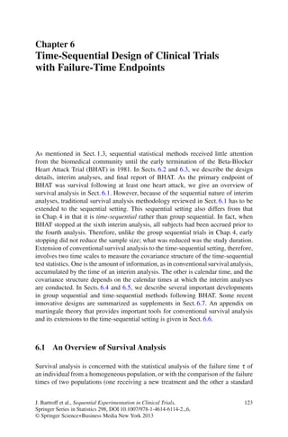
![124 6 Time-Sequential Design of Clinical Trials with Failure-Time Endpoints
one or placebo), or with regression analysis of τ on covariates. An important feature
of survival analysis is that some subjects in the study may not fail during the
observation period or may have withdrawn from the study during the period. Thus,
the data from these subjects are right censored. This makes the statistical analysis
much more complicated than the case in which all failure times in the sample
are fully observable. The time-sequential setting further increases the complexity
considerably. A theoretical tool to simplify the analytic calculations is martingale
theory. The overview takes advantage of this tool whose background is given in
Sect. 6.6.
6.1.1 Nelson–Aalen and Kaplan–Meier Estimators
Let τ1 , . . . , τn be n independent failure times with common distribution F. If F is
absolutely continuous with density function f , then
λ (t) = lim P(t ≤ τi < t + h | τ ≥ t)/h = f (t)/(1 − F(t))
h→0+
is called the hazard (or intensity) function; its integral Λ (t) = 0 λ (s)ds is called
t
the cumulative hazard function. More generally, the cumulative hazard function is
defined by
t dF(s)
Λ (t) = ,
0 1 − F(s−)
where F(s−) = limt→s− F(t).
The τi are subject to right censoring, which may be due to withdrawal or
the restricted length of the survival study. Thus, there are censoring variables ci ,
representing the time in the study during the observation period. The observations,
therefore, are (Ti , δi ), i = 1, · · · , n, where Ti = min(τi , ci ) and δi = I{τi ≤ci } is the
censoring indicator that indicates whether Ti is an actual failure time or is censored.
Subject i is “at risk” at time s if Ti ≥ s (i.e., has not failed and not withdrawn prior
to s). Let
n n
Y (s) = ∑ I{Ti ≥s} , N(s) = ∑ I{Ti ≤s, δi =1} . (6.1)
i=1 i=1
Note that Y (s) is the risk set size and Δ N(s) = N(s) − N(s−) is the number of
observed deaths at time s. The Nelson–Aalen estimator of the cumulative hazard
function Λ (t) is
Δ N(s) t I
{Y (s)>0}
Λ (t) = ∑
ˆ = dN(s), (6.2)
s≤t Y (s) 0 Y (s)
where we use the convention 0/0 = 0. It is shown in Sect. 6.6 that
t
U(s)[dN(s) − Y (s)d Λ (s)], t ≥ 0 is a martingale, (6.3)
0](data:image/gif;base64,R0lGODlhAQABAIAAAAAAAP///yH5BAEAAAAALAAAAAABAAEAAAIBRAA7)