2. 2 1 Piecewise Polynomial Approximation in 1D
To prove this, let us assume that the values ˛0 D v.x0 / and ˛1 D v.x1 / are given.
Inserting x D x0 and x D x1 into v.x/ D c0 C c1 x we obtain the linear system
Ä Ä Ä
1 x0 c0 ˛
D 0 (1.2)
1 x1 c1 ˛1
for ci , i D 1; 2.
Computing the determinant of the system matrix we find that it equals x1 x0 ,
which also happens to be the length of the interval I . Hence, the determinant is
positive, and therefore there exist a unique solution to (1.2) for any right hand side
vector. Moreover, as a consequence, there is exactly one function v in P1 .I /, which
has the values ˛0 and ˛1 at x0 and x1 , respectively. In the following we shall refer
to the points x0 and x1 as the nodes.
We remark that the system matrix above is called a Vandermonde matrix.
Knowing that we can completely specify any function in P1 .I / by its node values
˛0 and ˛1 we now introduce a new basis f 0 ; 1 g for P1 .I /. This new basis is called
a nodal basis, and is defined by
(
1; if i D j
j .xi / D ; i; j D 0; 1 (1.3)
0; if i ¤ j
From this definition we see that each basis function j , j D 0; 1, is a linear function,
which takes on the value 1 at node xj , and 0 at the other node.
The reason for introducing the nodal basis is that it allows us to express any
function v in P1 .I / as a linear combination of 0 and 1 with ˛0 and ˛1 as
coefficients. Indeed, we have
v.x/ D ˛0 0 .x/ C ˛1 1 .x/ (1.4)
This is in contrast to the monomial basis, which given the node values requires
inversion of the Vandermonde matrix to determine the corresponding coefficients c0
and c1 .
The nodal basis functions take the following explicit form on I
x1 x x x0
0 .x/ D ; 1 .x/ D (1.5)
x1 x0 x1 x0
This follows directly from the definition (1.3), or by solving the linear system (1.2)
with Œ1; 0T and Œ0; 1T as right hand sides.
1.1.2 The Space of Continuous Piecewise Linear Polynomials
A natural extension of linear functions is piecewise linear functions. In constructing
a piecewise linear function, v, the basic idea is to first subdivide the domain of v
into smaller subintervals. On each subinterval v is simply given by a linear function.
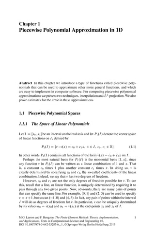
3. 1.1 Piecewise Polynomial Spaces 3
Fig. 1.1 A continuous
piecewise linear function v
v(x)
x
x0 x1 x2 x3 x4 x5
Continuity of v between adjacent subintervals is enforced by placing the degrees of
freedom at the start- and end-points of the subintervals. We shall now formalize this
more mathematically stringent.
Let I D Œ0; L be an interval and let the n C 1 node points fxi gnD0 define a
i
partition
I W 0 D x0 < x1 < x2 < : : : < xn 1 < xn D L (1.6)
of I into n subintervals Ii D Œxi 1 ; xi , i D 1; 2 : : : ; n, of length hi D xi xi 1 .
We refer to the partition I as to a mesh.
On the mesh I we define the space Vh of continuous piecewise linear functions
by
Vh D fv W v 2 C 0 .I /; vjIi 2 P1 .Ii /g (1.7)
where C 0 .I / denotes the space of continuous functions on I , and P1 .Ii / denotes
the space of linear functions on Ii . Thus, by construction, the functions in Vh are
linear on each subinterval Ii , and continuous on the whole interval I . An example
of such a function is shown in Fig. 1.1
It should be intuitively clear that any function v in Vh is uniquely determined by
its nodal values
fv.xi /gnD0
i (1.8)
and, conversely, that for any set of given nodal values f˛i gnD0 there exist a function v
i
in Vh with these nodal values. Motivated by this observation we let the nodal values
define our degrees of freedom and introduce a basis f'j gn D0 for Vh associated with
j
the nodes and such that
(
1; if i D j
'j .xi / D ; i; j D 0; 1; : : : ; n (1.9)
0; if i ¤ j
The resulting basis functions are depicted in Fig. 1.2.
Because of their shape the basis functions 'i are often called hat functions. Each
hat function is continuous, piecewise linear, and takes a unit value at its own node xi ,
while being zero at all other nodes. Consequently, 'i is only non-zero on the two
4. 4 1 Piecewise Polynomial Approximation in 1D
Fig. 1.2 A typical hat
'0 'i
function 'i on a mesh. Also
1
shown is the “half hat” '0
x
x0 x1 xi−1 xi xi+1 xn
intervals Ii and Ii C1 containing node xi . Indeed, we say that the support of 'i is
Ii [Ii C1 . The exception is the two “half hats” '0 and 'n at the leftmost and rightmost
nodes a D x0 and xn D b with support only on one interval.
By construction, any function v in Vh can be written as a linear combination
of hat functions f'i gnD0 and corresponding coefficients f˛i gnD0 with ˛i D v.xi /,
i i
i D 0; 1; : : : ; n, the nodal values of v. That is,
X
n
v.x/ D ˛i 'i .x/ (1.10)
i D0
The explicit expressions for the hat functions are given by
8
ˆ.x xi 1 /= hi ;
ˆ if x 2 Ii
<
'i D .xi C1 x/= hi C1 ; if x 2 Ii C1 (1.11)
ˆ
ˆ
:0; otherwise
1.2 Interpolation
We shall now use the function spaces P1 .I / and Vh to construct approximations,
one from each space, to a given function f . The method we are going to use is
very simple and only requires the evaluation of f at the node points. It is called
interpolation.
1.2.1 Linear Interpolation
As before, we start on a single interval I D Œx0 ; x1 . Given a continuous function f
on I , we define the linear interpolant f 2 P1 .I / to f by
f .x/ D f .x0 /'0 C f .x1 /'1 (1.12)
We observe that interpolant approximates f in the sense that the values of f and
f are the same at the nodes x0 and x1 (i.e., f .x0 / D f .x0 / and f .x1 / D f .x1 /).
5. 1.2 Interpolation 5
Fig. 1.3 A function f and its
linear interpolant f
p f(x)
f(x)
x
x0 x1
In Fig. 1.3 we show a function f and its linear interpolant f .
Unless f is linear, f will only approximate f , and it is therefore of interest to
measure the difference f f , which is called the interpolation error. To this end,
we need a norm. Now, there are many norms and it is not easy to know which is the
best. For instance, should we measure the interpolation error in the infinity norm,
defined by
kvk1 D max jv.x/j (1.13)
x2I
2
or the L .I /-norm defined, for any square integrable function v on I , by
ÂZ Ã1=2
kvkL2 .I / D v2 dx (1.14)
I
We shall use the latter norm, since it captures the average size of a function,
whereas the former only captures the pointwise maximum.
In this context we recall that the L2 .I /-norm, or any norm for that matter, obeys
the Triangle inequality
kv C wkL2 .I / Ä kvkL2 .I / C kwkL2 .I / (1.15)
as well as the Cauchy-Schwarz inequality
Z
vw dx Ä kvkL2 .I / kwkL2 .I / (1.16)
I
for any two functions v and w in L2 .I /.
Then, using the L2 -norm to measure the interpolation error, we have the
following results.
Proposition 1.1. The interpolant f satisfies the estimates
kf f kL2 .I / Ä C h2 kf 00 kL2 .I / (1.17)
k.f f /0 kL2 .I / Ä C hkf 00 kL2 .I / (1.18)
where C is a constant, and h D x1 x0 .
6. 6 1 Piecewise Polynomial Approximation in 1D
Proof. Let e D f f denote the interpolation error.
From the fundamental theorem of calculus we have, for any point y in I ,
Z y
e.y/ D e.x0 / C e 0 dx (1.19)
x0
where e.x0 / D f .x0 / f .x0 / D 0 due to the definition of f .
Now, using the Cauchy-Schwarz inequality we have
Z y
e.y/ D e 0 dx (1.20)
x0
Z y
Ä je 0 j dx (1.21)
x0
Z
Ä 1 je 0 j dx (1.22)
I
ÂZ Ã1=2 ÂZ Ã1=2
Ä 12 dx e 02 dx (1.23)
I I
ÂZ Ã1=2
02
Dh 1=2
e dx (1.24)
I
or, upon squaring both sides,
Z
e.y/2 Ä h e 02 dx D hke 0 k2 2 .I /
L (1.25)
I
Integrating this inequality over I we further have
Z Z
kek2 2 .I / D
L e.y/2 dy Ä hke 0 k2 2 .I / dy D h2 ke 0 k2 2 .I /
L L (1.26)
I I
since the integrand to the right of the inequality is independent of y. Thus, we have
kekL2 .I / Ä hke 0 kL2 .I / (1.27)
With a similar, but slightly different argument, we also have
ke 0 kL2 .I / Ä hke 00 kL2 .I / (1.28)
Hence, we conclude that
kekL2 .I / Ä hke 0 kL2 .I / Ä h2 ke 00 kL2 .I / (1.29)
7. 1.2 Interpolation 7
Fig. 1.4 The function f(x)
f .x/ D 2x sin.2 x/ C 3 and
its continuous piecewise
linear interpolant f .x/ on a
uniform mesh of I D Œ0; 1 3
with six nodes xi ,
i D 0; 1; : : : ; 5
p f(x)
2
x
0 = x0 x1 x2 x3 x4 x5 = 1
from which the first inequality of the proposition follows by noting that since f
is linear e 00 D f 00 . The second inequality of the proposition follows similarly
from (1.26)
The difference in argument between deriving (1.27) and (1.28) has to do with the
fact that we can not simply replace e with e 0 in (1.19), since e 0 .x0 / ¤ 0. However,
noting that e.x0 / D e.x1 / D 0, there exist by Rolle’s theorem a point x in I such
N
that e 0 .x/ D 0, which means that
N
Z y Z y
0 0 00
e .y/ D e .x/ C
N e dx D e 00 dx (1.30)
N
x N
x
Starting instead from this and proceeding as shown above (1.28) follows. t
u
Examining the proof of Proposition 1.1 we note that the constant C equals unity
and could equally well be left out. We have, however, chosen to retain this constant,
since the estimates generalize to higher spatial dimensions, where C is not unity.
The important thing to understand is how the interpolation error depends on the
interpolated function f , and the size of the interval h.
1.2.2 Continuous Piecewise Linear Interpolation
It is straight forward to extend the concept of linear interpolation on a single interval
to continuous piecewise linear interpolation on a mesh. Indeed, given a continuous
function f on the interval I D Œ0; L, we define its continuous piecewise linear
interpolant f 2 Vh on a mesh I of I by
X
n
f .x/ D f .xi /'i .x/ (1.31)
i D1
Figure 1.4 shows the continuous piecewise linear interpolant f .x/ to f .x/ D
2x sin.2 x/ C 3 on a uniform mesh of I D Œ0; 1 with 6 nodes.
Regarding the interpolation error f f we have the following results.
8. 8 1 Piecewise Polynomial Approximation in 1D
Proposition 1.2. The interpolant f satisfies the estimates
X
n
kf f k2 2 .I / Ä C
L h4 kf 00 k2 2 .Ii /
i L (1.32)
i D1
X
n
k.f f /0 k2 2 .I / Ä C
L h2 kf 00 k2 2 .Ii /
i L (1.33)
i D1
Proof. Using the Triangle inequality and Proposition 1.1, we have
X
n
kf f k2 2 .I / D
L kf f k2 2 .Ii /
L (1.34)
i D1
X
n
Ä C h4 kf 00 k2 2 .Ii /
i L (1.35)
i D1
which proves the first estimate. The second follows similarly. t
u
Proposition 1.2 says that the interpolation error vanish as the mesh size hi tends to
zero. This is natural, since we expect the interpolant f to be a better approximation
to f where ever the mesh is fine. The proposition also says that if the second
derivative f 00 of f is large then the interpolation error is also large. This is also
natural, since if the graph of f bends a lot (i.e., if f 00 is large) then f is hard to
approximate using a piecewise linear function.
1.3 L2 -Projection
Interpolation is a simple way of approximating a continuous function, but there
are, of course, other ways. In this section we shall study so-called orthogonal-, or
L2 -projection. L2 -projection gives a so to speak good on average approximation,
as opposed to interpolation, which is exact at the nodes. Moreover, in contrast to
interpolation, L2 -projection does not require the function we seek to approximate
to be continuous, or have well-defined node values.
1.3.1 Definition
Given a function f 2 L2 .I / the L2 -projection Ph f 2 Vh of f is defined by
Z
.f Ph f /v dx D 0; 8v 2 Vh (1.36)
I
9. 1.3 L2 -Projection 9
f − Ph f
f
v
Ph f
Vh
Fig. 1.5 Illustration of the function f and its L2 -projection Ph f on the space Vh
Fig. 1.6 The function
f .x/ D 2x sin.2 x/ C 3 and
its L2 -projection Ph f on a
uniform mesh of I D Œ0; 1 3
with six nodes, xi ,
i D 1; 2; : : : ; 6
2
f(x)
1
Ph f(x)
x
0 = x0 x1 x2 x3 x4 x5 = 1
In analogy with projection onto subspaces of Rn , (1.34) defines a projection of f
onto Vh , since the difference f Ph f is required to be orthogonal to all functions
v in Vh . This is illustrated in Fig. 1.5.
As we shall see later on, Ph f is the minimizer of minv2Vh kf vkL2 .I / , and
therefore we say that it approximates f in a least squares sense. In fact, Ph f is the
best approximation to f when measuring the error f Ph f in the L2 -norm.
In Fig. 1.6 we show the L2 -projection of f .x/ D 2x sin.2 x/ C 3 computed on
the same mesh as was used for showing the continuous piecewise linear interpolant
f in Fig. 1.4. It is instructive to compare these two approximations because it
highlights their different characteristics. The interpolant f approximates f exactly
at the nodes, while the L2 -projection Ph f approximates f on average. In doing
so, it is common for Ph f to over and under shoot local maxima and minima of
f , respectively. Also, both the interpolant and the L2 -projection have difficulty
with approximating rapidly oscillating or discontinuous functions unless the node
positions are adjusted appropriately.
10. 10 1 Piecewise Polynomial Approximation in 1D
1.3.2 Derivation of a Linear System of Equations
In order to actually compute the L2 -projection Ph f , we first note that the defini-
tion (1.36) is equivalent to
Z
.f Ph f /'i dx D 0; i D 0; 1; : : : ; n (1.37)
I
where 'i , i D 0; 1; : : : ; n, are the hat functions. This is a consequence of the fact
that if (1.36) is satisfied for v anyone of the hat functions, then it is also satisfied
for v a linear combination of hat functions. Conversely, since any function v in Vh is
precisely such a linear combination of hat functions, (1.37) implies (1.36).
Then, since Ph f belongs to Vh it can be written as the linear combination
X
n
Ph f D j 'j (1.38)
j D0
where j , j D 0; 1; : : : ; n, are n C 1 unknown coefficients to be determined.
Inserting the ansatz (1.38) into (1.37) we get
0 1
Z Z X
n
f 'i dx D @ j 'j A 'i dx (1.39)
I I j D0
X
n Z
D j 'j 'i dx; i D 0; 1; : : : ; n (1.40)
j D0 I
Further, introducing the notation
Z
Mij D 'j 'i dx; i; j D 0; 1; : : : ; n (1.41)
I
Z
bi D f 'i dx; i D 0; 1; : : : ; n (1.42)
I
we have
X
n
bi D Mij j; i D 0; 1; : : : ; n (1.43)
j D0
which is an .n C 1/ .n C 1/ linear system for the n C 1 unknown coefficients j,
j D 0; 1; : : : ; n. In matrix form, we write this
M Db (1.44)
11. 1.3 L2 -Projection 11
where the entries of the .n C 1/ .n C 1/ matrix M and the .n C 1/ 1 vector b
are defined by (1.41) and (1.42), respectively.
We, thus, conclude that the coefficients j , j D 0; 1; : : : ; n in the ansatz (1.38)
satisfy a square linear system, which must be solved in order to obtain the L2 -
projection Ph f .
For historical reasons we refer to M as the mass matrix and to b as the load
vector.
1.3.3 Basic Algorithm to Compute the L2 -Projection
The following algorithm summarizes the basic steps for computing the L2 -
projection Ph f :
Algorithm 1 Basic algorithm to compute the L2 -projection
1: Create a mesh with n elements on the interval I and define the corresponding space of
continuous piecewise linear functions Vh .
2: Compute the .n C 1/ .n C 1/ matrix M and the .n C 1/ 1 vector b, with entries
Z Z
Mij D 'j 'i dx; bi D f 'i dx (1.45)
I I
3: Solve the linear system
M Db (1.46)
4: Set
X
n
Ph f D j 'j (1.47)
j D0
1.3.4 A Priori Error Estimate
Naturally, we are interested in knowing how good Ph f is at approximating f . In
particular, we wish to derive bounds for the error f Ph f . The next theorem gives
a key result for deriving such error estimates. It is a so-called a best approximation
result.
Theorem 1.1. The L2 -projection Ph f , defined by (1.36), satisfies the best approx-
imation result
kf Ph f kL2 .I / Ä kf vkL2 .I / ; 8v 2 Vh (1.48)
Proof. Using the definition of the L2 -norm and writing f Ph f D f vCv Ph f ,
with v an arbitrary function in Vh , we have
12. 12 1 Piecewise Polynomial Approximation in 1D
Z
kf Ph f k2 2 .I / D
L .f Ph f /.f vCv Ph f / dx (1.49)
I
Z Z
D .f Ph f /.f v/ dx C .f Ph f /.v Ph f / dx
I I
(1.50)
Z
D .f Ph f /.f v/ dx (1.51)
I
Ä kf Ph f kL2 .I / kf vkL2 .I / (1.52)
where we used the definition of the L2 -projection to conclude that
Z
.f Ph f /.v Ph f / dx D 0 (1.53)
I
since v Ph f 2 Vh . Dividing by kf Ph f kL2 .I / concludes the proof. t
u
This shows that Ph f is the closest of all functions in Vh to f when measuring in
the L2 -norm. Hence, the name best approximation result.
We can use best approximation result together with interpolation estimates to
study how the error f Ph f depends on the mesh size. In doing so, we have the
following basic so-called a priori error estimate.
Theorem 1.2. The L2 -projection Ph f satisfies the estimate
X
n
kf Ph f k2 2 .I / Ä C
L h4 kf 00 k2 2 .Ii /
i L (1.54)
i D1
Proof. Starting from the best approximation result, choosing v D f the interpolant
of f , and using the interpolation error estimate of Proposition 1.1, we have
kf Ph f k2 2 .I / Ä kf
L f k2 2 .I /
L (1.55)
X
n
Ä kf f k2 2 .Ii /
L (1.56)
i D1
X
n
Ä C h4 kf 00 k2 2 .Ii /
i L (1.57)
i D1
which proves the estimate. t
u
Defining h D max1Äi Än hi we conclude that
kf Ph f kL2 .I / Ä C h2 kf 00 kL2 .I / (1.58)
Thus, the L2 -error kf Ph f kL2 .I / tends to zero as the maximum mesh size h tends
to zero.
13. 1.4 Quadrature 13
1.4 Quadrature
To compute the L2 -projection we need to compute the mass matrix M whose entries
are integrals involving products of hat functions. One way of doing this is to use
quadrature, or, numerical integration. To this end, f be a continuous function on
the interval I D Œx0 ; x1 , and consider the problem of evaluating, approximately,
the integral
Z
J D f .x/ dx (1.59)
I
A quadrature rule is a formula that is used to compute integrals approximately.
It it usually derived by first interpolating the integrand f by a polynomial and then
integrating the interpolant. Depending on the degree of the interpolating polynomial
one obtains quadrature rules of different computational complexity and accuracy.
Evaluating a quadrature rule generally involves summing values of the integrand f
at a set of carefully selected quadrature points within the interval I times the interval
length h D x1 x0 . We shall next describe three classical quadrature rules called the
Mid-point rule, the Trapezoidal rule, and Simpson’s formula, which corresponds to
using polynomial interpolation of degree 0, 1, and 2 on f , respectively.
1.4.1 The Mid-Point Rule
Interpolating f with the constant f .m/, where m D .x0 C x1 /=2 is the mid-point
of I , we get
J f .m/h (1.60)
which is the Mid-point rule. Geometrically this means that we approximate the area
under the integrand f with the area of the square f .m/h, see Fig. 1.7. The Mid-
point rule integrates linear polynomials exactly.
1.4.2 The Trapezoidal Rule
Continuing, interpolating f with the line passing through the points .x0 ; f .x0 // and
.x1 ; f .x1 // we get
f .x0 / C f .x1 /
J h (1.61)
2
which is the Trapezoidal rule. Geometrically this means that we approximate the
area under f with the area under the trapezoidal with the four corner points .x0 ; 0/,
14. 14 1 Piecewise Polynomial Approximation in 1D
Fig. 1.7 The area of the
shaded square approximates
R f(x)
J D I f .x/ dx
x
x0 m x1
Fig. 1.8 The area of the
shaded trapezoidal
f(x)
approximates
R
J D I f .x/ dx
x
x0 x1
.x0 ; f .x0 //, .x1 ; 0/, and .x1 ; f .x1 //, see Fig. 1.8. The Trapezoidal rule is also exact
for linear polynomials.
1.4.3 Simpson’s Formula
This rule corresponds to a quadratic interpolant using the end-points and the mid-
point of the interval I as nodes. To simplify things a bit let I D Œ0; l be the interval
of integration and let g.x/ D c0 Cc1 x Cc2 x 2 be the interpolant. Since g interpolates
l l
f at the points .0; f .0//, . 2 ; f . 2 //, and .l; f .l// (i.e., its graph passes trough these
points) their coordinates must satisfy the equation for g. This yields the following
linear system for c0 , c1 , and c2 .
2 32 3 2 3
0 0 1 c0 f .0/
4 1 l 2 1 l 15 4c1 5 D 4f . l /5 (1.62)
4 2 2
l2 l 1 c2 f .l/
Solving this one readily finds
c0 D 2.f .0/ 2f . 2 / Cf .l//= l 2 ; c1 D
l
.3f .0/ 4f . 2 / Cf .l//= l; c2 D f .0/
l
(1.63)
Now, integrating g from 0 to l one eventually ends up with
15. 1.5 Computer Implementation 15
Z l f .0/ C 4f . 1 l/ C f .l/
g.x/ dx D 2
l (1.64)
0 6
which is Simpson’s formula.
On the interval I D Œx0 ; x1 Simpson’s formula takes the form
f .x0 / C 4f .m/ C f .x1 /
J h (1.65)
6
with m D 1 .x0 C x1 / and h D x1 x0 .
2
Simpson’s formula is exact for third order polynomials.
1.5 Computer Implementation
1.5.1 Assembly of the Mass Matrix
Having studied various quadrature rules, let us now go through the nitty gritty details
of how to assembleRthe mass matrix M and load vector b. We begin by calculating
the entries Mij D I 'i 'j dx of the mass matrix. Because each hat 'i is a linear
polynomial the product of two hats is a quadratic polynomial. Thus, Simpson’s
formula can be used to integrate Mij exactly. In doing so, since the hats 'i and
'j lack common support for ji j j > 1 only Mi i , Mi i C1 , and Mi C1i need to be
calculated. All other matrix entries are zero by default. This is clearly seen from
Fig. 1.9 showing two neighbouring hat functions and their support. This leads to the
observation that the mass matrix M is tridiagonal.
Starting with the diagonal entries Mi i and using Simpson’s formula we have
Z
Mi i D 'i2 dx (1.66)
I
Z xi Z xi C1
D 'i2 dx C 'i2 dx (1.67)
xi 1 xi
0 C 4 . 1 /2 C 1 1 C 4 . 1 /2 C 0
D 2
hi C 2
hi C1 (1.68)
6 6
hi hi C1
D C ; i D 1; 2; : : : ; n 1 (1.69)
3 3
where xi xi 1 D hi and xi C1 xi D hi C1 . The first and last diagonal entry are
M00 D h1 =3 and Mnn D hn =3, respectively, since the hat functions '0 and 'n are
only half.
Continuing with the subdiagonal entries Mi C1 i , still using Simpson’s formula,
we have
16. 16 1 Piecewise Polynomial Approximation in 1D
Fig. 1.9 Illustration of the
'i−1 'i
hat functions 'i 1 and 'i and
1
their support
x
xi−2 xi−1 xi xi+1
Z
Mi C1 i D 'i 'i C1 dx (1.70)
I
Z xi C1
D 'i 'i C1 dx (1.71)
xi
1 0 C 4 . 1 /2 C 0 1
D 2
hi C1 (1.72)
6
hi C1
D ; i D 0; 1; : : : ; n (1.73)
6
A similar calculation shows that the superdiagonal entries are Mi i C1 D hi C1 =6.
Hence, the mass matrix takes the form
2h h
3
1 1
3 6
6 h1 h1
C h2 h2 7
66 7
6 3 3 6
7
6 h2 h2
C h3 h3
7
M D6 7
6 3 3 6
6 :: :: :: 7 (1.74)
6 : : : 7
6 hn 7
4 hn
6
1 hn
3
1
C hn
3 6
5
hn hn
6 3
From (1.74) it is evident that the global mass matrix M can be written as a sum
of n simple matrices, viz.,
2h 3 2 3 2 3
1 h1
3 6
6 h1 h1 7 6 h2 h2 7 6 7
66 3 7 6 7 6 7
6 7 6 3 6
h2 h2 7 6 7
6 7 6 7 6 7
M D6 7C6 6 3 7 C ::: C 6 7 (1.75)
6 7 6 7 6 7
6 7 6 7 6 hn 7
4 5 4 5 4 hn
3 6
5
hn hn
6 3
D M I1 C M I2 C : : : C M In (1.76)
Each matrix M Ii , i D 1; 2 : : : ; n, is obtained by restricting integration to one
subinterval, or element, Ii and is therefore called a global element mass matrix.
In practice, however, these matrices are never formed, since it suffice to compute
their 2 2 blocks of non-zero entries. From the sum (1.75) we see that on each
17. 1.5 Computer Implementation 17
element I this small block takes the form
Ä
1 21
M D I
h (1.77)
6 12
where h is the length of I . We refer to M I as the local element mass matrix.
The summation of the element mass matrices into the global mass matrix is
called assembling. The assembly process lies at the very heart of finite element
programming because it allows the forming of the mass matrix through the use of a
single loop over the elements. It also generalizes to higher dimensions.
The following algorithm summarizes how to assemble the mass matrix M :
Algorithm 2 Assembly of the mass matrix
1: Allocate memory for the .n C 1/ .n C 1/ matrix M and initialize all matrix entries to zero.
2: for i D 1; 2; : : : ; n do
3: Compute the 2 2 local element mass matrix M I given by
Ä
1 21
M D
I
h (1.78)
6 12
where h is the length of element Ii .
I
4: Add M11 to Mi i
I
5: Add M12 to Mi iC1
I
6: Add M21 to MiC1i
I
7: Add M22 to MiC1iC1
8: end for
The following MATLAB routine assembles the mass matrix.
function M = MassAssembler1D(x)
n = length(x)-1; % number of subintervals
M = zeros(n+1,n+1); % allocate mass matrix
for i = 1:n % loop over subintervals
h = x(i+1) - x(i); % interval length
M(i,i) = M(i,i) + h/3; % add h/3 to M(i,i)
M(i,i+1) = M(i,i+1) + h/6;
M(i+1,i) = M(i+1,i) + h/6;
M(i+1,i+1) = M(i+1,i+1) + h/3;
end
Input to this routine is a vector x holding the node coordinates. Output is the global
mass matrix.
18. 18 1 Piecewise Polynomial Approximation in 1D
1.5.2 Assembly of the Load Vector
R
We next calculate the load vector b. Because the entries bi D i f 'i dx depend on
the function f , we can not generally expect to calculate them exactly. However, we
can approximate entry bi using a quadrature rule. Using the Trapezoidal rule, for
instance, we have
Z
bi D f 'i dx (1.79)
I
Z xi C1
D f 'i dx (1.80)
xi 1
Z xi Z xi C1
D f 'i dx C f 'i dx (1.81)
xi 1 xi
.f .xi 1 /'i .xi 1 / C f .xi /'i .xi //hi =2 (1.82)
C .f .xi /'i .xi / C f .xi C1 /'i .xi C1 //hi C1 =2 (1.83)
D .0 C f .xi //hi =2 C .f .xi / C 0/hi C1 =2 (1.84)
D f .xi /.hi C hi C1 /=2 (1.85)
The approximate load vector then takes the form
2 3
f .x0 /h1 =2
6 7
f .x1 /.h1 C h2 /=2
6 7
6 7
6 f .x2 /.h2 C h3 /=2
7
bD6
6 :7
7 (1.86)
6 :
:7
6 7
4f .xn 1 /.hn 1 C hn /=25
f .xn /hn =2
Splitting b into a sum over the elements yields the n global element load vectors
b Ii
2 3 2 3 2 3
f .x0 /
6f .x /7 6f .x /7 6 7
6 1 7 6 1 7 6 7
6 7 6 7 6 7
bD6 7 h1 =2 C 6f .x2 /7 h2 =2 C : : : C 6 7 hn =2 (1.87)
6 7 6 7 6 7
4 5 4 5 4f .xn 1 /5
f .xn /
D b I1 C b I2 C : : : C b In : (1.88)
19. 1.5 Computer Implementation 19
Each vector b Ii , i D 1; 2; : : : ; n, is obtained by restricting integration to element Ii .
The assembly of the load vector b is very similar to that of the mass matrix as the
following algorithm shows:
Algorithm 3 Assembly of the load vector
1: Allocate memory for the .n C 1/ 1 vector b and initialize all vector entries to zero.
2: for i D 1; 2; : : : ; n do
3: Compute the 2 1 local element load vector b I given by
Ä
1 f .xi 1 /
bI D h (1.89)
2 f .xi /
where h is the length of element Ii .
I
4: Add b1 to bi 1
I
5: Add b2 to bi
6: end for
A MATLAB routine for assembling the load vector is listed below.
function b = LoadAssembler1D(x,f)
n = length(x)-1;
b = zeros(n+1,1);
for i = 1:n
h = x(i+1) - x(i);
b(i) = b(i) + f(x(i))*h/2;
b(i+1) = b(i+1) + f(x(i+1))*h/2;
end
Here, f is assumed to be a separate routine specifying the function f . This needs
perhaps a little bit of explanation. MATLAB has a something called function
handles, which provide a way of passing a routine as argument to another routine.
For example, suppose we have written a routine called Foo1 to specify the function
f .x/ D x sin.x/
function y = Foo1(x)
y=x.*sin(x)
To assemble the corresponding load vector, we type
b = LoadAssembler1D(x,@Foo1)
This passes the routine Foo1 as argument to LoadAssembler1D and allows it to be
evaluated inside the assembler. The at sign @ creates the function handle. Indeed,
function handles provide means for writing flexible and reusable code.
In this context we mention that if Foo1 is a small routine, then it can be inlined
and called, viz.,
Foo1 = inline(’x.*sin(x)’,’x’)
b = LoadAssembler1D(x,Foo1)
20. 20 1 Piecewise Polynomial Approximation in 1D
Note that there is no at sign in the call to the load vector assembler.
Putting it all together we get the following main routine for computing L2 -
projections.
function L2Projector1D()
n = 5; % number of subintervals
h = 1/n; % mesh size
x = 0:h:1; % mesh
M = MassAssembler1D(x); % assemble mass
b = LoadAssembler1D(x,@Foo1); % assemble load
Pf = Mb; % solve linear system
plot(x,Pf) % plot L^2 projection
1.6 Problems
Exercise 1.1. Let I D Œx0 ; x1 . Verify by direct calculation that the basis functions
x1 x x x0
0 .x/ D ; 1 .x/ D
x1 x0 x1 x0
for P1 .I / satisfies 0 .x/ C 1 .x/ D 1 and x0 0 .x/ C x1 1 .x/ D x. Give
a geometrical interpretation by drawing 0 .x/, 1 .x/, 0 .x/ C 1 .x/, x0 0 .x/,
x1 1 .x/ and x0 0 .x/ C x1 1 .x/.
Exercise 1.2. Let 0 D x0 < x1 < x2 < x3 D 1, where x1 D 1=6 and x2 D 1=2, be
a partition of the interval I D Œ0; 1 into three subintervals, and let Vh be the space
of continuous piecewise linear functions on this partition.
(a) Determine analytical expressions for the hat function '1 .x/ and draw it.
(b) Draw the function v.x/ D '0 .x/ C '2 .x/ C 2'3 .x/ and its derivative v0 .x/.
(c) Draw the piecewise constant mesh function h.x/ D hi on each subinterval Ii .
(d) What is the dimension of Vh ?
Exercise 1.3. Determine the linear interpolant f 2 P1 .I / on the single interval
I D Œ0; 1 to the following functions f .
(a) f .x/ D x 2 .
(b) f .x/ D 3 sin.2 x/.
Make plots of f and f in the same figure.
Exercise 1.4. Let Vh be the space of all continuous piecewise linears on a uniform
mesh with four nodes of I D Œ0; 1. Draw the interpolant f 2 Vh to the following
functions f .
(a) f .x/ D x 2 C 1.
(b) f .x/ D cos. x/.
21. 1.6 Problems 21
Can you think of a better partition of I assuming we are restricted to three
subintervals?
Exercise 1.5. Calculate kf k1 with f D x.x 1=2/.x 1=3/ on the interval
I D Œ0; 1.
Exercise 1.6. Let I D Œ0; 1 and f .x/ D x 2 for x 2 I .
R
(a) Calculate R I f dx analytically.
(b) Compute RI f dx using the Mid-point rule.
(c) Compute I f dx using the Trapezoidal rule.
(d) Compute the quadrature errors in (b) and (c).
Exercise 1.7. Let I D Œ0; 1 and f .x/ D x 4 for x 2 I .
R
(a) Calculate R I f dx analytically.
(b) Compute I f dx using Simpson’s formula on the single interval I .
R
(c) Divide I into two equal subintervals and compute I f dx using Simpson’s
formula on each subinterval.
(d) Compute the quadrature errors in (b) and (c). By what factor has the error
decreased?
Exercise 1.8. Let I D Œ0; 1 and let f .x/ D x 2 for x 2 I .
(a) Let Vh be the space P1 .I / of linear functions on I . Compute the L2 -projection
Ph f 2 Vh of f .
(b) Divide I into two subintervals of equal length and let Vh be the corresponding
space Vh of continuous piecewise linear functions. Compute the L2 -projection
Ph f 2 Vh of f .
(c) Plot your results and compare with the nodal interpolant f .
R
Exercise 1.9. Show that ˝ .f
R Ph f /v dx D 0 for all v 2 Vh , if and only if
˝ .f Ph f /'i dx D 0, for i D 0; 1; : : : ; n, where f'i gnD0 Vh is the usual basis
i
of hat functions.
R
Exercise 1.10. Let .f; g/ D I fg dx and kf k2 2 .I / D .f; f / denote the L2 -scalar
L
product and norm, respectively. Also, let I D Œ0; , f D x, g D cos.x/, and
h D 2 cos.3x/ for x 2 I .
(a) Calculate .f; g/.
(b) Calculate .g; h/. Are g and h orthogonal?
(c) Calculate kf kL2 .I / and kgkL2 .I / .
Exercise 1.11. Let V be a linear subspace of Rn with basis fv1 ; : : : ; vm g with
m < n. Let P x 2 V be the orthogonal projection of x 2 Rn onto the subspace V .
Derive a linear system of equations that determines P x. Note that your results are
analogous to the L2 -projection when the usual scalar product in Rn is replaced by
the scalar product in L2 .I /. Compare this method of computing the projection P x
to the method used for computing the projection of a three dimensional vector onto a
two dimensional subspace. What happens if the basis fv1 ; : : : ; vm g is L2 -orthogonal?
22. 22 1 Piecewise Polynomial Approximation in 1D
Exercise 1.12. Show that f1; x; .3x 2 1/=2g form a basis for the space of quadratic
polynomials P2 .I /, on I D Π1; 1. Then compute and draw the L2 -projections
Ph f 2 P2 .I / on I for the following two functions f .
(a) f .x/ D 1 C 2x.
(b) f .x/ D x 3 .
Exercise 1.13. Show that the hat function basis f'j gn D0 of Vh is almost orthogonal.
j
How can we see that it is almost orthogonal by looking at the non-zero elements
of the mass matrix? What can we say about the mass matrix if we had a fully
orthogonal basis?
Exercise 1.14. Modify L2Projector1D and compute the L2 -projection Ph f of
the following functions f .
(a) f .x/ D 1.
(b) f .x/ D x 3 .x 1/.1 2x/.
(c) f .x/ D arctan..x 0:5/= /, with D 0:1 and 0:01.
Use a uniform mesh I of the interval I D Œ0; 1 with n D 5, 25, and 100 subintervals.