4. Oscillation Summary Natural climate oscillations effect regional, hemispheric, and global weather and climate. Climate oscillation patterns are detectable in palaeoclimate proxies, And are thus not anthropogenic. The causes of climate oscillations are poorly understood; most have been defined only in the last 20 to 80 years. Climate oscillations are inter-related, e.g. ENSO and PDO. When in phase (e.g. warm phases of ENSO, PDO, AMO), global warming effect ~= warming of last century (0.6 O C). We are entering a cool PDO phase. PDO and AMO can explain much of recent Arctic sea ice melting and Alaskan glacier retreat. Super El Ninos occurred before industrialization, thus are not anthropogenic.
5. Global Mean Radiative Forcings in 2005 Adapted from IPCC 2007: WG1-AR4, page 32 0 -2 +2 +1 -1 Wm -2 Climate Oscillations are not Radiative Forcing (at least not directly) and thus do not show up on this IPCC balance sheet.
9. “ The current state of the science is that the effect [of the Urban Heat Island] on the global temperature record is small to negligible.” Real Climate “ This paper bends over backwards to argue for the retention of general warming…., despite finding evidence that landscape change (in this case, urbanization) alters long term trends.’’ Roger Pielke, Sr.
16. Land Use Summary It is likely that UHI imparts a warming bias to land-based temperature readings. Land management and land cover change are first order anthropogenic climate forcings. Land use changes are under valued by the IPCC (Pielke, Sr.), and thus the impact of GHG is over valued for the observed warming of the last century.
17. Global Mean Radiative Forcings in 2005 Adapted from IPCC 2007: WG1-AR4, page 32 Land Use Black Carbon on Snow Surface Albedo Direct Aerosol Cloud Albedo Linear Contrails 0 -2 +2 +1 -1 Wm -2 No volcanic aerosol effect is included The IPCC does not credit UHI heating
18. The Case for CAGW “ Extraordinary claims require extraordinary evidence,” Carl Sagan
19. Evidence that Carbon Global Warming 1. Temperature follows CO 2 levels in past. 2. Atmosphere shows characteristic heating pattern of adding GHG CO2, CH4
20. Not evidence of C AGW: Arctic ice disappearing Antarctic ice shelf breaks loose Glaciers retreating Coral reef bleaching Mt. Kilimanjaro losing snow Polar bear population changing A change in cyclones /hurricanes/typhoons Droughts Dry rivers
22. Well Mixed Green House Gases Records of changes in atmospheric composition over the past 1000 years. Ice core and firn data for several sites in Antarctica and Greenland are supplemented with the data from direct atmospheric samples over the past few decades. “ A Report of Working Group I of the Intergovernmental Panel on Climate Change”, United Nations, 2000
27. Wall Street Journal, Feb. 14, 2005 Mr. McIntyre thinks there are more errors [in the Mann hockeystick] but says his audit is limited because he still doesn't know the exact computer code Dr. Mann used to generate the graph. Dr. Mann refuses to release it. "Giving them the algorithm would be giving in to the intimidation tactics that these people are engaged in," he says. Dr. Mann says his busy schedule didn't permit him to respond to "every frivolous note" from nonscientists… Stephen McIntyre Michael Mann
28. Hearing of the Investigations Subcommittee of the House Energy and Commerce Committee, July, 2005 Michael Mann Stephen McIntyre It took an act of Congress to get the data released!
29. Bristlecone pine: Senior Citizens ~5,000 years old! www.flickr.com/photos/ Width and density of annual rings changes in temperature. Briffa, et al, 2008
30. Graybill, 1983 Holzmann in 2007 Mann Hockystick Depended on Graybill Bristlecone Pine Chronologies
31. Figure 14. Left and middle – two cross sections of Colorado bristlecones from Brunstein (2006); right – strip bark juniper from Karakorum, Pakistan used in Jan Esper chronology. Asymmetry prevent Accurate Coring
32.
33. The CENSORED File of PalaeoClimate Proxies “ We discovered that an undocumented directory at Mann’s FTP site entitled “CENSORED” contained calculations without bristlecones. Without the bristlecones, none of the PC series had a hockey stick shape.” James McIntyre, Climate Audit Temperature proxies from coral, ice cores, and historical records
34. Polar Urals tree line, advancing modern tree line in background, medieval tree line in foreground (Jan Esper) Other Studies Argued to Support Mann et al. Hockey Stick
39. It took 3 years and FIO to access archived data. S. McIntyre 27Sep09 Briffa 12 Yamal live tree cores CRU Archive substituting 34 Polar Ural recent live tree cores for Yamal cores MWP
40.
41. “ YAD06 is the most influential tree in the world. YAD06 does not always drink beer, but when it does, it drinks Dos Equis. Stay thirsty, my friends.” The Yamal Ten Steve McIntyre 30Sep09
42. Keith Briffa Professor at the Climatic Research Unit, University of East Anglia, Norwich, U.K. His specialism is dendroclimatology. A lead author of The Physical Science Basis, Chapter 6, Palaeoclimate, 2007 IPCC 4TAR
44. Glacier lines: 1922, 1856 A Pass in the Alps Modern Era Roman Times, 2000 years ago
45. Proxy Summary IPCC Hockey stick temperature curves are the result of Mannian manipulation, including the selective use of data. Bristlecone pine and other strip bark tree ring proxies are suspect thermometers. Few non-tree ring proxies produce a temperature hockey stick. A large body of evidence supports a Roman warm period, MWP, and Little Ice Age. Today’s temperatures are well within the 15 +/- 1 O C variation of this interglacial.
46. I’ve given up entirely on tree rings and am now focusing my efforts on petrified naked people. Find yourself a wad of those in some bog and you’ve got yourself a bonafied “warm period”.
73. GHCN 200 6 NOAA declares 2006 to be 5 th warmest
74. Warm Bias in Surface Temp. Record Surface minus Satellite Temperature = 0.20 O C/decade over land Land = 29% Global Surface IPCC Global projection of 0.20 O C/decade minus land bias 0.14 O C/decade corrected
89. “ This is much ado about nothing. The multiyear and multi-decadal changes in Global SST anomalies appear to reflect the ocean’s ability to integrate ENSO.” Bob Tisdale
92. Temperature Record Summary Ground-based measurements have a warm bias: UHI Effect, Urban bias over rural, Poor site condition, Night warm bias. Ocean Heat Content: Rose in last half of the last century, Has declined since 2003 despite increasing atmospheric CO 2 .
93. Temperature Record Summary SST measurements conflicting trends: Buoy data warming, Satellite data flat to slight cooling. Top-of-Atmosphere flux: ERBE: Hotter sea more heat radiated into space. Models: Hotter sea more heat retained by atmosphere. IPCC projections overstate warming.
96. " Human-made climate forcings, mainly greenhouse gases, heat the earth’s surface at a rate of about two watts per square meter—the equivalent of two tiny one-watt bulbs burning over every square meter of the planet " James Hanson, GISS 2 Wm -2 ~ +0.53 O C
97. 0.5 O C 0.22 O C with 40% cloud cover Requires humanity to completely take over all natural effects that were operating before the Industrial Revolution
98. 0.5 O C 0.22 O C with 40% cloud cover Requires humanity to completely take over all natural effects that were operating before the Industrial Revolution
99. Beer’s Law: Transmission of radiation is a logarithmic function of concentration. Logarithmic Response to GHG Concentration Delta T = alpha log (C/C 0 ) Svante Arrhenius, 1896
100.
101. Existing and Potential Anthropogenic CO 2 Greenhouse Effect Pre-Industrial CO 2 Greenhouse Effect
102. Graph by Bill Illis modified by Anthony Watts 25Oct09
103. Graph by Bill Illis modified by Anthony Watts 25Oct09
106. Climate Sensitivity (2 X CO 2 ) Without change in water vapor. CO 2 minus aerosols (no sun effect) H 2 O amplification 3.0 O C IPCC 1.4 O C Chylek 1.1 O C Schwartz, Clear sky (0.22 O C with 40% cloud cover) O.5 O C Lindzen O.46 O C Spencer O.37 O C Idso Saturated Greenhouse (more CO 2 less H 2 O) O O C Miskolczi
113. No Accelerated Warming RSS MSU Satellites 1979 to present The vertical axis is the global average temperature anomaly in degrees Celsius in the lower troposphere
116. 2X CO 2 = +1.2 O C IPCC Hypothesis 2X CO 2 = +3 to +6 O C Present GHG = +33 O C Moderation Hypothesis 2X CO 2 = +0.4 O C Qualitative illustration of green house warming.
121. Northern Hemisphere +0.28 O C/decade Southern Hemisphere +0.07 O C/decade Tropics +0.07 O C/decade What’s Warming the NH? CO 2 <4% Variation
122. CO 2 Warming Summary Hanson’s 2Wm -2 anthropogenic warming is indistinct from natural variability. GH effect is logarithmic: 2X CO 2 + 40 % clouds 0.22 O C. Earth annually adjusts to 4 O C temp. swings. Earth adjusts to El Nino heating. No predicted GHG tropical troposphere hot spot. Model presumption of constant RH is incorrect. RH (and SH at 400 mb) are declining. H 2 O amplification of CO 2 warming is not seen.
123. CO 2 Warming Summary Global temp. has not risen in last 10 years, despite increasing CO 2 . No accelerated warming 1979 to present. CO 2 follows temperature: Lags temp. drop by thousands of years, Lags temp rise by ~800 years. Temperature change is essentially independent of CO 2 .
124. Global Mean Radiative Forcings in 2005 CO 2 Adapted from IPCC 2007: WG1-AR4, page 32 CH 4 , N 2 O, Halocarbons Tropospheric Stratospheric Land Use Black Carbon on Snow Long-lived greenhouse gases Ozone Stratospheric water vapor from CH 4 Surface Albedo Direct Aerosol Cloud Albedo Linear Contrails Solar Irradiance Total net anthropogenic 0 -2 +2 +1 -1 Wm -2 No volcanic aerosol effect is included No adjustment is made for reduced tropospheric moisture The IPCC does not credit UHI heating
129. Atmospheric CO2 (ppm above ambient) Percent Growth Enhancement Resource Limited and Stressed Not Resource Limited or Stressed 1600 400 800 1200 250 50 100 150 200 Higher concentrations of CO 2 allow the plant to reduce the stomata openings and reduce water losses.
131. C AGW Conclusions The Earth has been warming since the last interglacial ~18k years ago. There is no evidence of an accelerated warming. There is evidence of an ~10 year cooling period. The Medieval Warm Period and other recent periods were warmer than present Sea levels have risen 120 m since the last ice age and are 4 to 6 m below the last interglacial peak. Current sea level rise rate is minor.
132. C AGW Conclusions Clouds, some possibly induced by GCR, have a much larger impact than AGHG The sun influences GCR. Aerosols have a net cooling effect, but less than previously thought. There is no evidence of significant AGHG warming. There is evidence of AGW from land use change and black carbon. The Biosphere benefits from higher CO 2 .
133. Evidence that Carbon Global Warming 1. Temperature follows CO 2 levels in past. 2. Atmosphere shows characteristic heating pattern of adding GHG CO2, CH4
Editor's Notes
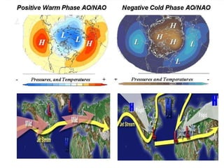
The positive NAO relates to more zonal flow with warmer Atlantic air into Europe and Pacific air into North America. The negative NAO leads to a more meridional pattern with cold air in Siberia often making its way west to western Europe and Cold arctic air over North America trapped over the eastern and central parts of the continent. IceCap 4Sep09
The North Atlantic oscillation (NAO) is a climatic phenomenon in the North Atlantic Ocean of fluctuations in the difference of atmospheric pressure at sea-level between the Icelandic Low and the Azores high . Through east-west oscillation motions of the Icelandic Low and the Azores high , it controls the strength and direction of westerly winds and storm tracks across the North Atlantic. It is highly correlated with the Arctic oscillation , as it is a part of it. The North Atlantic Oscillation is closely related to the Arctic oscillation but should not be confused with the Atlantic Multidecadal Oscillation . [ http:// www.cgd.ucar.edu/cas/jhurrell/indices.html ]
The global temperature has been rising at a steady trend rate of 0.5°C per century since the end of the little ice age in the 1700s (when the Thames River would freeze over every winter; the last time it froze over was 1804). On top of the trend are oscillations that last about thirty years in each direction: 1882 – 1910 Cooling 1910 – 1944 Warming 1944 – 1975 Cooling 1975 – 2001 Warming In 2009 we are where the green arrow points, with temperature leveling off. The pattern suggests that the world has entered a period of slight cooling until about 2030.
This figure from the IPCC TR4 is their summation of the net effects of radiative forcings. Per the IPCC, “Best estimates and uncertainty ranges can not be obtained by direct addition of individual terms due to the asymmetric uncertainty ranges for some factors.” Note that the uncertainty for cloud albedo is almost as large as the total contribution for CO 2 . Using the Stefan-Boltzman constant, 1 Wm -2 ~0.22 O C. Thus the net 1.6 Wm -2 above indicates a 0.35 O C effect. This chart does not include the cooling effect of volcanic aerosols, nor the cooling effect of falling tropospheric relative and specific humidity. The GCR effect could be considered to be represented above in the uncertainty of cloud albedo.
In this image of Atlanta Georgia, blue shows cool temperatures and red shows warm temperatures. Pockets of especially hot temperatures appear in white. (Image courtesy NASA/Goddard Space Flight Center Scientific Visualization Studio.) Image obtained from NASA Earth Observatory webpage -- Ryanjo 00:48, 2 August 2006 (UTC)
The paper Urbanization effects in large-scale temperature records, with an emphasis on China (Jones et al 2008) finds urban temperature trends to be little different to rural trends. The paper begins by looking at 5 sites in and around London. Figure 1 shows absolute temperatures, clearly indicating a UHI influence on the urban sites at London Weather Centre (brown) and St. James Park (dark blue). The coolest record is the rural based Rothamsted (dark green). However, the excess urban warmth has no effect on the temperature trend - all sites show the same overall trend. Dr. Pieke disagrees
Surface temperature trends for 1940 to 1996 from 107 measuring stations in 49 California counties (51,52). The trends were combined for counties of similar population and plotted with the standard errors of their means. The six measuring stations in Los Angeles County were used to calculate the standard error of that county, which is plotted at a population of 8.9 million. The urban heat island effect on surface measurements is evident. The straight line is a least-squares fit to the closed circles. The points marked X are the six unadjusted station records selected by NASAGISS (53-55) for use in their estimate of global surface temperatures. Such selections make NASA GISS temperatures too high. Robinson, et al, “Environmental Effects of Increased Atmospheric Carbon Dioxide”, Journal of American Physicians and Surgeons, (2007)
Land use change impacts the regional and global climate through the surface-energy budget, as well as through the carbon cycle. “The albedo change may be comparable with due to anthropogenic aerosols, solar variation and several of the green house gases.” “Changes in surface vegetation cover can also modify the surface heat fluxes directly.” These aspects are not currently accounted for [by the IPCC].” Roger Pielke et al, 2002
“ The climate-related ecosystem services that tropical forests provide include the maintenance of elevated soil moisture and surface air humidity, reduced sunlight penetration, weaker near-surface winds and the inhibition of anaerobic soil conditions. Roger Pielke et al, 2002
The alteration of tropical landscapes, primarily the conversion of forests to agriculture or pasture, changes the partitioning of solar insolation into its sensible and latent turbulent heat forms. Less transpiration associated with the agricultural and pasture regions results in less thunderstorm activity over this landscape. Roger Pielke et al, 2002
Mount Kilimanjaro’s glaciers have receded dramatically, making the highest point in Africa a high-profile poster child for global warming. Some scientists contend, however, that Kilimanjaro is a poor example, as its glaciers were disappearing before warming set in. American Scientist , July-August 2007 Ice mass had already decreased by 66 percent from 1880 to 1953 — long before global temperatures began to rise rapidly beginning in the 1970s, Solar radiation and sublimation are the primary actors on the mountain’s ice loss. “Deforestation of the mountain's foothills is the most likely culprit because without forests there is too much evaporation of humidity into outer space. The result is that moisture-laden winds blowing across those forests have become drier and drier,“ he explained. “ Loss of humidity automatically leads to a reduction in cloud cover. Clouds play a crucial role in protecting ice from sunrays, with fewer sunrays meaning faster freezing of water.“ Reduced precipitation as another reason for the receding ice cover on the mountain's summit.
This figure from the IPCC TR4 is their summation of the net effects of radiative forcings. Per the IPCC, “Best estimates and uncertainty ranges can not be obtained by direct addition of individual terms due to the asymmetric uncertainty ranges for some factors.” Note that the uncertainty for cloud albedo is almost as large as the total contribution for CO 2 . Using the Stefan-Boltzman constant, 1 Wm -2 ~0.22 O C. Thus the net 1.6 Wm -2 above indicates a 0.35 O C effect. This chart does not include the cooling effect of volcanic aerosols, nor the cooling effect of falling tropospheric relative and specific humidity. The GCR effect could be considered to be represented above in the uncertainty of cloud albedo.
OK. With this backgrowd, let’s specifically address CAGW
What constitutes evidence that carbon-based green house gases, whatever their source, contribute to any significant degree to global warming? There are two tests that will be needed to support this effect.
These are not evidence of global warming induced by well-mixed green house gases.
First, we can look at pre-history in the proxy records.
Here are three hockey stick curves for three well-mixed greenhouse gases, as published by the IPCC. There is a lot of controversy in them, depicting monotonic pre-industrial levels. For example, data clearly show that the rate of rise in methane has stopped about ten years ago, although no one can explain this. But discussing these issues would be a presentation in itself. So, for the sake of argument, we’ll just accept the IPCC position on these GHG levels.
Atmospheric methane concentrations, 1985-2008, with the IPCC methane projections overlaid (adapted from: Dlugokencky et al., 2009
And here is the IPCC third assessment report plot of global temperatures, the famous hockey stick that persists in CAGW proponent position papers to this day. This plot looks an awfully lot like the previous CO2 curve. But remember that correlation is not causation.
The graph first appeared in a paper by Mann, Bradley, and Hughes in 1998 (MBH98) and has appeared as is, or morphed, in many subsequent papers. In MBH98, Mann claimed 1998 to be the warmest year of the millennium, the 1990s to be the warmest decade, and the 20 th century to be the warmest in the last 1,000 years.
Some, including a retired statistician-CEO of a Canadian minerals exploration company, thought it a bit strange. He had been taught that it was cold in Shakespeare's time, but this graph has no indication of the little ice age. He had been taught that the Vikings has settled southern Greenland about one thousand years ago, but this medieval warm period is not shown on Mann’s graph. So he e-mailed Mann and asked for the data. Tree ring data proved to be the key to this mystery.
Stephen McIntyre, Bachelor of Science degree in mathematics from the University of Toronto . He was the president and founder of Northwest Exploration Company Limited and a director of its parent company, Inc. He got curious about the absence of the MWP and LIA and asked to look at the underlying data “rather as I might look at drill data from a mining promotion.” and found that [there was but superficial peer review. Michael E. Mann, PhD, Geophysics, Yale. Pennsylvania State University, Department of Meteorology
Since Mann used government funds, under the freedom of information act, he was compelled to provide the basis for his papers. The ethics of science should have been sufficient.
Mann 98 claimed robustness to [tree rings]. Trees growing at high latitudes or high altitudes are most sensitive to changing temperatures, while the growth of trees in semi-arid environments responds strongly to changing soil water conditions and so provides information on precipitation. Briffa, 2008 “ The hypothesis of a linear relationship between ring widths and world temperature doesn’t hold up.” McIntyre, 2008
Don Graybill published tree ring –temperature data in the early 1980s, but his specimen and original notes were poorly archived and most are lost. So McIntire contacted friends in Colorado (Holzmann) and together they located many of the very trees that Graybill sampled, some like this with Graybills original tags. New core samples were taken.
“ The NAS (National Academy of Sciences) panel warned about strip bark but the shape of these trees has to be seen to be believed. These are not circular trees, but are contorted and asymmetric. The bark may only be a few inches wide. If you’re looking at one of these trees from the side, it’s impossible to guess where the pith is located. One core, which is all that Graybill typically archived, has little chance of establishing the geometry of the tree.” “One of our findings, which to our knowledge is unreported in the scientific literature, is the fantastic difference in ring width chronologies from cores as little as 6 inches from one another, S. McIntyre, Presentation at Ohio State University, May 16, 2008
When the Graybill sites are removed, guess what happened to the hockey stick. It disappeared.
With Mann’s background files now open to public assessment, other interesting data was found. A censored file, showing all other proxies except bristle cone pine tree rings, fail to show any hockey stick trends.
In rebuttal, Mann and the IPCC claimed many other independent studies that show the same hockey stick from tree ring proxies.
The IPCC 4TAR shows this graph, which still includes the discredited MBH09 curve. This “spaghetti plot” is of palaeoclimate temperatures and instrument temperatures of the northern hemisphere, using many proxies including “strip bark” tree rings. McIntyre was able to find the background data for these circled studies.
But the studies were not independent. “One of the obvious defects of these supposedly independent studies is that the same proxies are re-cycled over and over. Here is a re-plot of a figure from Wegman showing that Polar Urals and Tornetrask proxies were used in every reconstruction, while bristlecones or foxtails were used in all but a few.” How do we “know” that 1998 was the warmest year of the millennium? Stephen McIntyre Presentation at Ohio State University May 16, 2008
“ We travelled by helicopter to the upper reaches of the river to be sampled. Small boats were then used for locating and collecting cross-sections from wood exposed along the riverbanks. It was also possible, when going with the stream, to explore the nearest lakes. The best-preserved material from an individual tree is usually found at the base of the trunk, near to the roots. However, many of these remains are radially cracked and it is necessary to tie cross-sections, cut from these trunks or roots, using aluminum wire before sawing. This wire is left in place afterwards as the sections are air-dried.” A continuous multimillennial ring-width chronology in Yamal, northwestern Siberia (PDF) by Rashit M. Hantemirov and Stepan G. Shiyatov
A comparison of Yamal RCS chronologies. red – as archived with 12 picked cores; black – including Schweingruber’s Khadyta River, Yamal (russ035w) archive and excluding 12 picked cores. Steve McIntyre 28Sep09 The graph above shows what happens to the “Hockey Stick” after additional tree ring data, recently released (after a long and protracted fight over data access) is added to the analysis of Hadley’s archived tree ring data in Yamal, Russia.
A comparison of the Briffa chronology of the spaghetti graphs (red) versus the “SChweingruber” variation i.e. using russ035w instead of 12 recent of 252 CRU cores, leaving 240 unchanged. “ The resulting Yamal chronology with its enormous HS blade was like crack cocaine for paleoclimatologists and got used in virtually every subsequent study, including, most recently, Kaufman et al 2009.” Steve McIntyre 28Sep09
“ , instead of the standard negative exponential declining growth, these particular trees started off very slowly, like old trees, and then got a burst of virility when they got to be 100 years old.
Climate modelers have simply assumed that the Earth’s climate system was in a state of energy balance before humans started using fossil fuels. But as is evidenced by the temperature reconstruction for the last 2,000 years (from Loehle, 2007), continuous changes in temperature necessarily imply continuous changes in the Earth’s energy balance. And while changes in solar activity are one possible explanation for these events, it is also possible that there are long-term, internally-generated fluctuations in global energy balance brought about by natural cloud or water vapor fluctuations. For instance, a change in cloud cover will change the amount of sunlight being absorbed by the Earth, thus changing global temperatures. Or, a change in precipitation processes might alter how much of our main greenhouse gas — water vapor — resides in the atmosphere. Changes in either of these will cause global warming or global cooling. July 13th, 2009 Roy Spencer, “How do Climate Models Work”
modern view of a pass in the Alps (with glacier lines of 1922 and 1856) Steven McIntyre at Ohio State, 2008 reconstructed view in Roman times of 2000 years ago Schlüchter and Jörin (2004). The longest retreat phase of glaciers of the Swiss glaciers was about 2000 years ago correlating with studies by Holzhauser et al. (2005) and Joerin et al. (2006). The glaciers reached their maximum extent of the second half of the Holocene during the LIA.
In modern times, we don’t need to rely on proxy indicator of temperature; we can measure it directly. This is done with ground-base thermometers, with devices that measure the temperature of ocean waters, with balloons that transmit temperature as they ascend into the atmosphere, and with satellites that use microwaves to probe the lower troposphere.
Radiosonde-based layer temperatures (T850-300, T100-50) are height-weighted averages of the temperature in those layers. Satellite-based temperatures (T2LT, T2, and T4) are mass-weighted averages with varying influence in the vertical as depicted by the curved profiles, i.e., the larger the value at a specific level, the more that level contributes to the overall satellite temperature average. Layer temperatures vary from equator to pole so the pressure and altitude relationship here is based on the atmospheric structure over the conterminous U.S.
From Wikipedia, This image shows the instrumental record of global average w:temperatures as compiled by the w:NASA 's w:Goddard Institute for Space Studies . The data set used follows the methodology outlined by Hansen, J., et al. (2006) &quot;Global temperature change&quot;. Proc. Natl. Acad. Sci. 103: 14288-14293. Following the common practice of the w:IPCC , the zero on this figure is the mean temperature from 1961-1990. This presentation is one of the foundations to support Hansen’s contention that the 1990 were the warmest in a millennium, or at least during the industrial age.
And so, despite a constant rise in atmospheric CO 2 , the temperature rise during the period of alarm noted by James Hansen of GISS has not been dramatic. The impact of natural events, like the injection of cooling volcanic aerosols into the atmosphere and the major 1997 – 1998 El Nino, are visible. But this decade has not warmed despite more CO 2 in the atmosphere and despite the lack of cooling volcanic aerosols.
But there is other data, like this, where many recall the hot 1930s. When examined on a state by state basis, the 1930s jumps out as the warmest decade with 24 state records. 37 records occurred before the 1970s IceCap 2Aug09
The disparity lies in how temperatures are measured.
Here is the NCDC example of a [desired] typical instrument site configuration. The wind shield around the precipitation gauge helps to improve the accuracy of the liquid and frozen precipitation catches.
And here is an example of a well-executed weather station site.
More typical is this National Weather Service weather station site.
Anthony Watts, a meteorologist in California, wondered about the precision of the data used to construct the GISS historic temperature curve. So he organized a group across the nation to check out each weather station site used by GISS to build their curve of temperature history. And the next few slides represent what he found. They are self-explanitory.
Buffalo Bill Dam, Cody WY shelter on top of a stone wall at the edge of the river. It is surrounded by stone building heat sinks except on the river side. On the river it is exposed to waters of varying temperatures, cold in spring and winter, warm in summer and fall as the river flows vary with the season. The level of spray also varies, depending on river flow. http://wattsupwiththat.wordpress.com/2008/07/15/how-not-to-measure
taken at Roseburg, OR (MMTS shelter on roof, near a/c exhaust) http://www.surfacestations.org/images/Roseburg_OR_USHCN.jpgPhoto
Surfacestations project reaches 82% of the network surveyed. 1003 of 1221 stations have been examined in the USHCN network. U.S. Department of Commerce National Oceanic and Atmospheric Administration (NOAA) National Environmental Satellite, Data, and Information Service (NESDIS) CRN = Climate Reference Network
“ Station drop-out has occurred– from a peak of 6,000 stations in 1970 to 2,000 today. The biggest drop-off occurred around 1990. The plot was made with downloaded GHCN 2 data with annual mean global temperature in degrees Celsius and number of stations. Many of the stations that were dropped were rural. A larger percentage of the stations remaining were urban.” Joseph D’Aleo, Fellow of the AMS, CCM, WSI, Icecap WUWT 11Aug09
Every dot on a plot represents a station, not a scribal record. Stations may be comprised of multiple records. A blue dot represents a station with an annual average that was fully calculated from existing monthly averages. A red dot represents a station that had missing monthly averages for that year, so the annual average had to be estimated. Stations that had insufficient data to estimate an annual average are not shown. Historical Station Distribution by John Goetz on February 10th, 2008
1905 shows improved coverage across the continental US, Japan and parts of Australia. A few stations have appeared in Africa. Historical Station Distribution by John Goetz on February 10th, 2008
1925 shows increased density in the western US, southern Canada, and the coast of Australia. Historical Station Distribution by John Goetz on February 10th, 2008
At the end of WWII, not a lot of change is noticeable other than improved coverage in Africa and South America as well as central China and Siberia. Historical Station Distribution by John Goetz on February 10th, 2008
In 1965 we see considerable increases inChina, parts of Europe, Turkey, Africa and South America. Historical Station Distribution by John Goetz on February 10th, 2008
A decline in quality seems to be apparent in 1985, as many more stations show as red, indicating their averages are estimated due to missing monthly data. Historical Station Distribution by John Goetz on February 10th, 2008
A huge drop in stations is visible in the 2005 plot, notably Australia, China, and Canada. 2005 was the “ warmest year ” in over a century. Not surprising, as the Earth hadn't seen station coverage like that in over a century. Historical Station Distribution by John Goetz on February 10th, 2008
The final plot illustrates the world-wide station coverage used to tell us &quot; 2006 Was Earth's Fifth Warmest Year &quot;. Historical Station Distribution by John Goetz on February 10th, 2008
An Alternative Explanation for Differential Temperature Trends at the Surface and in the Lower Troposphere, Philip J. Klotzbach et al, August, 2009, Journal of Geophysical Research Trends in thermometer-estimated surface warming have been larger than trends in the lower troposphere estimated from satellites and radiosondes . The land surface temperature record does in fact combine temperature minimum and maximum temperature measurements. Where there has been a reduction in nighttime cooling, the long-term temperature record will have a warm bias. The warm bias will represent an increase in measured temperature due to a local redistribution of heat through a causal mechanism distinct from the large-scale radiative effects of greenhouse gases. However it will not represent an increase in the accumulation of heat in the deep atmosphere..
Argo is an international collaboration that collects high-quality temperature and salinity profiles from the upper 2000m of the ice-free global ocean and currents from intermediate depths. The data come from battery-powered autonomous floats that spend most of their life drifting at depth where they are stabilized by being neutrally buoyant at the &quot;parking depth&quot; pressure by having a density equal to the ambient pressure and a compressibility that is less than that of sea water.
At typically 10-day intervals, the floats pump fluid into an external bladder and rise to the surface over about 6 hours while measuring temperature and salinity. Satellites determine the position of the floats when they surface, and receive the data transmitted by the floats. The bladder then deflates and the float returns to its original density and sinks to drift until the cycle is repeated. Floats are designed to make about 150 such cycles.
Ocean temperatures have only been measured properly from mid 2003, when the Argo network became operational. Over 3,000 Argo floats cover all the world’s oceans. They dive down to measure temperatures, then resurface to radio back the information. The previous XBT system did not monitor huge areas of ocean, did not go as deep, and was much less accurate. Dr. David Evans, ICECAP, 31Jul09
From Real Climate, Gavin Schmidt 19Jun09 “ Global SLR [sea level rise] is a product of (in rough order of importance) ocean warming, land ice melting, groundwater extraction/dam building, and remnant glacial isostatic adjustment (the ocean basins are still slowly adjusting to the end of the last ice age). “ Ocean heat content trends largely reflect the planetary radiative imbalance.
“ There is an annual periodicity in the data, probably due to the north-south asymmetry in ocean area and the effect of orbital variations over the year. The peak-to-trough amplitude of the model is 6.30 x 10 22 Joules (J) at the beginning of the period and declines to 3.88 x 10 22 J at the end, showing a damping of the cycle over the 4.5-year period. The slope of the linear component of the model is -0.35 x 10 22 J/yr. This result clearly excludes warming as a possible interpretation of this data . It has previously been estimated by Willis et al. (2004) that from 1993 to 2003 the upper ocean gained 8.1 (±1.4) x 10 22 J of heat. This study estimates a loss since then of from 0.668 to 2.48 x 10 22 J, or 19.4% (up to 31%) of the gain of the prior decade.
These figures reveal a robust failure on the part of the [NASA] GISS model to project warming. The heat deficit shows that from 2003-2008 there was no positive radiative imbalance caused by anthropogenic forcing, despite increasing levels of CO 2 . Indeed, the radiative imbalance was negative, meaning the earth was losing slightly more energy than it absorbed. Solving for Riin Eq. #1, the average annual upper ocean radiative imbalance ranged from a statistically insignificant -.07 W/m2 (using Willis) to -.22 W/m2(using Loehle). William DiPuccio , WUWT July 2009
Global OHC has dropped back to its 2003 levels. Data from National Oceanic Data Center, via Bob Tisdale 4Oct09
“ Earth’s radiation imbalance by analyzing three recent independent observational ocean heat content determinations for the period 1950 to 2008 and compare the results with direct measurements by satellites. A large annual term is found in both the implied radiation imbalance and the direct measurements. Its magnitude and phase confirm earlier observations that delivery of the energy to the ocean is rapid , thus eliminating the possibility of long time constants associated with the bulk of the heat transferred. Longer-term averages of the observed imbalance are not only many-fold smaller than theoretically derived values, but also oscillate in sign. These facts are not found among the theoretical predictions.” Ocean heat content and Earth’s radiation imbalance D.H. Douglass and R, S, Knox
The ocean heat flux is indeed reflected by sea surface temperatures measured by satellite, which show that the oceans have not warmed since the last major El Nino event in 1998.
Icecap Note: to enable them to make the case the oceans are warming, NOAA chose to remove satellite input into their global ocean estimation and not make any attempt to operationally use Argo data in the process. This resulted in a jump of 0.2C or more and ‘a new ocean warmth record’ in July.
August 2009 SST for the NOAA satellite-based OI.v2 SST dataset were not records. NOAA writes about the Optimum Interpolation (OI.v2) data, “The optimum interpolation (OI) sea surface temperature (SST) analysis is produced weekly on a one-degree grid. The analysis uses in situ and satellite SST’s plus SST’s simulated by sea-ice cover. http://www.cdc.noaa.gov/data/gridded/data.noaa.oisst.v2.html Note that this data indicates the seas are have not warmed in the last decade.
The Hadley Centre’s HADSST2 does not show record SST anomalies for July, August, or for the Summer of 2009. Far from it. Refer to Figure 5. The Hadley Centre uses different techniques to smooth and infill missing data. The differences between the Hadley Centre and NOAA methodologies are explained in the NOAA paper about the ERSST.v3b data, “ Improvements to NOAA’s Historical Merged Land-Ocean Surface Temperature Analysis (1880-2006) ”. It appears that the methods used by NOAA to calculate Global SST in their ERSST.v3b dataset and the removal of the satellite data from those calculations created an upward bias.
“ As can be seen, at least for the time being, temperatures have returned to the long-term average. Of course, this says nothing about what will happen in the future. I have also plotted the linear trend line, which is for entertainment purposes only. The SSTs come from the AMSR-E instrument on NASA’s Aqua satellite, and are computed and archived at Remote Sensing Systems (Frank Wentz). I believe them to be the most precise record of subtle SST changes available, albeit only since mid-2002.” Roy Spencer, UAH, 16Oct09 in WUWT
The following chart from a presentation by Dr. Richard Lindzen shows prediction results from a number of climate models and satellite data. The horizontal axis shows the change in sea surface temperatures per year as measured over various time intervals. The vertical axis is the change in outgoing longwave radiation at the top of the atmosphere as predicted by several climate models. A positive correlation (slope from bottom left to top right) indicates that there is a negative feedback loop in SST change such that the hotter the sea gets the more heat is radiated away to space, which reduces the temperature rise. A negative correlation (slope from top left to bottom right) indicates that there is a positive feedback loop in that the atmosphere inhibits heat loss to space, which increases the temperature further. 11 GCM are not in agreement with the empirical data.
Here is NASA’s GISS view of historic CO 2 . It is subject to serious challenge, but for this discussion is indicative of the recent rise of CO 2 globally. Yet the temperature signature has not followed this rise.
But CO 2 is a green house gas, and there is no debate that, without other forcings, it will heat the atmosphere. The question is how much.
James Hansen says anthropogenic forcings, mainly GHG which is mainly CO2, heat the atmosphere ~2 Wm -2 .
Theoretically, in a dry atmosphere, carbon dioxide could absorb about three times more energy than it actually does. Clouds, in the absence of all other greenhouse gases, could do likewise. Note that the temperature effect of atmospheric carbon dioxide is logarithmic . If we consider the warming effect of the pre-Industrial Revolution atmospheric carbon dioxide (about 280 ppmv) as 1, then the first half of that heating was delivered by about 20ppmv (0.002% of atmosphere) while the second half required an additional 260ppmv (0.026%). To double the pre-Industrial Revolution warming from CO2 alone would require about 90,000ppmv (9%) but we'd never see it - CO2 becomes toxic at around 6,000ppmv (0.6%, although humans have absolutely no prospect of achieving such concentrations).
Here are three views of the logarithmic effect of atmospheric CO 2 , each presuming that there are no other forcings. Charnock and Shine, who are widely referenced, Require humanity to completely take over all natural effects that were operating before the Industrial Revolution; this of course, is illogical. On the other end is Lindzen, who projects but a 0.5 O C increase from a doubling of CO 2 from current levels, given a clear sky condition. But of course this is not reality as other things like clouds are indeed factors. With 40% clouds, Lindzen estimates a doubling of CO 2 would add only 0.22 O C to the earth’s temperature.
The effect of carbon dioxide on temperature is logarithmic and thus climate sensitivity decreases with increasing concentration. The first 20 ppm of carbon dioxide has a greater temperature effect than the next 400 ppm. The rate of annual increase in atmospheric carbon dioxide over the last 30 years has averaged 1.7 ppm. From the current level of 380 ppm, it is projected to rise to 420 ppm by 2030. The projected 40 ppm increase reduces emission from the stratosphere to space from 279.6 watts/m2 to 279.2 watts/m2. Using the temperature response demonstrated by Idso (1998) of 0.1°C per watt/m2, this difference of 0.4 watts/m2 equates to an increase in atmospheric temperature of 0.04°C. David Archibald, March 2009
Since the beginning of the Industrial Revolution, increased atmospheric carbon dioxide has increased the temperature of the atmosphere by 0.1°. This isn’t much, in fact it is almost next to nothing. To the end of time, and let’s call that 1,000 ppm of carbon dioxide in the atmosphere, the total effect might be good for 0.4 degrees. It is hard to get excited or concerned about such a number. It is swamped by natural variability, for example the two degree temperature range of the 20th century, and the two degree temperature fall to come over the next decade. David Archibald, March, 2009
annotated to show the 350 PPM desired by activists, versus the 388 PPM (MLO seasonally corrected value) where we are now:
Here is the same graph, annotated again with intersecting lines and values, and zoomed on the areas of interest. Depending on whether you believe the models or the actual observations determines what value would be gained from a reduction to 350 PPM. For belief in the models we’d get approximately 0.5°C drop in temperature. For belief in the observations (RSS HadCRUT3 data) we’d get approximately 0.3°C drop in temperature. As a side note, the 350PPM target was Dr. Jim Hansen’s idea:
Absorption of ultraviolet, visible, and infrared radiation by various gases in the atmosphere. Most of the ultraviolet light (below 0.3 microns) is absorbed by ozone (O3) and oxygen (O2). Carbon dioxide has three large absorption bands in the infrared region at about 2.7, 4.3, and 15 microns. Water has several absorption bands in the infrared, and even has some absorption well into the microwave region. There is already sufficient CO2 in the atmosphere to absorb almost all of the radiation from the sun or from the surface of the earth in the principal CO2 absorption bands. (Data from ref. [1], page 93; original data are from Howard et al [21] and Goody [22]).
The bulk of Earth's greenhouse effect is due to water vapor by virtue of its abundance. Water accounts for about 90% of the Earth's greenhouse effect -- perhaps 70% is due to water vapor and about 20% due to clouds (mostly water droplets), some estimates put water as high as 95% of Earth's total tropospheric greenhouse effect (e.g., Freidenreich and Ramaswamy, “Solar Radiation Absorption by Carbon Dioxide, Overlap with Water, and a Parameterization for General Circulation Models,” Journal of Geophysical Research 98 (1993):7255-7264).
Another source sums the differing views on the impact of CO 2 as shown on this table.
“ While it is intuitively reasonable that the most prolific and important greenhouse gas could act as a magnifier there is no evidence that it does. In fact water vapor is self limiting because it precipitates out as rain and snow and its effect also varies as cloud, with more bright low cloud acting as a cooling effect. only the synchronous warming and subsequent cooling depicted in the atmospheric series and near-surface land and sea surface datasets of ~0.9 and ~0.5 K respectively. Since the world cooled almost as abruptly as it warmed we can only assume no positive feedback mechanism was invoked and thus Earth is not perilously perched upon some critical temperature threshold beyond which new physics takes over and runaway enhanced greenhouse warming becomes a self-perpetuating nightmare. That test for a multiplier effect surely failed.” Junk Science, August, 2007
Per the IPCC and all of their models, a doubling of CO 2 and their hypothesized water amplification must cause an atmospheric warming especially in the lower troposphere over the tropics; this would be around 400 mb to 300 mb or about 9 km altitude.
But this warming has not happened. The mystery of the missing hot spot is solved by the Miskolczi greenhouse effect theory [hypothesis] and confirmed by the declining relative humidity, especially at the altitude of the predicted hot spot. The declining relative humidity reduces the temperature compared to the model projections so there is no hot spot. The GCM assumption of constant relative humidity is wrong and is yet another proof that the climate predictions of the IPCC are wrong. Ken Gregory, July 2009, “The Saturated Greenhouse Effect”
This graph shows that the relative humidity has been dropping, especially at higher elevations allowing more heat to escape to space. The curve labelled 300 mb is at about 9 km altitude, which is in the middle of the predicted (but missing) tropical troposphere hot-spot. This is the critical elevation as this is where radiation can start to escape without being recaptured. The average annual relative humidity at this altitude has declined by 21.5% from 1948 to 2007!
“ The actual water vapour content (specific humidity) in the upper troposphere has declined by 17% from 1948 to 2008 at the 400 mb pressure level. The climate models predict that humidity will increase in the upper troposphere, but the data shows a large decrease, just where water vapour changes have the greatest effect on global temperatures. ” through Ken Gregory 3Sept09
And so the representation of the predictions made by James Hansen to the US Congress in 1988, has not materialized; here we see Hansen’s projection plotted against how the climate actually behaved. Pretty much what one would expect if the sensitivity of the model was set too high, Warming Caused by Soot, Not CO2 From the Resilient Earth Submitted by Doug L. Hoffman on Wed, 07/15/2009 – 13:19
http://climatesci.org/ May, 2009 Review of the Congressional Budget Office “The Expected Impacts of Climate Change in the United States” by Roger A. Pielke Sr. January 14 2009 The observational data in the last decade conflict with the finding reported in the CBO draft report. For example, the global average lower tropospheric temperatures have not increased for at least 7 years, and indeed, show a recent decline. See (from http://www.ssmi.com/msu/msu_data_description.html ). There is no acceleration of warming. Studies of the surface temperature data are similarly finding a lack of accelerated warming, and, in fact, are even finding that for the last 8 years or so, that the IPCC model predictions of the global average surface temperature trend are not consistent with the observations. Moreover, there is new evidence of a significant warm bias in the land portion of the surface temperature data base that is used to construct the global average trend (e.g., see Pielke et al. 2007; Lin et al. 2007)
Here is a plot of the counter trending rising CO2 with decreasing atmospheric temperature; this from satellites.
The falling temperature is also noted in data from ground stations, this from Great Britain's Hadley Center. * Air temperatures have been falling for years. Satellites show that 1998 was the warmest recent year and that a cooling trend started in 2002 . Dr. David Evans , ICECAP, 31July09 Summary for Policymakers
Robinson, et al, “Environmental Effects of Increased Atmospheric Carbon Dioxide”, Journal of American Physicians and Surgeons, (2007) Present GHE is the current green house effect from all atmospheric phenomena. “Radiative effect of CO2” is the added greenhouse radiative effect from doubling CO2 without consideration of other atmospheric components. “Hypothesis 1 IPCC” is the hypothetical amplification effect assumed by IPCC, “Hypothesis 2” is the hypothetical moderation effect.
The Vostok record shows that changes in CO2 happen after corresponding changes in T. This lag is shown most clearly by large-amplitude features in the more recent portion of the record: CO2 rises hundreds of years after T rises, and falls thousands of years after T falls. CO2 at a given time cannot affect the level of T that existed hundreds-to-thousands of years earlier. CO2 is in temperature-dependent time-lagged equilibrium, and that the temperature dependence of CO2 is essentially linear through the Vostok range. Atmospheric Temperature and Carbon Dioxide: Feedback or Equilibrium? R. Taylor as reported on 24Aug09 in WUWT
Looking at the detail of ice core data teases out the lag of CO2 following changes in atmospheric temperature. This is from the IPCC’s 4TAR.
T and CO2 appear to have been in equilibrium until about 3,000 BCE. Over the 5,000 years since then, CO2 has risen increasingly above its natural equilibrium. By 1,800 CE, CO2 had risen to a level comparable to the highest in the Vostok record. During this time, T declined at a rate of 0.1 °C per thousand years, indicating again that CO2 has no apparent effect on T. The trends of this 5,000-year interval of excess CO2 are consistent with the equilibrium model, in which T is independent of CO2.
Despite the high degree of mixing that occurs with carbon dioxide, the regional patterns of atmospheric sources and sinks are still apparent in mid-troposphere carbon dioxide concentrations.
Consider CO2, a GHG uniformly dispersed around the globe [CO2 shows a variation with latitude which is less than 4% from pole to pole [1] ]. If CO2 is the driver of global warming, then its impact should be globally uniform. Douglas el al [2] show with satellite microwave sounding data that it is not uniform, with the northern hemisphere showing between 1979-2007 a temperature increase trend four times (0.28 O K/decade) that of the tropics and southern hemisphere (~0.07 O K/decade). [1] Earth System Research Laboratory. 2008 Global distribution of atmospheric carbon dioxide. NOAA http:// www.esrl.noaa/gov [2] Limits on CO2 Climate Forcing from Recent Temperature Data of Earth, Energy and Environment, Aug 2008.
This figure from the IPCC TR4 is their summation of the net effects of radiative forcings. Per the IPCC, “Best estimates and uncertainty ranges can not be obtained by direct addition of individual terms due to the asymmetric uncertainty ranges for some factors.” Note that the uncertainty for cloud albedo is almost as large as the total contribution for CO 2 . Using the Stefan-Boltzman constant, 1 Wm -2 ~0.22 O C. Thus the net 1.6 Wm -2 above indicates a 0.35 O C effect. This chart does not include the cooling effect of volcanic aerosols, nor the cooling effect of falling tropospheric relative and specific humidity. The GCR effect could be considered to be represented above in the uncertainty of cloud albedo.
“ Carbon dioxide is not even a little bit bad. It is wholly beneficial. This graph from a recent Idso paper shows plant growth response to atmospheric carbon dioxide enrichment. The 100 ppm carbon dioxide increase since the beginning of industrialisation has been responsible for an average increase in plant growth rate of 15% odd. The 50% increase in plant growth rate due to a 300 ppm increase in atmospheric carbon dioxide can be expected about the middle of the next century. What a wonderful time that will be.”. David Archibald, March, 2009
CO2 is a major plant fertilizer. The increase in CO2 emissions have caused increased crop yields and faster growing plants and forests, thereby greening the planet. Estimates vary, but somewhere around 15% seems to be the common number cited for the increase in global food crop yields due to aerial fertilization with increased carbon dioxide since 1950. Commercial growers deliberately generate CO2 and increase its levels in agricultural greenhouses to between 700 ppm and 1,000 ppm to increase productivity and improve the water efficiency of food crops far beyond those in the somewhat CO2 starved atmosphere. Ken Gregory citing Idso’s reviews.
In a world of higher atmospheric carbon dioxide, crops will use less water per unit of carbon dioxide uptake, and thus the productivity of semi-arid lands will increase the most. Craig Idso
What constitutes evidence that carbon-based green house gases, whatever their source, contribute to any significant degree to global warming? There are two tests that will be needed to support this effect.