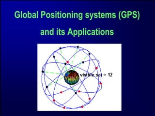
3. Global Positioning S t
Gl b l P iti i System (GPS)
In 1973 the U.S. Department of Defense
decided to establish, develop, test, acquire,
and deploy a spaceborne Global Positioning
System (GPS). The result of this decision is the
p
present NAVSTARGPS (NAVigation Satellite
( g
Timing And Ranging Global Positioning
System).
4. GPS General Characteristics
Developed by the US
Department of Defense
D t t fD f
Provides
Accurate Navigation
g
10 - 20 m
Worldwide Coverage
24 hour access
Common Coordinate
System
Designed t replace existing
D i d to l i ti
navigation systems
Accessible by Civil and Military
5. GPS Tidbits
Development costs estimate ~$12 billion
Annual operating cost ~$400 million
$400
3 Segments:
Space: Satellites
User: Receivers
Control: Monitor & Control stations
Prime Space Segment contractor: Rockwell International
Coordinate Reference: WGS-84
Operated by US Air Force Space Command (AFSC)
Mission control center operations at Schriever (formerly
Falcon) AFB, Colorado Springs
6. GPS System
Components
C t
Space Segment
NAVSTAR : NAVigation
Satellite Time and Ranging
24 Satellites (30)
20200 Km
Control Segment
User Segment
g 1 Master Station
Receive Satellite Signal 5 Monitoring Stations
7. Control Segment
g
Monitor and Control
Colorado
Springs
Ascension Kwajalein
Hawaii
Islands
Diego
Master Control Station Garcia
Monitor Station
Ground Antenna
8. GPS Segments
Space Segment
Satellite Constellation
User Segment
Ground
Antennas
Monitor
AFSCN
Stations
Master Control Station
FAIRBANKS
ENGLAND
Control Segment COLORADO SPRINGS
SOUTH
USNO WASH D.C.
KOREA
VANDENBERG, AFB
CAPE CANAVERAL
BAHRAIN
Master Control Station (MCS) Advanced Ground Antenna HAWAII Master C
Control S i
l Station
KWAJALEIN
ASCENSION
Ground Antenna (GA) Monitor Station (MS) ECUADOR DIEGO
GARCIA
TAHITI
National Geospatial-Intelligence Agency (NGA) Tracking Station
Geospatial- SOUTH
ARGENTINA AFRICA
Alternate Master Control Station (AMCS) NEW ZEALAND
9. Space Segment
p g
24 Satellites • 12 Hourly orbits
4 satellites in 6 Orbital – In view for 4-5 hours
45
Planes inclined at 55 • Designed to last 7.5 years
Degrees • Different Classifications
20200 Km above the Earth
K b th E th – Block 1, 2, 2A, 2R & 2 F
55
Equator
q
10. User Segment
The most visible segment
GPS receivers are found in many
locations and applications
11. How It Works (In 5 Easy Steps)
( y p )
GPS is a ranging system (triangulation)
The “ f
Th “reference stations” are satellites moving at 4 k /
t ti ” t llit i t km/s
1. A GPS receiver (“the user”) detects 1-way ranging signals
from several satellites
Each transmission is time-tagged
Each transmission contains the satellite’s position
2. The time-of-arrival is compared to time-of-transmission
3. The delta-T is multiplied by the speed of light to obtain the
range
4. Each range puts the user on a sphere about the satellite
5. Intersecting several of these y
g yields a user p
position
13. Outline Principle : Position
The satellites are like “Orbiting Control Stations
Orbiting Stations”
Ranges (distances) are measured to each satellite
using time dependent codes
Typically GPS receivers use inexpensive clocks They
clocks.
are much less accurate than the clocks on board the
satellites
A radio wave travels at the speed of light
(
(Distance = Velocity x Time)
y )
Consider an error in the receiver clock
1/10 second error = 30,000 Km error
1/1,000,000 second error = 300 m error
14. Timing
Accuracy of position is only as good as your clock
To know where you are, you must know when you receive.
Receiver clock must match SV clock to compute delta-T
SVs carry atomic oscillators (2 rubidium, 2 cesium each)
Not practical for hand-held receiver
Accumulated drift of receiver clock is called clock bias
The
Th erroneously measured range i called a pseudorange
l d is ll d d
To eliminate the bias, a 4th SV is tracked
4 equations 4 unknowns
equations,
Solution now generates X,Y,Z and b
If Doppler also tracked, Velocity can be computed
15. Position Equations
P1 = ( X − X 1 ) 2 + (Y − Y 1 ) 2 + ( Z − Z 1 ) 2 + b
P2 = (X − X 2 ) 2 + (Y − Y 2 ) 2 + ( Z − Z 2 ) 2 + b
P3 = ( X − X 3 ) 2 + (Y − Y 3 ) 2 + ( Z − Z 3 ) 2 + b
P4 = (X − X 4 ) 2 + (Y − Y 4 ) 2 + ( Z − Z 4 ) 2 + b
Where:
Pi = Measured PseudoRange (Biased ranges) to the ith SV
Xi , Yi , Zi = Position of the ith SV, Cartesian Coordinates
,
X , Y , Z = User position, Cartesian Coordinates, to be solved-for
b = User clock bias (in distance units), to be solved-for
The above nonlinear equations are solved iteratively using an initial
estimate of the user position, XYZ, and b- same for all satellites
16. Point Positioning
Accuracy 10 - 100 m
A receiver in autonomous mode provides navigation and
positioning accuracy of about 10 to 100 m due to the
effects of GPS errors!!?
ff t f !!?
17. The Almanac
In addition to its own nav data, each SV also
broadcasts info about ALL the other SV’s
In a reduced-accuracy format
Known as the Almanac
Permits receiver to predict, from a cold start,
“where to look” for SV’s when powered up
GPS orbits are so predictable, an almanac may be
valid for months
Almanac data is large
12.5 minutes to transfer in entirety
18. GPS Signals
Most unsophisticated receivers track only L1
M hi i d i k l
If L2 tracked, then the phase difference (L1-L2) can
be
b used t filt out i
d to filter t ionospheric d l
h i delay.
This is true even if the receiver cannot decrypt the P-
code (more later)
L1-only receivers use a simplified correction model
19. GPS Error Sources
(uncertainities based on Satellite, signal propagation, and receiver based)
Standard Positioning Service (SPS ):
Satellite clocks: < 1 to 3.6 meters
Orbital errors: < 1 meter
Receiver noise: 0.3 to 1.5 meters
Ionosphere: 5.0 to 7.0 meters
Troposphere: 0.5 to 0.7 meters
Multipath: undetermined
User error: Up to a kilometer or more
Errors are cumulative
20. Satellite Geometry
y
Satellite geometry can affect the quality of signals and
g y q y g
accuracy of receiver trilateration.
Positional Dilution of Precision (PDOP) reflects each
satellite’s position relative to the other satellites being
accessed by a receiver.
PDOP can b used as an i di t
be d indicator of th quality of a
f the lit f
receiver’s triangulated position.
It s
It’s usually up to the GPS receiver to pick satellites which
provide the best position trilateration.
Some receivers do allow PDOP manipulation by the user.
p y
21. Dilution of Precision (DOP)
Satellite geometry can affect the quality of signals and accuracy of
receiver trilateration.
• A description of purely geometrical contribution to the uncertainty in
a position fix.
• It is an indicator as to the geometrical strength of the satellites being
tracked at the time of measurement
– GDOP (Geometrical)
• Includes Lat, Lon, Height & Time Good GDOP
– PDOP (Positional) Poor DOP
• Includes Lat, Lon & Height
– HDOP (Horizontal)
• Includes Lat & Lon
– VDOP (Vertical)
• Includes Height
QUALITY DOP
Very Good
V G d 1-3
13
Good 4-5
Fair 6
Suspect >6
26. Satellite Mask Angle
Atmospheric Refraction is greater for satellites at
angles that are low to the receiver because the
signal must pass through more atmosphere.
There is a trade off between mask angle and
atmospheric refraction. Setting high angles will
t h i f ti S tti hi h l ill
decrease atmospheric refraction, but it will also
decrease the possibility of tracking the
necessary four satellites.
29. Signal Obstruction
When something blocks the GPS signal.
Areas of Great Elevation Differences
Canyons
Mountain Obstruction
Urban Environments
Indoors
30. Selective Availability (SA)
To deny high-accuracy realtime positioning to potential enemies,
DoD reserves the right to deliberately degrade GPS performance
Only on the C/A code
By far the largest GPS error source
Accomplished by:
“Dithering” the clock data
Results in erroneous pseudoranges
Truncating the nav message data
Erroneous SV positions used to compute user position
Degrades SPS solution by a factor of 4 or more
Long-term averaging is the only effective SA compensator
ON 1 MAY 2000: SA WAS DISABLED BY DIRECTIVE
31. Selective Availability (SA)
100m
• In theory a point position can be 30m
accurate to 10 - 30 b
t t 30m based on
d
the C/A Code
The USDoD degrades the
accuracy of the broadcast
f th b d t
information P
Dither the Satellite
Clocks
Satellite Orbital
Information +/-
+/- 100m (95%)
Positional accuracy P = True Position
100m (95%)
33. Error Budget
E B d t
Typical Error in Meters (per satellite)
Standard GPS Differential GPS
Satellite Clocks 1.5 0
Orbit Errors 2.5
25 0
Ionosphere 5 0.4
Troposphere 0.5 0.2
Receiver Noise 0.3 0.3
Multipath 0.6 0.6
SA 30 0
Typical P i i A
T i l Position Accuracy
Horizontal 50 1.3
Vertical 78 2
3-D
3D 93 2.8
28
Trimble Navigation Limited
34. How do I
Improve my Accuracy ?
Use
Differential GPS
(
(Receiver position, satellite position, frequency-
p p frequency-
q y
ionospheric corrections, time-ambiguity of carrier phase
time-
measurements)
35. Differential Positioning
g
It is possible to determine the
position of Rover ‘B’ in relation to
Reference ‘A’ provided
– The coordinates of the
Reference Station (A) are
known
– Satellites are tracked
simultaneously
• Differential Positioning
– eliminates errors in the
sat. and receiver clocks A B
– minimizes atmospheric
delays
– A
Accuracy 0 5 cm - 5 m
0.5
36. Differential Positioning
If using Code only
accuracy is in the
range of 0 5m - 5
0.5m
m
This is typically
yp y
referred to as
DGPS
A B
38. Summary of GPS Positioning
y g
• Point Positioning Methods using stand alone receivers
provide 10 - 100 m accuracy
– Dependent on SA
– 1 Epoch solution
• Differential Positioning Methods using 2 receivers,
simultaneously tracking a minimum of 4 satellites
y g
(preferably 5) will yield 0.5 cm to 5 m accuracy with respect
to a Reference Station
• Differential Techniques using Code will give meter accuracy
• Differential Techniques using Phase will give centimeter
accuracy
39. GPS Surveying Techniques
Static
St ti
For long baselines (>20Km), where the highest
possible accuracy is required
This i th t diti
Thi is the traditional t h i
l technique f providing
for idi
Geodetic Networks
The only solution for large areas
Rapid Static
For baselines up to 20Km
Short Occupation times
Normally used for high production
40. GPS Surveying Techniques
y g q
Stop and Go
Detail Surveys. Any application
Surveys
where many points close
together have to be surveyed
Fast and economical
Ideal for open areas
Kinematic
Used to track the trajectory of a
moving object (continuous
measurements)
Can be used to profile
roadways, stockpiles, etc.
41. References
R f
http://www.glonass-
ianc.rsa.ru/pls/htmldb/f?p=202:1:15000421459964108253
http://igscb.jpl.nasa.gov/
http://igscb jpl nasa gov/
http://www.navcen.uscg.gov/gps/precise/default.htm
Interface Control Documents:
http://www.navcen.uscg.gov
http://www.Glonass-ianc.ras.ru
htt // Gl i
http://www.Galileoju.com