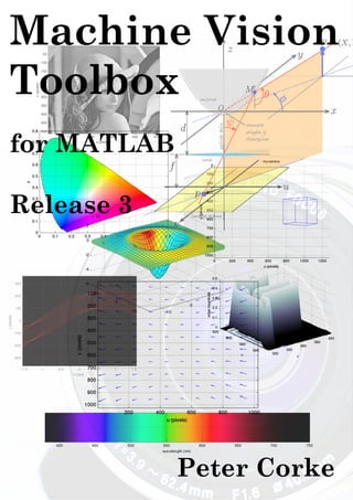
Machine Vision Toolbox for MATLAB (Relese 3)

Release
Release date

3.3
October 2012

Licence
Toolbox home page
Discussion group

LGPL
http://www.petercorke.com/robot
http://groups.google.com.au/group/robotics-tool-box

Copyright c 2012 Peter Corke
peter.i.corke@gmail.com
http://www.petercorke.com

Preface

Peter Corke

Peter C0rke

Robotics,
Vision
and
Control

isbn 978-3-642-20143-1

9 783642 201431

›

springer.com

Corke

1
Robotics, Vision and Control

The practice of robotics and computer vision
each involve the application of computational algorithms to data. The research community has developed a very large body of algorithms but for a
newcomer to the field this can be quite daunting.
For more than 10 years the author has maintained two opensource matlab® Toolboxes, one for robotics and one for vision.
They provide implementations of many important algorithms and
allow users to work with real problems, not just trivial examples.
This new book makes the fundamental algorithms of robotics,
vision and control accessible to all. It weaves together theory, algorithms and examples in a narrative that covers robotics and computer vision separately and together. Using the latest versions
of the Toolboxes the author shows how complex problems can be
decomposed and solved using just a few simple lines of code.
The topics covered are guided by real problems observed by the
author over many years as a practitioner of both robotics and
computer vision. It is written in a light but informative style, it is
easy to read and absorb, and includes over 1000 matlab® and
Simulink® examples and figures. The book is a real walk through
the fundamentals of mobile robots, navigation, localization, armrobot kinematics, dynamics and joint level control, then camera
models, image processing, feature extraction and multi-view
geometry, and finally bringing it all together with an extensive
discussion of visual servo systems.

Robotics,
Vision
and
Control

This, the third release of the Toolbox, represents a
decade of development. The last release was in 2005
and this version captures a large number of changes
over that period but with extensive work over the
last two years to support my new book “Robotics,
Vision & Control” shown to the left.

The Machine Vision Toolbox (MVTB) provides
many functions that are useful in machine vision
and vision-based control. It is a somewhat eclecFUNDAMENTAL
tic collection reflecting my personal interest in areas
ALGORITHMS
IN MATLAB®
of photometry, photogrammetry, colorimetry. It includes over 100 functions spanning operations such
123
as image file reading and writing, acquisition, display, filtering, blob, point and line feature extraction, mathematical morphology, homographies, visual Jacobians, camera calibration and color space conversion. The Toolbox, combined
R
with MATLAB and a modern workstation computer, is a useful and convenient environment for investigation of machine vision algorithms. For modest image sizes the
processing rate can be sufficiently “real-time” to allow for closed-loop control. Focus of attention methods such as dynamic windowing (not provided) can be used to
increase the processing rate. With input from a firewire or web camera (support provided) and output to a robot (not provided) it would be possible to implement a visual
R
servo system entirely in MATLAB .
An image is usually treated as a rectangular array of scalar values representing intenR
sity or perhaps range. The matrix is the natural datatype for MATLAB and thus
makes the manipulation of images easily expressible in terms of arithmetic statements
R
in MATLAB language. Many image operations such as thresholding, filtering and
R
statistics can be achieved with existing MATLAB functions. The Toolbox extends
this core functionality with M-files that implement functions and classes, and mex-files
for some compute intensive operations. It is possible to use mex-files to interface with
image acquisition hardware ranging from simple framegrabbers to robots. Examples
for firewire cameras under Linux are provided.
The routines are written in a straightforward manner which allows for easy underR
standing. MATLAB vectorization has been used as much as possible to improve
efficiency, however some algorithms are not amenable to vectorization. If you have the

Machine Vision Toolbox for MATLAB

R

4

Copyright c Peter Corke 2011

R

MATLAB compiler available then this can be used to compile bottleneck functions.
Some particularly compute intensive functions are provided as mex-files and may need
to be compiled for the particular platform. This toolbox considers images generally
as arrays of double precision numbers. This is extravagant on storage, though this is
much less significant today than it was in the past.
This toolbox is not a clone of the Mathwork’s own Image Processing Toolbox (IPT)
although there are many functions in common. This toolbox predates IPT by many
years, is open-source, contains many functions that are useful for image feature extraction and control. It was developed under Unix and Linux systems and some functions
rely on tools and utilities that exist only in that environment.
R

The manual is now auto-generated from the comments in the MATLAB code itself
which reduces the effort in maintaining code and a separate manual as I used to — the
downside is that there are no worked examples and figures in the manual. However
the book “Robotics, Vision & Control” provides a detailed discussion (over 600 pages,
nearly 400 figures and 1000 code examples) of how to use the Toolbox functions to
solve many types of problems in robotics and machine vision, and I commend it to
you.


R

5


Contents
Introduction . . . . . . . . . . . . . . . . . . . . . . . . . . . . . . . . . .
1

2

4

Introduction
1.1 Support . . . . . . . . . .
1.2 How to obtain the Toolbox
1.2.1 Documentation . .
1.3 MATLAB version issues .
1.4 Use in teaching . . . . . .
1.5 Use in research . . . . . .
1.5.1 Other toolboxes . .
1.6 Acknowledgements . . . .

.
.
.
.
.
.
.
.

.
.
.
.
.
.
.
.

.
.
.
.
.
.
.
.

.
.
.
.
.
.
.
.

.
.
.
.
.
.
.
.

.
.
.
.
.
.
.
.

.
.
.
.
.
.
.
.

.
.
.
.
.
.
.
.

.
.
.
.
.
.
.
.

.
.
.
.
.
.
.
.

.
.
.
.
.
.
.
.

.
.
.
.
.
.
.
.

.
.
.
.
.
.
.
.

.
.
.
.
.
.
.
.

.
.
.
.
.
.
.
.

.
.
.
.
.
.
.
.

.
.
.
.
.
.
.
.

.
.
.
.
.
.
.
.

.
.
.
.
.
.
.
.

.
.
.
.
.
.
.
.

.
.
.
.
.
.
.
.

.
.
.
.
.
.
.
.

.
.
.
.
.
.
.
.

11
11
11
12
13
13
13
13
14

Functions and classes
about . . . . . . . . . .
anaglyph . . . . . . . .
angdiff . . . . . . . . .
AxisWebCamera . . .
BagOfWords . . . . .
blackbody . . . . . . .
boundmatch . . . . . .
bresenham . . . . . . .
camcald . . . . . . . .
Camera . . . . . . . .
CatadioptricCamera . .
ccdresponse . . . . . .
ccxyz . . . . . . . . .
CentralCamera . . . .
cie primaries . . . . .
circle . . . . . . . . . .
closest . . . . . . . . .
cmfrgb . . . . . . . . .
cmfxyz . . . . . . . . .
col2im . . . . . . . . .
colnorm . . . . . . . .
colordistance . . . . .
colorize . . . . . . . .
colorkmeans . . . . . .
colorname . . . . . . .

.
.
.
.
.
.
.
.
.
.
.
.
.
.
.
.
.
.
.
.
.
.
.
.
.

.
.
.
.
.
.
.
.
.
.
.
.
.
.
.
.
.
.
.
.
.
.
.
.
.

.
.
.
.
.
.
.
.
.
.
.
.
.
.
.
.
.
.
.
.
.
.
.
.
.

.
.
.
.
.
.
.
.
.
.
.
.
.
.
.
.
.
.
.
.
.
.
.
.
.

.
.
.
.
.
.
.
.
.
.
.
.
.
.
.
.
.
.
.
.
.
.
.
.
.

.
.
.
.
.
.
.
.
.
.
.
.
.
.
.
.
.
.
.
.
.
.
.
.
.

.
.
.
.
.
.
.
.
.
.
.
.
.
.
.
.
.
.
.
.
.
.
.
.
.

.
.
.
.
.
.
.
.
.
.
.
.
.
.
.
.
.
.
.
.
.
.
.
.
.

.
.
.
.
.
.
.
.
.
.
.
.
.
.
.
.
.
.
.
.
.
.
.
.
.

.
.
.
.
.
.
.
.
.
.
.
.
.
.
.
.
.
.
.
.
.
.
.
.
.

.
.
.
.
.
.
.
.
.
.
.
.
.
.
.
.
.
.
.
.
.
.
.
.
.

.
.
.
.
.
.
.
.
.
.
.
.
.
.
.
.
.
.
.
.
.
.
.
.
.

.
.
.
.
.
.
.
.
.
.
.
.
.
.
.
.
.
.
.
.
.
.
.
.
.

.
.
.
.
.
.
.
.
.
.
.
.
.
.
.
.
.
.
.
.
.
.
.
.
.

.
.
.
.
.
.
.
.
.
.
.
.
.
.
.
.
.
.
.
.
.
.
.
.
.

.
.
.
.
.
.
.
.
.
.
.
.
.
.
.
.
.
.
.
.
.
.
.
.
.

.
.
.
.
.
.
.
.
.
.
.
.
.
.
.
.
.
.
.
.
.
.
.
.
.

.
.
.
.
.
.
.
.
.
.
.
.
.
.
.
.
.
.
.
.
.
.
.
.
.

.
.
.
.
.
.
.
.
.
.
.
.
.
.
.
.
.
.
.
.
.
.
.
.
.

.
.
.
.
.
.
.
.
.
.
.
.
.
.
.
.
.
.
.
.
.
.
.
.
.

.
.
.
.
.
.
.
.
.
.
.
.
.
.
.
.
.
.
.
.
.
.
.
.
.

.
.
.
.
.
.
.
.
.
.
.
.
.
.
.
.
.
.
.
.
.
.
.
.
.

.
.
.
.
.
.
.
.
.
.
.
.
.
.
.
.
.
.
.
.
.
.
.
.
.

15
15
15
16
17
18
22
23
23
24
24
30
33
34
34
45
45
45
46
47
47
48
48
49
49
50

.
.
.
.
.
.
.
.
.
.
.
.
.
.
.
.
.
.
.
.
.
.
.
.
.

.
.
.
.
.
.
.
.
.
.
.
.
.
.
.
.
.
.
.
.
.
.
.
.
.

.
.
.
.
.
.
.
.
.
.
.
.
.
.
.
.
.
.
.
.
.
.
.
.
.

.
.
.
.
.
.
.
.
.
.
.
.
.
.
.
.
.
.
.
.
.
.
.
.
.

.
.
.
.
.
.
.
.
.
.
.
.
.
.
.
.
.
.
.
.
.
.
.
.
.


R

6


CONTENTS

colorseg . . . .
colorspace . . .
diff2 . . . . . .
distance . . . .
e2h . . . . . . .
EarthView . . .
edgelist . . . .
epidist . . . . .
epiline . . . . .
FeatureMatch .
ﬁlt1d . . . . . .
FishEyeCamera
fmatrix . . . . .
gauss2d . . . .
gaussfunc . . .
h2e . . . . . . .
hist2d . . . . .
hitormiss . . . .
homline . . . .
homography . .
homtrans . . . .
homwarp . . .
Hough . . . . .
humoments . .
ianimate . . . .
ibbox . . . . .
iblobs . . . . .
icanny . . . . .
iclose . . . . .
icolor . . . . .
iconcat . . . . .
iconv . . . . . .
icorner . . . . .
icp . . . . . . .
idecimate . . .
idilate . . . . .
idisp . . . . . .
idisplabel . . .
idouble . . . .
iendpoint . . .
ierode . . . . .
igamma . . . .
igraphseg . . .
ihist . . . . . .
iint . . . . . . .
iisum . . . . . .
ilabel . . . . . .
iline . . . . . .
im2col . . . . .
ImageSource .

CONTENTS

.
.
.
.
.
.
.
.
.
.
.
.
.
.
.
.
.
.
.
.
.
.
.
.
.
.
.
.
.
.
.
.
.
.
.
.
.
.
.
.
.
.
.
.
.
.
.
.
.
.

.
.
.
.
.
.
.
.
.
.
.
.
.
.
.
.
.
.
.
.
.
.
.
.
.
.
.
.
.
.
.
.
.
.
.
.
.
.
.
.
.
.
.
.
.
.
.
.
.
.

.
.
.
.
.
.
.
.
.
.
.
.
.
.
.
.
.
.
.
.
.
.
.
.
.
.
.
.
.
.
.
.
.
.
.
.
.
.
.
.
.
.
.
.
.
.
.
.
.
.

.
.
.
.
.
.
.
.
.
.
.
.
.
.
.
.
.
.
.
.
.
.
.
.
.
.
.
.
.
.
.
.
.
.
.
.
.
.
.
.
.
.
.
.
.
.
.
.
.
.

.
.
.
.
.
.
.
.
.
.
.
.
.
.
.
.
.
.
.
.
.
.
.
.
.
.
.
.
.
.
.
.
.
.
.
.
.
.
.
.
.
.
.
.
.
.
.
.
.
.

.
.
.
.
.
.
.
.
.
.
.
.
.
.
.
.
.
.
.
.
.
.
.
.
.
.
.
.
.
.
.
.
.
.
.
.
.
.
.
.
.
.
.
.
.
.
.
.
.
.

.
.
.
.
.
.
.
.
.
.
.
.
.
.
.
.
.
.
.
.
.
.
.
.
.
.
.
.
.
.
.
.
.
.
.
.
.
.
.
.
.
.
.
.
.
.
.
.
.
.

.
.
.
.
.
.
.
.
.
.
.
.
.
.
.
.
.
.
.
.
.
.
.
.
.
.
.
.
.
.
.
.
.
.
.
.
.
.
.
.
.
.
.
.
.
.
.
.
.
.

.
.
.
.
.
.
.
.
.
.
.
.
.
.
.
.
.
.
.
.
.
.
.
.
.
.
.
.
.
.
.
.
.
.
.
.
.
.
.
.
.
.
.
.
.
.
.
.
.
.

.
.
.
.
.
.
.
.
.
.
.
.
.
.
.
.
.
.
.
.
.
.
.
.
.
.
.
.
.
.
.
.
.
.
.
.
.
.
.
.
.
.
.
.
.
.
.
.
.
.


.
.
.
.
.
.
.
.
.
.
.
.
.
.
.
.
.
.
.
.
.
.
.
.
.
.
.
.
.
.
.
.
.
.
.
.
.
.
.
.
.
.
.
.
.
.
.
.
.
.
R

.
.
.
.
.
.
.
.
.
.
.
.
.
.
.
.
.
.
.
.
.
.
.
.
.
.
.
.
.
.
.
.
.
.
.
.
.
.
.
.
.
.
.
.
.
.
.
.
.
.

.
.
.
.
.
.
.
.
.
.
.
.
.
.
.
.
.
.
.
.
.
.
.
.
.
.
.
.
.
.
.
.
.
.
.
.
.
.
.
.
.
.
.
.
.
.
.
.
.
.
7

.
.
.
.
.
.
.
.
.
.
.
.
.
.
.
.
.
.
.
.
.
.
.
.
.
.
.
.
.
.
.
.
.
.
.
.
.
.
.
.
.
.
.
.
.
.
.
.
.
.

.
.
.
.
.
.
.
.
.
.
.
.
.
.
.
.
.
.
.
.
.
.
.
.
.
.
.
.
.
.
.
.
.
.
.
.
.
.
.
.
.
.
.
.
.
.
.
.
.
.

.
.
.
.
.
.
.
.
.
.
.
.
.
.
.
.
.
.
.
.
.
.
.
.
.
.
.
.
.
.
.
.
.
.
.
.
.
.
.
.
.
.
.
.
.
.
.
.
.
.

.
.
.
.
.
.
.
.
.
.
.
.
.
.
.
.
.
.
.
.
.
.
.
.
.
.
.
.
.
.
.
.
.
.
.
.
.
.
.
.
.
.
.
.
.
.
.
.
.
.

.
.
.
.
.
.
.
.
.
.
.
.
.
.
.
.
.
.
.
.
.
.
.
.
.
.
.
.
.
.
.
.
.
.
.
.
.
.
.
.
.
.
.
.
.
.
.
.
.
.

.
.
.
.
.
.
.
.
.
.
.
.
.
.
.
.
.
.
.
.
.
.
.
.
.
.
.
.
.
.
.
.
.
.
.
.
.
.
.
.
.
.
.
.
.
.
.
.
.
.

.
.
.
.
.
.
.
.
.
.
.
.
.
.
.
.
.
.
.
.
.
.
.
.
.
.
.
.
.
.
.
.
.
.
.
.
.
.
.
.
.
.
.
.
.
.
.
.
.
.

.
.
.
.
.
.
.
.
.
.
.
.
.
.
.
.
.
.
.
.
.
.
.
.
.
.
.
.
.
.
.
.
.
.
.
.
.
.
.
.
.
.
.
.
.
.
.
.
.
.

.
.
.
.
.
.
.
.
.
.
.
.
.
.
.
.
.
.
.
.
.
.
.
.
.
.
.
.
.
.
.
.
.
.
.
.
.
.
.
.
.
.
.
.
.
.
.
.
.
.

.
.
.
.
.
.
.
.
.
.
.
.
.
.
.
.
.
.
.
.
.
.
.
.
.
.
.
.
.
.
.
.
.
.
.
.
.
.
.
.
.
.
.
.
.
.
.
.
.
.

.
.
.
.
.
.
.
.
.
.
.
.
.
.
.
.
.
.
.
.
.
.
.
.
.
.
.
.
.
.
.
.
.
.
.
.
.
.
.
.
.
.
.
.
.
.
.
.
.
.

.
.
.
.
.
.
.
.
.
.
.
.
.
.
.
.
.
.
.
.
.
.
.
.
.
.
.
.
.
.
.
.
.
.
.
.
.
.
.
.
.
.
.
.
.
.
.
.
.
.

.
.
.
.
.
.
.
.
.
.
.
.
.
.
.
.
.
.
.
.
.
.
.
.
.
.
.
.
.
.
.
.
.
.
.
.
.
.
.
.
.
.
.
.
.
.
.
.
.
.

.
.
.
.
.
.
.
.
.
.
.
.
.
.
.
.
.
.
.
.
.
.
.
.
.
.
.
.
.
.
.
.
.
.
.
.
.
.
.
.
.
.
.
.
.
.
.
.
.
.

.
.
.
.
.
.
.
.
.
.
.
.
.
.
.
.
.
.
.
.
.
.
.
.
.
.
.
.
.
.
.
.
.
.
.
.
.
.
.
.
.
.
.
.
.
.
.
.
.
.

.
.
.
.
.
.
.
.
.
.
.
.
.
.
.
.
.
.
.
.
.
.
.
.
.
.
.
.
.
.
.
.
.
.
.
.
.
.
.
.
.
.
.
.
.
.
.
.
.
.

.
.
.
.
.
.
.
.
.
.
.
.
.
.
.
.
.
.
.
.
.
.
.
.
.
.
.
.
.
.
.
.
.
.
.
.
.
.
.
.
.
.
.
.
.
.
.
.
.
.

.
.
.
.
.
.
.
.
.
.
.
.
.
.
.
.
.
.
.
.
.
.
.
.
.
.
.
.
.
.
.
.
.
.
.
.
.
.
.
.
.
.
.
.
.
.
.
.
.
.

.
.
.
.
.
.
.
.
.
.
.
.
.
.
.
.
.
.
.
.
.
.
.
.
.
.
.
.
.
.
.
.
.
.
.
.
.
.
.
.
.
.
.
.
.
.
.
.
.
.

51
51
53
53
54
54
57
58
58
59
64
64
67
68
68
68
69
70
70
70
71
72
72
76
76
77
78
79
80
80
81
82
83
85
86
86
87
89
90
90
91
92
93
94
95
96
96
97
98
98


CONTENTS

imatch . . .
imeshgrid .
imoments .
imono . . .
imorph . . .
imser . . . .
inormhist .
intgimage .
invcamcal .
iopen . . . .
ipad . . . .
ipaste . . .
ipixswitch .
iproﬁle . . .
ipyramid . .
irank . . . .
iread . . . .
irectify . . .
ireplicate . .
iroi . . . . .
irotate . . .
isamesize .
iscale . . .
iscalemax .
iscalespace .
iscolor . . .
isift . . . .
isimilarity .
isize . . . .
ismooth . .
isobel . . .
istereo . . .
istretch . . .
isurf . . . .
ithin . . . .
ithresh . . .
itrim . . . .
itriplepoint .
ivar . . . .
iwindow . .
kcircle . . .
kdgauss . .
kdog . . . .
kgauss . . .
klaplace . .
klog . . . .
kmeans . .
ksobel . . .
ktriangle . .
lambda2rg .

CONTENTS

.
.
.
.
.
.
.
.
.
.
.
.
.
.
.
.
.
.
.
.
.
.
.
.
.
.
.
.
.
.
.
.
.
.
.
.
.
.
.
.
.
.
.
.
.
.
.
.
.
.

.
.
.
.
.
.
.
.
.
.
.
.
.
.
.
.
.
.
.
.
.
.
.
.
.
.
.
.
.
.
.
.
.
.
.
.
.
.
.
.
.
.
.
.
.
.
.
.
.
.

.
.
.
.
.
.
.
.
.
.
.
.
.
.
.
.
.
.
.
.
.
.
.
.
.
.
.
.
.
.
.
.
.
.
.
.
.
.
.
.
.
.
.
.
.
.
.
.
.
.

.
.
.
.
.
.
.
.
.
.
.
.
.
.
.
.
.
.
.
.
.
.
.
.
.
.
.
.
.
.
.
.
.
.
.
.
.
.
.
.
.
.
.
.
.
.
.
.
.
.

.
.
.
.
.
.
.
.
.
.
.
.
.
.
.
.
.
.
.
.
.
.
.
.
.
.
.
.
.
.
.
.
.
.
.
.
.
.
.
.
.
.
.
.
.
.
.
.
.
.

.
.
.
.
.
.
.
.
.
.
.
.
.
.
.
.
.
.
.
.
.
.
.
.
.
.
.
.
.
.
.
.
.
.
.
.
.
.
.
.
.
.
.
.
.
.
.
.
.
.

.
.
.
.
.
.
.
.
.
.
.
.
.
.
.
.
.
.
.
.
.
.
.
.
.
.
.
.
.
.
.
.
.
.
.
.
.
.
.
.
.
.
.
.
.
.
.
.
.
.

.
.
.
.
.
.
.
.
.
.
.
.
.
.
.
.
.
.
.
.
.
.
.
.
.
.
.
.
.
.
.
.
.
.
.
.
.
.
.
.
.
.
.
.
.
.
.
.
.
.

.
.
.
.
.
.
.
.
.
.
.
.
.
.
.
.
.
.
.
.
.
.
.
.
.
.
.
.
.
.
.
.
.
.
.
.
.
.
.
.
.
.
.
.
.
.
.
.
.
.

.
.
.
.
.
.
.
.
.
.
.
.
.
.
.
.
.
.
.
.
.
.
.
.
.
.
.
.
.
.
.
.
.
.
.
.
.
.
.
.
.
.
.
.
.
.
.
.
.
.

.
.
.
.
.
.
.
.
.
.
.
.
.
.
.
.
.
.
.
.
.
.
.
.
.
.
.
.
.
.
.
.
.
.
.
.
.
.
.
.
.
.
.
.
.
.
.
.
.
.

.
.
.
.
.
.
.
.
.
.
.
.
.
.
.
.
.
.
.
.
.
.
.
.
.
.
.
.
.
.
.
.
.
.
.
.
.
.
.
.
.
.
.
.
.
.
.
.
.
.


.
.
.
.
.
.
.
.
.
.
.
.
.
.
.
.
.
.
.
.
.
.
.
.
.
.
.
.
.
.
.
.
.
.
.
.
.
.
.
.
.
.
.
.
.
.
.
.
.
.
R

.
.
.
.
.
.
.
.
.
.
.
.
.
.
.
.
.
.
.
.
.
.
.
.
.
.
.
.
.
.
.
.
.
.
.
.
.
.
.
.
.
.
.
.
.
.
.
.
.
.

.
.
.
.
.
.
.
.
.
.
.
.
.
.
.
.
.
.
.
.
.
.
.
.
.
.
.
.
.
.
.
.
.
.
.
.
.
.
.
.
.
.
.
.
.
.
.
.
.
.
8

.
.
.
.
.
.
.
.
.
.
.
.
.
.
.
.
.
.
.
.
.
.
.
.
.
.
.
.
.
.
.
.
.
.
.
.
.
.
.
.
.
.
.
.
.
.
.
.
.
.

.
.
.
.
.
.
.
.
.
.
.
.
.
.
.
.
.
.
.
.
.
.
.
.
.
.
.
.
.
.
.
.
.
.
.
.
.
.
.
.
.
.
.
.
.
.
.
.
.
.

.
.
.
.
.
.
.
.
.
.
.
.
.
.
.
.
.
.
.
.
.
.
.
.
.
.
.
.
.
.
.
.
.
.
.
.
.
.
.
.
.
.
.
.
.
.
.
.
.
.

.
.
.
.
.
.
.
.
.
.
.
.
.
.
.
.
.
.
.
.
.
.
.
.
.
.
.
.
.
.
.
.
.
.
.
.
.
.
.
.
.
.
.
.
.
.
.
.
.
.

.
.
.
.
.
.
.
.
.
.
.
.
.
.
.
.
.
.
.
.
.
.
.
.
.
.
.
.
.
.
.
.
.
.
.
.
.
.
.
.
.
.
.
.
.
.
.
.
.
.

.
.
.
.
.
.
.
.
.
.
.
.
.
.
.
.
.
.
.
.
.
.
.
.
.
.
.
.
.
.
.
.
.
.
.
.
.
.
.
.
.
.
.
.
.
.
.
.
.
.

.
.
.
.
.
.
.
.
.
.
.
.
.
.
.
.
.
.
.
.
.
.
.
.
.
.
.
.
.
.
.
.
.
.
.
.
.
.
.
.
.
.
.
.
.
.
.
.
.
.

.
.
.
.
.
.
.
.
.
.
.
.
.
.
.
.
.
.
.
.
.
.
.
.
.
.
.
.
.
.
.
.
.
.
.
.
.
.
.
.
.
.
.
.
.
.
.
.
.
.

.
.
.
.
.
.
.
.
.
.
.
.
.
.
.
.
.
.
.
.
.
.
.
.
.
.
.
.
.
.
.
.
.
.
.
.
.
.
.
.
.
.
.
.
.
.
.
.
.
.

.
.
.
.
.
.
.
.
.
.
.
.
.
.
.
.
.
.
.
.
.
.
.
.
.
.
.
.
.
.
.
.
.
.
.
.
.
.
.
.
.
.
.
.
.
.
.
.
.
.

.
.
.
.
.
.
.
.
.
.
.
.
.
.
.
.
.
.
.
.
.
.
.
.
.
.
.
.
.
.
.
.
.
.
.
.
.
.
.
.
.
.
.
.
.
.
.
.
.
.

.
.
.
.
.
.
.
.
.
.
.
.
.
.
.
.
.
.
.
.
.
.
.
.
.
.
.
.
.
.
.
.
.
.
.
.
.
.
.
.
.
.
.
.
.
.
.
.
.
.

.
.
.
.
.
.
.
.
.
.
.
.
.
.
.
.
.
.
.
.
.
.
.
.
.
.
.
.
.
.
.
.
.
.
.
.
.
.
.
.
.
.
.
.
.
.
.
.
.
.

.
.
.
.
.
.
.
.
.
.
.
.
.
.
.
.
.
.
.
.
.
.
.
.
.
.
.
.
.
.
.
.
.
.
.
.
.
.
.
.
.
.
.
.
.
.
.
.
.
.

.
.
.
.
.
.
.
.
.
.
.
.
.
.
.
.
.
.
.
.
.
.
.
.
.
.
.
.
.
.
.
.
.
.
.
.
.
.
.
.
.
.
.
.
.
.
.
.
.
.

.
.
.
.
.
.
.
.
.
.
.
.
.
.
.
.
.
.
.
.
.
.
.
.
.
.
.
.
.
.
.
.
.
.
.
.
.
.
.
.
.
.
.
.
.
.
.
.
.
.

.
.
.
.
.
.
.
.
.
.
.
.
.
.
.
.
.
.
.
.
.
.
.
.
.
.
.
.
.
.
.
.
.
.
.
.
.
.
.
.
.
.
.
.
.
.
.
.
.
.

.
.
.
.
.
.
.
.
.
.
.
.
.
.
.
.
.
.
.
.
.
.
.
.
.
.
.
.
.
.
.
.
.
.
.
.
.
.
.
.
.
.
.
.
.
.
.
.
.
.

.
.
.
.
.
.
.
.
.
.
.
.
.
.
.
.
.
.
.
.
.
.
.
.
.
.
.
.
.
.
.
.
.
.
.
.
.
.
.
.
.
.
.
.
.
.
.
.
.
.

99
101
101
102
103
104
105
105
106
106
107
108
108
109
110
110
111
113
113
114
114
115
115
116
116
117
117
119
120
121
121
122
124
124
126
126
127
128
128
129
130
131
131
132
132
133
133
134
134
135


CONTENTS

lambda2xy . . . .
LineFeature . . .
loadspectrum . .
luminos . . . . .
mkcube . . . . .
mkgrid . . . . . .
mlabel . . . . . .
morphdemo . . .
Movie . . . . . .
mplot . . . . . .
mpq . . . . . . .
mpq poly . . . .
mtools . . . . . .
ncc . . . . . . . .
niblack . . . . . .
npq . . . . . . .
npq poly . . . . .
numcols . . . . .
numrows . . . . .
otsu . . . . . . .
peak . . . . . . .
peak2 . . . . . .
PGraph . . . . .
plot2 . . . . . . .
plot arrow . . . .
plot box . . . . .
plot circle . . . .
plot ellipse . . .
plot ellipse inv .
plot homline . . .
plot point . . . .
plot poly . . . . .
plot sphere . . .
plotp . . . . . . .
Plucker . . . . .
pnmﬁlt . . . . . .
PointFeature . . .
polydiff . . . . .
Polygon . . . . .
radgrad . . . . .
randinit . . . . .
ransac . . . . . .
Ray3D . . . . . .
RegionFeature . .
rg addticks . . .
rgb2xyz . . . . .
rluminos . . . . .
sad . . . . . . . .
ScalePointFeature
SiftPointFeature .

CONTENTS

.
.
.
.
.
.
.
.
.
.
.
.
.
.
.
.
.
.
.
.
.
.
.
.
.
.
.
.
.
.
.
.
.
.
.
.
.
.
.
.
.
.
.
.
.
.
.
.
.
.

.
.
.
.
.
.
.
.
.
.
.
.
.
.
.
.
.
.
.
.
.
.
.
.
.
.
.
.
.
.
.
.
.
.
.
.
.
.
.
.
.
.
.
.
.
.
.
.
.
.

.
.
.
.
.
.
.
.
.
.
.
.
.
.
.
.
.
.
.
.
.
.
.
.
.
.
.
.
.
.
.
.
.
.
.
.
.
.
.
.
.
.
.
.
.
.
.
.
.
.

.
.
.
.
.
.
.
.
.
.
.
.
.
.
.
.
.
.
.
.
.
.
.
.
.
.
.
.
.
.
.
.
.
.
.
.
.
.
.
.
.
.
.
.
.
.
.
.
.
.

.
.
.
.
.
.
.
.
.
.
.
.
.
.
.
.
.
.
.
.
.
.
.
.
.
.
.
.
.
.
.
.
.
.
.
.
.
.
.
.
.
.
.
.
.
.
.
.
.
.

.
.
.
.
.
.
.
.
.
.
.
.
.
.
.
.
.
.
.
.
.
.
.
.
.
.
.
.
.
.
.
.
.
.
.
.
.
.
.
.
.
.
.
.
.
.
.
.
.
.

.
.
.
.
.
.
.
.
.
.
.
.
.
.
.
.
.
.
.
.
.
.
.
.
.
.
.
.
.
.
.
.
.
.
.
.
.
.
.
.
.
.
.
.
.
.
.
.
.
.

.
.
.
.
.
.
.
.
.
.
.
.
.
.
.
.
.
.
.
.
.
.
.
.
.
.
.
.
.
.
.
.
.
.
.
.
.
.
.
.
.
.
.
.
.
.
.
.
.
.

.
.
.
.
.
.
.
.
.
.
.
.
.
.
.
.
.
.
.
.
.
.
.
.
.
.
.
.
.
.
.
.
.
.
.
.
.
.
.
.
.
.
.
.
.
.
.
.
.
.


.
.
.
.
.
.
.
.
.
.
.
.
.
.
.
.
.
.
.
.
.
.
.
.
.
.
.
.
.
.
.
.
.
.
.
.
.
.
.
.
.
.
.
.
.
.
.
.
.
.
R

.
.
.
.
.
.
.
.
.
.
.
.
.
.
.
.
.
.
.
.
.
.
.
.
.
.
.
.
.
.
.
.
.
.
.
.
.
.
.
.
.
.
.
.
.
.
.
.
.
.

.
.
.
.
.
.
.
.
.
.
.
.
.
.
.
.
.
.
.
.
.
.
.
.
.
.
.
.
.
.
.
.
.
.
.
.
.
.
.
.
.
.
.
.
.
.
.
.
.
.
9

.
.
.
.
.
.
.
.
.
.
.
.
.
.
.
.
.
.
.
.
.
.
.
.
.
.
.
.
.
.
.
.
.
.
.
.
.
.
.
.
.
.
.
.
.
.
.
.
.
.

.
.
.
.
.
.
.
.
.
.
.
.
.
.
.
.
.
.
.
.
.
.
.
.
.
.
.
.
.
.
.
.
.
.
.
.
.
.
.
.
.
.
.
.
.
.
.
.
.
.

.
.
.
.
.
.
.
.
.
.
.
.
.
.
.
.
.
.
.
.
.
.
.
.
.
.
.
.
.
.
.
.
.
.
.
.
.
.
.
.
.
.
.
.
.
.
.
.
.
.

.
.
.
.
.
.
.
.
.
.
.
.
.
.
.
.
.
.
.
.
.
.
.
.
.
.
.
.
.
.
.
.
.
.
.
.
.
.
.
.
.
.
.
.
.
.
.
.
.
.

.
.
.
.
.
.
.
.
.
.
.
.
.
.
.
.
.
.
.
.
.
.
.
.
.
.
.
.
.
.
.
.
.
.
.
.
.
.
.
.
.
.
.
.
.
.
.
.
.
.

.
.
.
.
.
.
.
.
.
.
.
.
.
.
.
.
.
.
.
.
.
.
.
.
.
.
.
.
.
.
.
.
.
.
.
.
.
.
.
.
.
.
.
.
.
.
.
.
.
.

.
.
.
.
.
.
.
.
.
.
.
.
.
.
.
.
.
.
.
.
.
.
.
.
.
.
.
.
.
.
.
.
.
.
.
.
.
.
.
.
.
.
.
.
.
.
.
.
.
.

.
.
.
.
.
.
.
.
.
.
.
.
.
.
.
.
.
.
.
.
.
.
.
.
.
.
.
.
.
.
.
.
.
.
.
.
.
.
.
.
.
.
.
.
.
.
.
.
.
.

.
.
.
.
.
.
.
.
.
.
.
.
.
.
.
.
.
.
.
.
.
.
.
.
.
.
.
.
.
.
.
.
.
.
.
.
.
.
.
.
.
.
.
.
.
.
.
.
.
.

.
.
.
.
.
.
.
.
.
.
.
.
.
.
.
.
.
.
.
.
.
.
.
.
.
.
.
.
.
.
.
.
.
.
.
.
.
.
.
.
.
.
.
.
.
.
.
.
.
.

.
.
.
.
.
.
.
.
.
.
.
.
.
.
.
.
.
.
.
.
.
.
.
.
.
.
.
.
.
.
.
.
.
.
.
.
.
.
.
.
.
.
.
.
.
.
.
.
.
.

.
.
.
.
.
.
.
.
.
.
.
.
.
.
.
.
.
.
.
.
.
.
.
.
.
.
.
.
.
.
.
.
.
.
.
.
.
.
.
.
.
.
.
.
.
.
.
.
.
.

.
.
.
.
.
.
.
.
.
.
.
.
.
.
.
.
.
.
.
.
.
.
.
.
.
.
.
.
.
.
.
.
.
.
.
.
.
.
.
.
.
.
.
.
.
.
.
.
.
.

.
.
.
.
.
.
.
.
.
.
.
.
.
.
.
.
.
.
.
.
.
.
.
.
.
.
.
.
.
.
.
.
.
.
.
.
.
.
.
.
.
.
.
.
.
.
.
.
.
.

.
.
.
.
.
.
.
.
.
.
.
.
.
.
.
.
.
.
.
.
.
.
.
.
.
.
.
.
.
.
.
.
.
.
.
.
.
.
.
.
.
.
.
.
.
.
.
.
.
.

.
.
.
.
.
.
.
.
.
.
.
.
.
.
.
.
.
.
.
.
.
.
.
.
.
.
.
.
.
.
.
.
.
.
.
.
.
.
.
.
.
.
.
.
.
.
.
.
.
.

.
.
.
.
.
.
.
.
.
.
.
.
.
.
.
.
.
.
.
.
.
.
.
.
.
.
.
.
.
.
.
.
.
.
.
.
.
.
.
.
.
.
.
.
.
.
.
.
.
.

.
.
.
.
.
.
.
.
.
.
.
.
.
.
.
.
.
.
.
.
.
.
.
.
.
.
.
.
.
.
.
.
.
.
.
.
.
.
.
.
.
.
.
.
.
.
.
.
.
.

.
.
.
.
.
.
.
.
.
.
.
.
.
.
.
.
.
.
.
.
.
.
.
.
.
.
.
.
.
.
.
.
.
.
.
.
.
.
.
.
.
.
.
.
.
.
.
.
.
.

135
136
139
139
140
140
141
141
142
143
144
144
145
145
146
146
147
147
148
148
149
150
150
164
165
165
165
166
166
166
167
168
168
169
169
171
172
175
175
180
180
181
183
185
189
189
190
190
190
192


CONTENTS

SphericalCamera
ssd . . . . . . . .
stdisp . . . . . .
SurfPointFeature
tb optparse . . .
testpattern . . . .
Tracker . . . . .
tristim2cc . . . .
upq . . . . . . .
upq poly . . . . .
VideoCamera . .
VideoCamera fg .
VideoCamera IAT
xaxis . . . . . . .
xycolorspace . .
xyzlabel . . . . .
yaxis . . . . . . .
YUV . . . . . . .
zcross . . . . . .
zncc . . . . . . .
zsad . . . . . . .
zssd . . . . . . .

CONTENTS

.
.
.
.
.
.
.
.
.
.
.
.
.
.
.
.
.
.
.
.
.
.

.
.
.
.
.
.
.
.
.
.
.
.
.
.
.
.
.
.
.
.
.
.

.
.
.
.
.
.
.
.
.
.
.
.
.
.
.
.
.
.
.
.
.
.

.
.
.
.
.
.
.
.
.
.
.
.
.
.
.
.
.
.
.
.
.
.

.
.
.
.
.
.
.
.
.
.
.
.
.
.
.
.
.
.
.
.
.
.

.
.
.
.
.
.
.
.
.
.
.
.
.
.
.
.
.
.
.
.
.
.

.
.
.
.
.
.
.
.
.
.
.
.
.
.
.
.
.
.
.
.
.
.

.
.
.
.
.
.
.
.
.
.
.
.
.
.
.
.
.
.
.
.
.
.

.
.
.
.
.
.
.
.
.
.
.
.
.
.
.
.
.
.
.
.
.
.


.
.
.
.
.
.
.
.
.
.
.
.
.
.
.
.
.
.
.
.
.
.

R

.
.
.
.
.
.
.
.
.
.
.
.
.
.
.
.
.
.
.
.
.
.

.
.
.
.
.
.
.
.
.
.
.
.
.
.
.
.
.
.
.
.
.
.

10

.
.
.
.
.
.
.
.
.
.
.
.
.
.
.
.
.
.
.
.
.
.

.
.
.
.
.
.
.
.
.
.
.
.
.
.
.
.
.
.
.
.
.
.

.
.
.
.
.
.
.
.
.
.
.
.
.
.
.
.
.
.
.
.
.
.

.
.
.
.
.
.
.
.
.
.
.
.
.
.
.
.
.
.
.
.
.
.

.
.
.
.
.
.
.
.
.
.
.
.
.
.
.
.
.
.
.
.
.
.

.
.
.
.
.
.
.
.
.
.
.
.
.
.
.
.
.
.
.
.
.
.

.
.
.
.
.
.
.
.
.
.
.
.
.
.
.
.
.
.
.
.
.
.

.
.
.
.
.
.
.
.
.
.
.
.
.
.
.
.
.
.
.
.
.
.

.
.
.
.
.
.
.
.
.
.
.
.
.
.
.
.
.
.
.
.
.
.

.
.
.
.
.
.
.
.
.
.
.
.
.
.
.
.
.
.
.
.
.
.

.
.
.
.
.
.
.
.
.
.
.
.
.
.
.
.
.
.
.
.
.
.

.
.
.
.
.
.
.
.
.
.
.
.
.
.
.
.
.
.
.
.
.
.

.
.
.
.
.
.
.
.
.
.
.
.
.
.
.
.
.
.
.
.
.
.

.
.
.
.
.
.
.
.
.
.
.
.
.
.
.
.
.
.
.
.
.
.

.
.
.
.
.
.
.
.
.
.
.
.
.
.
.
.
.
.
.
.
.
.

.
.
.
.
.
.
.
.
.
.
.
.
.
.
.
.
.
.
.
.
.
.

.
.
.
.
.
.
.
.
.
.
.
.
.
.
.
.
.
.
.
.
.
.

.
.
.
.
.
.
.
.
.
.
.
.
.
.
.
.
.
.
.
.
.
.

.
.
.
.
.
.
.
.
.
.
.
.
.
.
.
.
.
.
.
.
.
.

195
199
199
200
203
204
205
207
207
208
208
209
211
213
213
214
214
214
216
217
217
218


Chapter 1

Introduction
1.1

Support

There is no support! This software is made freely available in the hope that you ﬁnd
it useful in solving whatever problems you have to hand. I am happy to correspond
with people who have found genuine bugs or deﬁciencies but my response time can
be long and I can’t guarantee that I respond to your email. I am very happy to accept
contributions for inclusion in future versions of the toolbox, and you will be suitably
acknowledged.
I can guarantee that I will not respond to any requests for help with assignments
or homework, no matter how urgent or important they might be to you. That’s
what your teachers, tutors, lecturers and professors are paid to do.
You might instead like to communicate with other users via the Google Group called
“Robotics Toolbox”
http://groups.google.com.au/group/robotics-tool-box
which is a forum for discussion. You need to signup in order to post, and the signup
process is moderated by me so allow a few days for this to happen. I need you to write a
few words about why you want to join the list so I can distinguish you from a spammer
or a web-bot.

1.2

How to obtain the Toolbox

The Machine Vision Toolbox is freely available from the Toolbox home page at
http://www.petercorke.com
The web page requests some information from you regarding such as your country,
type of organization and application. This is just a means for me to gauge interest and
to remind myself that this is a worthwhile activity.


R

11


1.2. HOW TO OBTAIN THE TOOLBOX

CHAPTER 1. INTRODUCTION

The files are available in zip format (.zip). Download them all to the same directory
and then unzip them. They all unpack to the correct parts of a hiearchy of directories
(folders) headed by rvctools.
You may require one or more files, please read the descriptions carefully before downloading.
• vision-3.X.zip This file is essential, it is the core Toolbox and contains all
the functions, classes, mex-files and Simulink models required for most of the
RVC book.
• images.zip These are the images that are used for many examples in the RVC
book. These images are all found automatically by the iread() function.
• contrib.zip A small number of Toolbox functions depend on third party
code which is included in this file. Please note and respect the licence conditions
associated with these packages. Those functions are: igraphseg, imser, and
CentralCamera.estpose.
• contrib2.zip Additional third party code for the functions: isift, and
isurf. Note that the code here is slightly modified version of the open-source
packages.
• images2.zip This is a large file (150MB) containing the mosaic, campus,
bridge-l and campus sequences which support the examples in Sections 14.6,
14.7 and 14.8 respectively.
If you already have the Robotics Toolbox installed then download the zip file(s) to the
directory above the existing rvctools directory and then unzip them. The files from
these zip archives will properly interleave with the Robotics Toolbox files.
R

Ensure that the folder rvctools is on your MATLAB search path. You can do
R
this by issuing the addpath command at the MATLAB prompt. Then issue the
R
command startup rvc and it will add a number of paths to your MATLAB search
R
path. You need to setup the path every time you start MATLAB but you can automate
this by setting up environment variables, editing your startup.m script by pressing
R
the “Update Toolbox Path Cache” button under MATLAB General preferences.

1.2.1

Documentation

This document vision.pdf is a manual that describes all functions in the Toolbox. It
R
is auto-generated from the comments in the MATLAB code and is fully hyperlinked:
to external web sites, the table of content to functions, and the “See also” functions to
each other.
The same documentation is available online in alphabetical order at http://www.
petercorke.com/MVTB/r3/html/index_alpha.html or by category at http:
//www.petercorke.com/MVTB/r3/html/index.html.
Documentation is also available via the MATLAB
Toolbox” appears under the Contents.


R

12

R

help browser, “Machine Vision


1.3. MATLAB VERSION ISSUES

1.3


MATLAB version issues

The Toolbox has been tested under R2012a.

1.4

Use in teaching

This is definitely encouraged! You are free to put the PDF manual (vision.pdf or
the web-based documentation html/*.html on a server for class use. If you plan to
distribute paper copies of the PDF manual then every copy must include the first two
pages (cover and licence).

1.5

Use in research

If the Toolbox helps you in your endeavours then I’d appreciate you citing the Toolbox
when you publish. The details are
@article{Corke05f,
Author = {P.I. Corke},
Journal = {IEEE Robotics and Automation Magazine},
Title = {Machine Vision Toolbox},
Month = nov,
Volume = {12},
Number = {4},
Year = {2005},
Pages = {16-25}
}
or
“Machine Vision Toolbox”,
P.I. Corke,
IEEE Robotics and Automation Magazine,
12(4), pp 16–25, November 2005.
which is also given in electronic form in the CITATION file.

1.5.1

Other toolboxes

Matlab Central http://www.mathworks.com/matlabcentral is a great resource for user contributed MATLAB code, and there are hundreds of modules available. VLFeat http://www.vlfeat.org is a great collection of advanced computer vision algorithms for MATLAB.


R

13


1.6. ACKNOWLEDGEMENTS

1.6


Acknowledgements

Last, but not least, this release includes functions for computing image plane homographies and the fundamental matrix, contributed by Nuno Alexandre Cid Martins
of I.S.R., Coimbra. RANSAC code by Peter Kovesi; pose estimation by Francesco
Moreno-Noguer, Vincent Lepetit, Pascal Fua at the CVLab-EPFL; color space conversions by Pascal Getreuer; numerical routines for geometric vision by various members of the Visual Geometry Group at Oxford (from the web site of the Hartley and
Zisserman book; the k-means and MSER algorithms by Andrea Vedaldi and Brian
Fulkerson;the graph-based image segmentation software by Pedro Felzenszwalb; and
the SURF feature detector by Dirk-Jan Kroon at U. Twente. The Camera Calibration
Toolbox by Jean-Yves Bouguet is used unmodified.Functions such as SURF, MSER,
graph-based segmentation and pose estimation are based on great code Some of the
MEX file use some really neat macros that were part of the package VISTA Copyright
1993, 1994 University of British Columbia. See the file CONTRIB for details.


R

14


Chapter 2

Functions and classes
about
Compact display of variable type
about(x) displays a compact line that describes the class and dimensions of x.
about x as above but this is the command rather than functional form

See also
whos

anaglyph
Convert stereo images to an anaglyph image
a = anaglyph(left, right) is an anaglyph image where the two images of a stereo pair
are combined into a single image by coding them in two different colors. By default
the left image is red, and the right image is cyan.
anaglyph(left, right) as above but display the anaglyph.
a = anaglyph(left, right, color) as above but the string color describes the color coding
as a string with 2 letters, the ﬁrst for left, the second for right, and each is one of:


R

15


CHAPTER 2. FUNCTIONS AND CLASSES

‘r’
‘g’
‘b’
‘c’
‘m’

red
green
green
cyan
magenta

a = anaglyph(left, right, color, disp) as above but allows for disparity correction. If
disp is positive the disparity is increased, if negative it is reduced. These adjustments
are achieved by trimming the images. Use this option to make the images more natural/comfortable to view, useful if the images were captured with a stereo baseline
signiﬁcantly different the human eye separation (typically 65mm).

Example
Load the left and right images
L = iread(’rocks2-l.png’, ’reduce’, 2);
R = iread(’rocks2-r.png’, ’reduce’, 2);

then display the anaglyph for viewing with red-cyan glasses
anaglyph(L, R);

References
• Robotics, Vision & Control, Section 14.3, P. Corke, Springer 2011.

See also
stdisp

angdiff
Difference of two angles
d = angdiff(th1, th2) returns the difference between angles th1 and th2 on the circle.
The result is in the interval [-pi pi). If th1 is a column vector, and th2 a scalar then return a column vector where th2 is modulo subtracted from the corresponding elements
of th1.
d = angdiff(th) returns the equivalent angle to th in the interval [-pi pi).
Return the equivalent angle in the interval [-pi pi).


R

16



AxisWebCamera
Image from Axis webcam
A concrete subclass of ImageSource that acquires images from a web camera built by
Axis Communications (www.axis.com).

Methods
grab
size
close
char

Aquire and return the next image
Size of image
Close the image source
Convert the object parameters to human readable string

See also
ImageSource, Video

AxisWebCamera.AxisWebCamera
Axis web camera constructor
a = AxisWebCamera(url, options) is an AxisWebCamera object that acquires images from an Axis Communications (www.axis.com) web camera.

Options
‘uint8’
‘float’
‘double’
‘grey’
‘gamma’, G
‘scale’, S
‘resolution’, S

Return image with uint8 pixels (default)
Return image with float pixels
Return image with double precision pixels
Return greyscale image
Apply gamma correction with gamma=G
Subsample the image by S in both directions.
Obtain an image of size S=[W H].

Notes:
• The specified ‘resolution’ must match one that the camera is capable of, otherwise the result is not predictable.


R

17



AxisWebCamera.char
Convert to string
A.char() is a string representing the state of the camera object in human readable form.

See also
AxisWebCamera.display

AxisWebCamera.close
A.close() closes the connection to the web camera.

AxisWebCamera.grab
Acquire image from the camera
im = A.grab() is an image acquired from the web camera.

Notes
• Some web cameras have a ﬁxed picture taking interval, and this function will
return the most recently captured image held in the camera.

BagOfWords
Bag of words class
The BagOfWords class holds sets of features for a number of images and supports
image retrieval by comparing new images with those in the ‘bag’.


R

18



Methods
isword
occurrences
remove stop
wordvector
wordfreq
similarity
contains
exemplars
display
char

Return all features assigned to word
Return number of occurrences of word
Remove stop words
Return word frequency vector
Return words and their frequencies
Compare two word bags
List the images that contain a word
Display examples of word support regions
Display the parameters of the bag of words
Convert the parameters of the bag of words to a string

Properties
K
nstop
nimages

The number of clusters speciﬁed
The number of stop words speciﬁed
The number of images in the bag

Reference
J.Sivic and A.Zisserman, “Video Google: a text retrieval approach to object matching
in videos”, in Proc. Ninth IEEE Int. Conf. on Computer Vision, pp.1470-1477, Oct.
2003.

See also
PointFeature

BagOfWords.BagOfWords
Create a BagOfWords object
b = BagOfWords(f, k) is a new bag of words created from the feature vector f and with
k words. f can also be a cell array, as produced by ISURF() for an image sequence.
The features are sorted into k clusters and each cluster is termed a visual word.
b = BagOfWords(f, b2) is a new bag of words created from the feature vector f but
clustered to the words (and stop words) from the existing bag b2.

Notes
• Uses the MEX function vl kmeans to perform clustering (vlfeat.org).


R

19



See also
PointFeature, isurf

BagOfWords.char
Convert to string
s = B.char() is a compact string representation of a bag of words.

BagOfWords.contains
Find images containing word
k = B.contains(w) is a vector of the indices of images in the sequence that contain one
or more instances of the word w.

BagOfWords.display
Display value
B.display() displays the parameters of the bag in a compact human readable form.

Notes
• This method is invoked implicitly at the command line when the result of an
expression is a BagOfWords object and the command has no trailing semicolon.

See also
BagOfWords.char

BagOfWords.exemplars
display exemplars of words
B.exemplars(w, images, options) displays examples of the support regions of the
words speciﬁed by the vector w. The examples are displayed as a table of thumb-


R

20



nail images. The original sequence of images from which the features were extracted
must be provided as images.

Options
‘ncolumns’, N
‘maxperimage’, M
‘width’, w

Number of columns to display (default 10)
Maximum number of exemplars to display from any one image (default 2)
Width of each thumbnail [pixels] (default 50)

BagOfWords.isword
Features from words
f = B.isword(w) is a vector of feature objects that are assigned to any of the word w. If
w is a vector of words the result is a vector of features assigned to all the words in w.

BagOfWords.occurrence
Word occurrence
n = B.occurrence(w) is the number of occurrences of the word w across all features in
the bag.

BagOfWords.remove stop
Remove stop words
B.remove stop(n) removes the n most frequent words (the stop words) from the bag.
All remaining words are renumbered so that the word labels are consecutive.

BagOfWords.wordfreq
Word frequency statistics
[w,n] = B.wordfreq() is a vector of word labels w and the corresponding elements of
n are the number of occurrences of that word.


R

21



BagOfWords.wordvector
Word frequency vector
wf = B.wordvector(J) is the word frequency vector for the J’th image in the bag.
The vector is K × 1 and the angle between any two WFVs is an indication of image
similarity.

Notes
• The word vector is expensive to compute so a lazy evaluation is performed on
the ﬁrst call to this function

blackbody
Compute blackbody emission spectrum
E = blackbody(lambda, T) is the blackbody radiation power density [W/m3 ] at the
wavelength lambda [m] and temperature T [K].
If lambda is a column vector (N × 1), then E is a column vector (N × 1) of blackbody
radiation power density at the corresponding elements of lambda.

Example
l = [380:10:700]’*1e-9; % visible spectrum
e = blackbody(l, 6500); % emission of sun
plot(l, e)

References


R

22



boundmatch
Match boundary profiles
x = boundmatch(R1, r2) is the correlation of the two boundary profiles R1 and r2.
Each is an N × 1 vector of distances from the centroid of an object to points on its
perimeter at equal angular increments spanning 2pi radians. x is also N × 1 and is a
correlation whose peak indicates the relative orientation of one profile with respect to
the other.
[x,s] = boundmatch(R1, r2) as above but also returns the relative scale s which is the
size of object 2 with respect to object 1.

Notes
• Can be considered as matching two functions defined over s(1).

See also
RegionFeature.boundary, xcorr

bresenham
Generate a line
p = bresenham(x1, y1, x2, y2) is a list of integer coordinates for points lying on the
line segement (x1,y1) to (x2,y2). Endpoints must be integer.
p = bresenham(p1, p2) as above but p1=[x1,y1] and p2=[x2,y2].

See also
icanvas


R

23



camcald
Camera calibration from data points
C = camcald(d) is the camera matrix (3 × 4) determined by least squares from corresponding world and image-plane points. d is a table of points with rows of the form
[X Y Z U V] where (X,Y,Z) is the coordinate of a world point and [U,V] is the corresponding image plane coordinate.
[C,E] = camcald(d) as above but E is the maximum residual error after back substitution [pixels].
Notes:
• This method assumes no lense distortion affecting the image plane coordinates.

See also
CentralCamera

Camera
Camera superclass
An abstract superclass for Toolbox camera classes.

Methods
plot
hold
ishold
clf
figure
mesh
point
line
plot camera

plot projection of world point to image plane
control figure hold for image plane window
test figure hold for image plane
clear image plane
figure holding the image plane
draw shape represented as a mesh
draw homogeneous points on image plane
draw homogeneous lines on image plane
draw camera in world view

rpy
move
centre

set camera attitude
clone Camera after motion
get world coordinate of camera centre

delete
char
display

object destructor
convert camera parameters to string
display camera parameters


R

24



Properties (read/write)
image dimensions (2 × 1)
principal point (2 × 1)
pixel dimensions (2 × 1) in metres
camera pose as homogeneous transformation

npix
pp
rho
T

Properties (read only)
nu
nv
u0
v0

number of pixels in u-direction
number of pixels in v-direction
principal point u-coordinate
principal point v-coordinate

Notes
• Camera is a reference object.
• Camera objects can be used in vectors and arrays
• This is an abstract class and must be subclassed and a project() method deﬁned.
• The object can create a window to display the Camera image plane, this window
is protected and can only be accessed by the plot methods of this object.

Camera.Camera
Create camera object
Constructor for abstact Camera class, used by all subclasses.
C = Camera(options) creates a default (abstract) camera with null parameters.

Options
‘name’, N
‘image’, IM
‘resolution’, N
‘sensor’, S
‘centre’, P
‘pixel’, S
‘noise’, SIGMA
‘pose’, T
‘color’, C

Name of camera
Load image IM to image plane
Image plane resolution: N × N or N=[W H]
Image sensor size in metres (2 × 1) [metres]
Principal point (2 × 1)
Pixel size: S × S or S=[W H]
Standard deviation of additive Gaussian noise added to returned image projections
Pose of the camera as a homogeneous transformation
Color of image plane background (default [1 1 0.8])


R

25



Notes
• Normally the class plots points and lines into a set of axes that represent the
image plane. The ‘image’ option paints the specified image onto the image plane
and allows points and lines to be overlaid.

See also
CentralCamera, fisheyecamera, CatadioptricCamera, SphericalCamera

Camera.centre
Get camera position
p = C.centre() is the 3-dimensional position of the camera centre (3 × 1).

Camera.char
Convert to string
s = C.char() is a compact string representation of the camera parameters.

Camera.clf
Clear the image plane
C.clf() removes all graphics from the camera’s image plane.

Camera.delete
Camera object destructor
C.delete() destroys all figures associated with the Camera object and removes the
object.


R

26



Camera.display
Display value
C.display() displays a compact human-readable representation of the camera parameters.

Notes
expression is a Camera object and the command has no trailing semicolon.

See also
Camera.char

Camera.figure
Return figure handle
H = C.figure() is the handle of the figure that contains the camera’s image plane graphics.

Camera.hold
Control hold on image plane graphics
C.hold() sets “hold on” for the camera’s image plane.
C.hold(H) hold mode is set on if H is true (or > 0), and off if H is false (or 0).

Camera.homline
Plot homogeneous lines on image plane
C.line(L) plots lines on the camera image plane which are defined by columns of L
(3 × N ) considered as lines in homogeneous form: a.u + b.v + c = 0.


R

27



Camera.ishold
Return image plane hold status
H = C.ishold() returns true (1) if the camera’s image plane is in hold mode, otherwise
false (0).

Camera.lineseg
handle for this camera image plane

Camera.mesh
Plot mesh object on image plane
C.mesh(x, y, z, options) projects a 3D shape deﬁned by the matrices x, y, z to the image
plane and plots them. The matrices x, y, z are of the same size and the corresponding
elements of the matrices deﬁne 3D points.

Options
‘Tobj’, T
‘Tcam’, T

Transform all points by the homogeneous transformation T before projecting them to
the camera image plane.
Set the camera pose to the homogeneous transformation T before projecting points to
the camera image plane. Temporarily overrides the current camera pose C.T.

Additional arguments are passed to plot as line style parameters.

See also
mesh, cylinder, sphere, mkcube, Camera.plot, Camera.hold, Camera.clf

Camera.move
Instantiate displaced camera
C2 = C.move(T) is a new camera object that is a clone of C but its pose is displaced
by the homogeneous transformation T with respect to the current pose of C.


R

28



Camera.plot
Plot points on image plane
C.plot(p, options) projects world points p (3 × N ) to the image plane and plots them.
If p is 2 × N the points are assumed to be image plane coordinates and are plotted
directly.
uv = C.plot(p) as above but returns the image plane coordinates uv (2 × N ).
• If p has 3 dimensions (3 × N × S) then it is considered a sequence of point sets
and is displayed as an animation.
C.plot(L, options) projects the world lines represented by the array of Plucker objects
(1 × N ) to the image plane and plots them.
li = C.plot(L, options) as above but returns an array (3 × N ) of image plane lines in
homogeneous form.

Options
‘Tobj’, T
‘Tcam’, T
‘fps’, N
‘sequence’
‘textcolor’, C
‘textsize’, S
‘drawnow’

the camera image plane. Overrides the current camera pose C.T.
Number of frames per second for point sequence display
Annotate the points with their index
Text color for annotation (default black)
Text size for annotation (default 12)
Execute MATLAB drawnow function

Additional options are considered MATLAB linestyle parameters and are passed directly to plot.

See also
Camera.mesh, Camera.hold, Camera.clf, plucker

Camera.plot camera
Display camera icon in world view
C.plot camera(options) draw a camera as a simple 3D model in the current ﬁgure.


R

29



Options
‘Tcam’, T
‘scale’, S
‘color’, C
‘frustrum’
‘solid’
‘mesh’
‘label’

Camera displayed in pose T (homogeneous transformation 4 × 4)
Overall scale factor (default 0.2 x maximum axis dimension)
Camera body color (default blue)
Draw the camera as a frustrum (pyramid mesh)
Draw a non-frustrum camera as a solid (default)
Draw a non-frustrum camera as a mesh
Show the camera’s name next to the camera

Notes
• The graphic handles are stored within the Camera object.

Camera.point
Plot homogeneous points on image plane
C.point(p) plots points on the camera image plane which are deﬁned by columns of p
(3 × N ) considered as points in homogeneous form.

Camera.rpy
Set camera attitude
C.rpy(R, p, y) sets the camera attitude to the speciﬁed roll-pitch-yaw angles.
C.rpy(rpy) as above but rpy=[R,p,y].

CatadioptricCamera
Catadioptric camera class
A concrete class for a catadioptric camera, subclass of Camera.


R

30



Methods
project

project world points to image plane

plot
hold
ishold
clf
ﬁgure
mesh
point
line
plot camera

plot/return world point on image plane
control hold for image plane
clear image plane
draw camera

rpy
move
centre

set camera attitude
copy of Camera after motion

delete
char
display

object destructor

image dimensions in pixels (2 × 1)
intrinsic: principal point (2 × 1)
intrinsic: pixel dimensions (2 × 1) [metres]
intrinsic: focal length [metres]
intrinsic: tangential distortion parameters
extrinsic: camera pose as homogeneous transformation

npix
pp
rho
f
p
T

nu
nv
u0
v0


Notes

See also
CentralCamera, Camera


R

31



CatadioptricCamera.CatadioptricCamera
Create central projection camera object
C = CatadioptricCamera() creates a central projection camera with canonic parameters: f=1 and name=’canonic’.
C = CatadioptricCamera(options) as above but with speciﬁed parameters.

Options
‘name’, N
‘focal’, F
‘default’
‘projection’, M
‘k’, K
‘maxangle’, A
‘resolution’, N
‘sensor’, S
‘centre’, P
‘pixel’, S
‘noise’, SIGMA
‘pose’, T

Name of camera
Focal length (metres)
Default camera parameters: 1024 × 1024, f=8mm, 10um pixels, camera at origin,
optical axis is z-axis, u- and v-axes parallel to x- and y-axes respectively.
Catadioptric model: ‘equiangular’ (default), ‘sine’, ‘equisolid’, ‘stereographic’
Parameter for the projection model
The maximum viewing angle above the horizontal plane.
Image plane resolution: N × N or N=[W H].
Image sensor size in metres (2 × 1)
Pixel size: S × S or S=[W H].

Notes
• The elevation angle range is from -pi/2 (below the mirror) to maxangle above the
horizontal plane.

See also
Camera, ﬁsheyecamera, CatadioptricCamera, SphericalCamera

CatadioptricCamera.project
Project world points to image plane
uv = C.project(p, options) are the image plane coordinates for the world points p.
The columns of p (3 × N ) are the world points and the columns of uv (2 × N ) are the
corresponding image plane points.

R

32



Options
‘Tobj’, T
‘Tcam’, T


See also
Camera.plot

ccdresponse
CCD spectral response
R = ccdresponse(lambda) is the spectral response of a typical silicon imaging sensor at the wavelength lambda [m]. The response is normalized in the range 0 to 1.
If lambda is a vector then R is a vector of the same length whose elements are the
response at the corresponding element of lambda.

Notes
• Deprecated, use loadspectrum(lambda, ‘ccd’) instead.

References
• An ancient Fairchild data book for a silicon sensor.

See also
rluminos


R

33



ccxyz
XYZ chromaticity coordinates
xyz = ccxyz(lambda) is the xyz-chromaticity coordinates (3 × 1) for illumination at
wavelength lambda. If lambda is a vector (N × 1) then each row of xyz (N × 3) is
the xyz-chromaticity of the corresponding element of lambda.
xyz = ccxyz(lambda, E) is the xyz-chromaticity coordinates (N ×3) for an illumination
spectrum E (N × 1) deﬁned at corresponding wavelengths lambda (N × 1).

References

See also
cmfxyz

CentralCamera
Perspective camera class
A concrete class for a central-projection perspective camera, a subclass of Camera.
The camera coordinate system is:
0------------> u X
|
|
|
+ (principal point)
|
|
Z-axis is into the page.
v Y

This camera model assumes central projection, that is, the focal point is at z=0 and the
image plane is at z=f. The image is not inverted.


R

34



Methods
project
K
C
H
invH
F
E
invE
fov
ray
centre

project world points and lines
camera intrinsic matrix
camera matrix
camera motion to homography
decompose homography
camera motion to fundamental matrix
camera motion to essential matrix
decompose essential matrix
field of view
Ray3D corresponding to point
projective centre

plot
hold
ishold
clf
figure
mesh
point
line
plot camera
plot line tr
plot epiline

plot projection of world point on image plane
clear image plane
draw camera in world view
draw line in theta/rho format
draw epipolar line

flowfield
visjac p
visjac p polar
visjac l
visjac e

compute optical flow
image Jacobian for point features
image Jacobian for point features in polar coordinates
image Jacobian for line features
image Jacobian for ellipse features

rpy
move
centre
estpose

set camera attitude
clone Camera after motion
estimate pose

delete
char
display

object destructor

npix
pp
rho
f
k
p
distortion
T

intrinsic: pixel dimensions (2 × 1) in metres
intrinsic: focal length
intrinsic: radial distortion vector
intrinsic: tangential distortion parameters
intrinsic: camera distortion [k1 k2 k3 p1 p2]


R

35



nu
nv
u0
v0


Notes

See also
Camera

CentralCamera.CentralCamera
Create central projection camera object
C = CentralCamera() creates a central projection camera with canonic parameters:
f=1 and name=’canonic’.
C = CentralCamera(options) as above but with speciﬁed parameters.

Options
‘name’, N
‘focal’, F
‘distortion’, D
‘distortion-bouguet’, D
‘default’
‘image’, IM
‘resolution’, N
‘sensor’, S
‘centre’, P
‘pixel’, S
‘noise’, SIGMA
‘pose’, T
‘color’, C

Name of camera
Focal length [metres]
Distortion vector [k1 k2 k3 p1 p2]
Distortion vector [k1 k2 p1 p2 k3]
optical axis is z-axis, u- and v-axes parallel to x- and y-axes respectively.
Display an image rather than points
Image plane resolution: N × N or N=[W H]
Image sensor size in metres (2 × 1)
Pixel size: S × S or S=[W H]
Color of image plane background (default [1 1 0.8])


R

36



See also
Camera, fisheyecamera, CatadioptricCamera, SphericalCamera

CentralCamera.C
Camera matrix
C = C.C() is the 3×4 camera matrix, also known as the camera calibration or projection
matrix.

CentralCamera.centre
Projective centre
p = C.centre() returns the 3D world coordinate of the projective centre of the camera.

Reference
Hartley & Zisserman, “Multiview Geometry”,

See also
Ray3D

CentralCamera.E
Essential matrix
E = C.E(T) is the essential matrix relating two camera views. The first view is from
the current camera pose C.T and the second is a relative motion represented by the
homogeneous transformation T.
E = C.E(C2) is the essential matrix relating two camera views described by camera
objects C (first view) and C2 (second view).
E = C.E(f) is the essential matrix based on the fundamental matrix f (3 × 3) and the
intrinsic parameters of camera C.


R

37



Reference
Y.Ma, J.Kosecka, S.Soatto, S.Sastry, “An invitation to 3D”, Springer, 2003. p.177

See also
CentralCamera.F, CentralCamera.invE

CentralCamera.estpose
Estimate pose from object model and camera view
T = C.estpose(xyz, uv) is an estimate of the pose of the object defined by coordinates
xyz (3×N ) in its own coordinate frame. uv (2×N ) are the corresponding image plane
coordinates.

Reference
“EPnP: An accurate O(n) solution to the PnP problem”, V. Lepetit, F. Moreno-Noguer,
and P. Fua, Int. Journal on Computer Vision, vol. 81, pp. 155-166, Feb. 2009.

CentralCamera.F
Fundamental matrix
F = C.F(T) is the fundamental matrix relating two camera views. The first view is
from the current camera pose C.T and the second is a relative motion represented by
the homogeneous transformation T.
F = C.F(C2) is the fundamental matrix relating two camera views described by camera
objects C (first view) and C2 (second view).

Reference
Y.Ma, J.Kosecka, S.Soatto, S.Sastry, “An invitation to 3D”, Springer, 2003. p.177

See also
CentralCamera.E


R

38



CentralCamera.flowfield
Optical flow
C.flowfield(v) displays the optical flow pattern for a sparse grid of points when the
camera has a spatial velocity v (6 × 1).

See also
quiver

CentralCamera.fov
Camera field-of-view angles.
a = C.fov() are the field of view angles (2 × 1) in radians for the camera x and y
(horizontal and vertical) directions.

CentralCamera.H
Homography matrix
H = C.H(T, n, d) is a 3 × 3 homography matrix for the camera observing the plane
with normal n and at distance d, from two viewpoints. The first view is from the
current camera pose C.T and the second is after a relative motion represented by the
homogeneous transformation T.

See also
CentralCamera.H

CentralCamera.invE
Decompose essential matrix
s = C.invE(E) decomposes the essential matrix E (3 × 3) into the camera motion.
In practice there are multiple solutions and s (4 × 4 × N ) is a set of homogeneous
transformations representing possible camera motion.


R

39



s = C.invE(E, p) as above but only solutions in which the world point p is visible are
returned.

Reference
Hartley & Zisserman, “Multiview Geometry”, Chap 9, p. 259
Y.Ma, J.Kosecka, s.Soatto, s.Sastry, “An invitation to 3D”, Springer, 2003. p116, p120122

Notes
• The transformation is from view 1 to view 2.

See also
CentralCamera.E

CentralCamera.invH
Decompose homography matrix
s = C.invH(H) decomposes the homography H (3 × 3) into the camera motion and the
normal to the plane.
In practice there are multiple solutions and s is a vector of structures with elements:
• T, camera motion as a homogeneous transform matrix (4 × 4), translation not to
scale
• n, normal vector to the plane (3 × 3)

Notes
• There are up to 4 solutions
• Only those solutions that obey the positive depth constraint are returned
• The required camera intrinsics are taken from the camera object
• The transformation is from view 1 to view 2.

Reference
Y.Ma, J.Kosecka, s.Soatto, s.Sastry, “An invitation to 3D”, Springer, 2003. section 5.3


R

40



See also
CentralCamera.H

CentralCamera.K
Intrinsic parameter matrix
K = C.K() is the 3 × 3 intrinsic parameter matrix.

CentralCamera.plot epiline
Plot epipolar line
C.plot epiline(f, p) plots the epipolar lines due to the fundamental matrix f and the
image points p.
C.plot epiline(f, p, ls) as above but draw lines using the line style arguments ls.
H = C.plot epiline(f, p) as above but return a vector of graphic handles, one per line.

CentralCamera.plot line tr
Plot line in theta-rho format
CentralCamera.plot line tr(L) plots lines on the camera’s image plane that are described by columns of L with rows theta and rho respectively.

See also
Hough

CentralCamera.project
uv = C.project(p, options) are the image plane coordinates (2 × N ) corresponding to
the world points p (3 × N ).


R

41



• If Tcam (4 × 4 × S) is a transform sequence then uv (2 × N × S) represents the
sequence of projected points as the camera moves in the world.
• If Tobj (4 × 4 × S) is a transform sequence then uv (2 × N × S) represents the
sequence of projected points as the object moves in the world.
L = C.project(L, options) are the image plane homogeneous lines (3×N ) corresponding to the world lines represented by a vector of Plucker coordinates (1 × N ).

Options
‘Tobj’, T
‘Tcam’, T


Notes
• Currently a camera or object pose sequence is not supported for the case of line
projection.

See also
Camera.plot, plucker

CentralCamera.ray
3D ray for image point
R = C.ray(p) returns a vector of Ray3D objects, one for each point deﬁned by the
columns of p.

Reference
Hartley & Zisserman, “Multiview Geometry”, p 162

See also
Ray3D


R

42



CentralCamera.visjac e
Visual motion Jacobian for point feature
J = C.visjac e(E, pl) is the image Jacobian (5 × 6) for the ellipse E (5 × 1) described
by u2 + E1v2 - 2E2uv + 2E3u + 2E4v + E5 = 0. The ellipse lies in the world plane pl
= (a,b,c,d) such that aX + bY + cZ + d = 0.
The Jacobian gives the rates of change of the ellipse parameters in terms of camera
spatial velocity.

Reference
B. Espiau, F. Chaumette, and P. Rives, “A New Approach to Visual Servoing in Robotics”,
IEEE Transactions on Robotics and Automation, vol. 8, pp. 313-326, June 1992.

See also
CentralCamera.visjac p, CentralCamera.visjac p polar, CentralCamera.visjac l

CentralCamera.visjac l
Visual motion Jacobian for line feature
J = C.visjac l(L, pl) is the image Jacobian (2N × 6) for the image plane lines L (2 ×
N ). Each column of L is a line in theta-rho format, and the rows are theta and rho
respectively.
The lines all lie in the plane pl = (a,b,c,d) such that aX + bY + cZ + d = 0.
The Jacobian gives the rates of change of the line parameters in terms of camera spatial
velocity.

Reference
B. Espiau, F. Chaumette, and P. Rives, “A New Approach to Visual Servoing in Robotics”,
IEEE Transactions on Robotics and Automation, vol. 8, pp. 313-326, June 1992.

See also
CentralCamera.visjac p, CentralCamera.visjac p polar, CentralCamera.visjac e


R

43



CentralCamera.visjac p
J = C.visjac p(uv, z) is the image Jacobian (2N × 6) for the image plane points uv
(2 × N ). The depth of the points from the camera is given by z which is a scalar for all
points, or a vector (N × 1) of depth for each point.
The Jacobian gives the image-plane point velocity in terms of camera spatial velocity.

Reference
“A tutorial on Visual Servo Control”, Hutchinson, Hager & Corke, IEEE Trans. R&A,
Vol 12(5), Oct, 1996, pp 651-670.

See also
CentralCamera.visjac p polar, CentralCamera.visjac l, CentralCamera.visjac e

CentralCamera.visjac p polar
J = C.visjac p polar(rt, z) is the image Jacobian (2N × 6) for the image plane points
rt (2 × N ) described in polar form, radius and theta. The depth of the points from the
camera is given by z which is a scalar for all point, or a vector (N × 1) of depths for
each point.
The Jacobian gives the image-plane polar point coordinate velocity in terms of camera
spatial velocity.

Reference
“Combining Cartesian and polar coordinates in IBVS”, P. I. Corke, F. Spindler, and F.
Chaumette, in Proc. Int. Conf on Intelligent Robots and Systems (IROS), (St. Louis),
pp. 5962-5967, Oct. 2009.

See also
CentralCamera.visjac p, CentralCamera.visjac l, CentralCamera.visjac e


R

44



cie primaries
Define CIE primary colors
p = cie primaries() is a 3-vector with the wavelengths [m] of the CIE 1976 red, green
and blue primaries respectively.

circle
Compute points on a circle
circle(C, R, opt) plot a circle centred at C with radius R.
x = circle(C, R, opt) return an N × 2 matrix whose rows define the coordinates [x,y]
of points around the circumferance of a circle centred at C and of radius R.
C is normally 2 × 1 but if 3 × 1 then the circle is embedded in 3D, and x is N × 3, but
the circle is always in the xy-plane with a z-coordinate of C(3).

Options
‘n’, N

Specify the number of points (default 50)

closest
Find closest points in N-dimensional space.
k = closest(a, b) is the correspondence for N-dimensional point sets a (N × N A) and
b (N × N B). k (1 x NA) is such that the element J = k(I), that is, that the I’th column
of a is closest to the Jth column of b.
[k,d1] = closest(a, b) as above and d1(I)=—a(I)-b(J)— is the distance of the closest
point.
[k,d1,d2] = closest(a, b) as above but also returns the distance to the second closest
point.

Notes
• Is a MEX file.

R

45



See also
distance

cmfrgb
RGB color matching function
The color matching function is the RGB tristimulus required to match a particular
spectral excitation.
rgb = cmfrgb(lambda) is the CIE color matching function (N × 3) for illumination
at wavelength lambda (N × 1) [m]. If lambda is a vector then each row of rgb is the
color matching function of the corresponding element of lambda.
rgb = cmfrgb(lambda, E) is the CIE color matching (1×3) function for an illumination
spectrum E (N × 1) deﬁned at corresponding wavelengths lambda (N × 1).

Notes
• Data from http://cvrl.ioo.ucl.ac.uk
• From Table I(5.5.3) of Wyszecki & Stiles (1982). (Table 1(5.5.3) of Wyszecki &
Stiles (1982) gives the Stiles & Burch functions in 250 cm-1 steps, while Table
I(5.5.3) of Wyszecki & Stiles (1982) gives them in interpolated 1 nm steps.)
• The Stiles & Burch 2-deg CMFs are based on measurements made on 10 observers. The data are referred to as pilot data, but probably represent the best
estimate of the 2 deg CMFs, since, unlike the CIE 2 deg functions (which were
reconstructed from chromaticity data), they were measured directly.
• These CMFs differ slightly from those of Stiles & Burch (1955). As noted in
footnote a on p. 335 of Table 1(5.5.3) of Wyszecki & Stiles (1982), the CMFs
have been ”corrected in accordance with instructions given by Stiles & Burch
(1959)” and renormalized to primaries at 15500 (645.16), 19000 (526.32), and
22500 (444.44) cm-1

References

See also
cmfxyz, ccxyz


R

46



cmfxyz
matching function
The color matching function is the XYZ tristimulus required to match a particular
wavelength excitation.
xyz = cmfxyz(lambda) is the CIE xyz color matching function (N ×3) for illumination
at wavelength lambda (N × 1) [m]. If lambda is a vector then each row of xyz is the
color matching function of the corresponding element of lambda.
xyz = cmfxyz(lambda, E) is the CIE xyz color matching (1 × 3) function for an illumination spectrum E (N × 1) deﬁned at corresponding wavelengths lambda (N × 1).

Note
• CIE 1931 2-deg xyz CMFs from cvrl.ioo.ucl.ac.uk

References

See also
cmfrgb, ccxyz

col2im
Convert pixel vector to image
out = col2im(pix, imsize) is an image (H × W × P ) comprising the pixel values in
pix (N × P ) with one row per pixel where N=H × W . imsize is a 2-vector (N,M).
out = col2im(pix, im) as above but the dimensions of out are the same as im.

Notes
• The number of rows in pix must match the product of the elements of imsize.


R

47



See also
im2col

colnorm
Column-wise norm of a matrix
cn = colnorm(a) is an M × 1 vector of the normals of each column of the matrix a
which is N × M .

colordistance
Colorspace distance
d = colordistance(im, rg) is the Euclidean distance on the rg-chromaticity plane from
coordinate rg=[r,g] to every pixel in the color image im. d is an image with the same
dimensions as im and the value of each pixel is the color space distance of the corresponding pixel in im.

Notes
• The output image could be thresholded to determine color similarity.
• Note that Euclidean distance in the rg-chromaticity space does not correspond
well with human perception of color differences. Perceptually uniform spaces
such as Lab remedy this problem.

See also
colorspace


R

48



colorize
Colorize a greyscale image
out = colorize(im, mask, color) is a color image where each pixel in out is set to
the corresponding element of the greyscale image im or a speciﬁed color according
to whether the corresponding value of mask is true or false respectively. The color is
speciﬁed as a 3-vector (R,G,B).
out = colorize(im, func, color) as above but a the mask is the return value of the
function handle func applied to the image im, and returns a per-pixel logical result, eg.
@isnan.

Examples
Display image with values < 100 in blue
out = colorize(im, im<100, [0 0 1])

Display image with NaN values shown in red
out = colorize(im, @isnan, [1 0 0])

Notes
• With no output arguments the image is displayed.

See also
imono, icolor, ipixswitch

colorkmeans
Color image segmentation by clustering
L = colorkmeans(im, k, options) is a segmentation of the color image im into k
classes. The label image L has the same row and column dimension as im and each
pixel has a value in the range 0 to k-1 which indicates which cluster the corresponding pixel belongs to. A k-means clustering of the chromaticity of all input pixels is
performed.
[L,C] = colorkmeans(im, k) as above but also returns the cluster centres C (k × 2)
where the I’th row is the rg-chromaticity of the I’th cluster and corresponds to the label
I. A k-means clustering of the chromaticity of all input pixels is performed.


R

49



[L,C,R] = colorkmeans(im, k) as above but also returns the residual R, the root mean
square error of all pixel chromaticities with respect to their cluster centre.
L = colorkmeans(im, C) is a segmentation of the color image im into k classes which
are defined by the cluster centres C (k × 2) in chromaticity space. Pixels are assigned
to the closest (Euclidean) centre. Since cluster centres are provided the k-means segmentation step is not required.

Options
Various options are possible to choose the initial cluster centres for k-means:
‘random’
‘spread’
‘pick’

randomly choose k points from
randomly choose k values within the rectangle spanned by the input chromaticities.
interactively pick cluster centres

Notes
• The k-means clustering algorithm used in the first three forms is computationally
expensive and time consuming.
• Clustering is performed in xy-chromaticity space.
• The residual is an indication of quality of fit, low is good.

See also
rgb2xyz, kmeans

colorname
Map between color names and RGB values
rgb = colorname(name) is the rgb-tristimulus value corresponding to the color specified by the string name.
name = colorname(rgb) is a string giving the name of the color that is closest (Euclidean) to the given rgb-tristimulus value.
XYZ = colorname(name, ‘xy’) is the XYZ-tristimulus value corresponding to the
color specified by the string name.
name = colorname(XYZ, ‘xy’) is a string giving the name of the color that is closest
(Euclidean) to the given XYZ-tristimulus value.


R

50



Notes
• Color name may contain a wildcard, eg. “?burnt”
• Based on the standard X11 color database rgb.txt.
• Tristimulus values are in the range 0 to 1

colorseg
Color image segmentation using k-means
THIS FUNCTION IS DEPRECATED, USE COLORKMEANS INSTEAD

Notes
• deprecated. Use COLORKMEANS instead.

See also
colorkmeans

colorspace
Color space conversion of image
out = colorspace(s, im) converts the image im to a different color space according to
the string s which specifies the source and destination color spaces, s = ‘dest<-src’, or
alternatively, s = ‘src->dest’. Input and output images have 3 planes.
[o1,o2,o3] = colorspace(s, im) as above but specifies separate output channels or
planes.
colorspace(s, i1,i2,i3) as above but specifies separate input channels.
Supported color spaces are:


R

51



‘RGB’
‘YPbPr’
‘YCbCr’/’YCC’
‘YUV’
‘YIQ’
‘YDbDr’
‘JPEGYCbCr’
‘HSV’/’HSB’
‘HSL’/’HLS’/’HSI’
‘XYZ’
‘Lab’
‘Luv’
‘Lch’

R’G’B’ Red Green Blue (ITU-R BT.709 gamma-corrected)
Luma (ITU-R BT.601) + Chroma
Luma + Chroma (“digitized” version of Y’PbPr)
NTSC PAL Y’UV Luma + Chroma
NTSC Y’IQ Luma + Chroma
SECAM Y’DbDr Luma + Chroma
JPEG-Y’CbCr Luma + Chroma
Hue Saturation Value/Brightness
Hue Saturation Luminance/Intensity
CIE XYZ
CIE L*a*b* (CIELAB)
CIE L*u*v* (CIELUV)
CIE L*ch (CIELCH)

Notes
• RGB input is assumed to be gamma encoded
• RGB output is gamma encoded
• All conversions assume 2 degree observer and D65 illuminant.
• Color space names are case insensitive.
• When R’G’B’ is the source or destination, it can be omitted. For example ‘yuv<’ is short for ‘yuv<-rgb’.
• MATLAB uses two standard data formats for R’G’B’: double data with intensities in the range 0 to 1, and uint8 data with integer-valued intensities from 0
to 255. As MATLAB’s native datatype, double data is the natural choice, and
the R’G’B’ format used by colorspace. However, for memory and computational performance, some functions also operate with uint8 R’G’B’. Given uint8
R’G’B’ color data, colorspace will ﬁrst cast it to double R’G’B’ before processing.
• If im is an M × 3 array, like a colormap, out will also have size M × 3.

Author
Pascal Getreuer 2005-2006


R

52



diff2
Two point difference
d = diff2(v) is the 2-point difference for each point in the vector v and the ﬁrst element
is zero. The vector d has the same length as v.

See also
diff

distance
Euclidean distances between sets of points
d = distance(a,b) is the Euclidean distances between L-dimensional points described
by the matrices a (L × M ) and b (L × N ) respectively. The distance d is M × N and
element d(I,J) is the distance between points a(I) and d(J).

Example
A = rand(400,100); B = rand(400,200);
d = distance(A,B);

Notes
• This fully vectorized (VERY FAST!)
• It computes the Euclidean distance between two vectors by:
||A-B|| = sqrt ( ||A||ˆ2 + ||B||ˆ2 - 2*A.B )

Author
Roland Bunschoten, University of Amsterdam, Intelligent Autonomous Systems (IAS)
group, Kruislaan 403 1098 SJ Amsterdam, tel.(+31)20-5257524, bunschot@wins.uva.nl
Last Rev: Oct 29 16:35:48 MET DST 1999, Tested: PC Matlab v5.2 and Solaris Matlab
v5.3, Thanx: Nikos Vlassis.


R

53



See also
closest

e2h
Euclidean to homogeneous
H = e2h(E) is the homogeneous version (K+1 × N ) of the Euclidean points E (K × N )
where each column represents one point in RK .

See also
h2e

EarthView
Image from Google maps
A concrete subclass of ImageSource that acquires images from Google maps.

Methods
grab
size
close
char

Grab a frame from Google maps
Size of image
Convert the object parameters to human readable string

Examples
Create an EarthView camera
ev = EarthView();

Zoom into QUT campus in Brisbane
ev.grab(-27.475722,153.0285, 17);

Show aerial view of Brisbane in satellite and map view


R

54



ev.grab(’brisbane’, 14)
ev.grab(’brisbane’, 14, ’map’)

Notes
• Google limit the number of map queries limit to 1000 unique (different) image
requests per viewer per day. A 403 error is returned if the daily quota is exceeded.
• Maximum size is 640 × 640 for free access, business users can get more.
• There are lots of conditions on what you can do with the images, particularly
with respect to publication. See the Google web site for details.

Author
Peter Corke, with some lines of code from from get google map by Val Schmidt.

See also
ImageSource

EarthView.EarthView
Create EarthView object
ev = EarthView(options)

Options
‘satellite’
‘map’
‘hybrid’
‘scale’
‘width’, W
‘height’, H
‘key’, S

Retrieve satellite image
Retrieve map image
Retrieve satellite image with map overlay
Google map scale (default 18)
Set image width to W (default 640)
Set image height to H (default 640)
The Google maps key string

see also options for ImageSource.

Notes
• A key is required before you can use the Google Static Maps API. The key is
a long string that can be passed to the constructor or saved as an environment
variable GOOGLE KEY. You need a Google account before you can register for
a key.

R

55



Notes
• Scale is 1 for the whole world, 20 is about as high a resolution as you can get.

See also
ImageSource, EarthView.grab

EarthView.char
Convert to string
EV.char() is a string representing the state of the EarthView object in human readable
form.

See also
EarthView.display

EarthView.grab
Grab an aerial image
im = EV.grab(lat, long, options) is an image of the Earth centred at the geographic
coordinate (lat, long).
im = EarthView.grab(lat, long, zoom, options) as above with the speciﬁed zoom.
zoom is an integer between 1 (zoom right out) to a maximum of 18-20 depending on
where in the world you are looking.
[im,E,n] = EarthView.grab(lat, long, options) as above but also returns the estimated
easting E and northing n. E and n are both matrices, the same size as im, whose
corresponding elements are the easting and northing are the coordinates of the pixel.
[im,E,n] = EarthView.grab(name, options) as above but uses a geocoding web site
to resolve the name to a location.

Options
‘satellite’
‘map’
‘hybrid’
‘scale’

Retrieve satellite image
Retrieve map image
Retrieve satellite image with map overlay
Google map scale (default 18)


R

56



Examples
Zoom into QUT campus in Brisbane
ev.grab(-27.475722,153.0285, 17);

Show aerial view of Brisbane in satellite and map view
ev.grab(’brisbane’, 14)
ev.grab(’brisbane’, 14, ’map’)

Notes
• If northing/easting outputs are requested the function deg2utm is required (from
MATLAB Central)
• The easting/northing is somewhat approximate, see get google map on MATLAB Central.
• If no output argument is given the image is displayed using idisp.

edgelist
Return list of edge pixels for region
E = edgelist(im, seed) is a list of edge pixels of a region in the image im starting at edge
coordinate seed (i,j). The result E is a matrix, each row is one edge point coordinate
(x,y).
E = edgelist(im, seed, direction) is a list of edge pixels as above, but the direction
of edge following is speciﬁed. direction == 0 (default) means clockwise, non zero
is counter-clockwise. Note that direction is with respect to y-axis upward, in matrix
coordinate frame, not image frame.

Notes
• im is a binary image where 0 is assumed to be background, non-zero is an object.
• seed must be a point on the edge of the region.
• The seed point is always the ﬁrst element of the returned edgelist.

See also
ilabel


R

57



epidist
Distance of point from epipolar line
d = epidist(f, p1, p2) is the distance of the points p2 (2 × M ) from the epipolar lines
due to points p1 (2 × N ) where f (3 × 3) is a fundamental matrix relating the views
containing image points p1 and p2.
d (N × M ) is the distance matrix where element d(i,j) is the distance from the point
p2(j) to the epipolar line due to point p1(i).

Author
Based on fmatrix code by, Nuno Alexandre Cid Martins, Coimbra, Oct 27, 1998, I.S.R.

See also
epiline, fmatrix

epiline
Draw epipolar lines
epiline(f, p) draws epipolar lines in current ﬁgure based on points p (2 × N ) and the
fundamental matrix f (3 × 3). Points are speciﬁed by the columns of p.
epiline(f, p, ls) as above but draw lines using the line style arguments ls.
H = epiline(f, p, ls) as above but return a vector of graphic handles, one per line drawn.

See also
fmatrix, epidist


R

58



FeatureMatch
Feature correspondence object
This class represents the correspondence between two PointFeature objects. A vector
of FeatureMatch objects can represent the correspondence between sets of points.

Methods
plot
show

Plot corresponding points
Show summary statistics of corresponding points

ransac
inlier
outlier
subset

Determine inliers and outliers
Return inlier matches
Return outlier matches
Return a subset of matches

display
char

Display value of match
Convert value of match to string

Properties
p1
p2
p
distance

Point coordinates in view 1 (2 × 1)
Point coordinates in view 2 (2 × 1)
Point coordinates in view 1 and 2 (4 × 1)
Match strength between the points

Properties of a vector of FeatureMatch objects are returned as a vector. If F is a vector
(N × 1) of FeatureMatch objects then F.p1 is a 2 × N matrix with each column the
corresponding view 1 point coordinate.

Note
• FeatureMatch is a reference object.
• FeatureMatch objects can be used in vectors and arrays
• Operates with all objects derived from PointFeature, such as ScalePointFeature,
SurfPointFeature and SiftPointFeature.

See also
PointFeature, SurfPointFeature, SiftPointFeature


R

59



FeatureMatch.FeatureMatch
Create a new FeatureMatch object
m = FeatureMatch(f1, f2, s) is a new FeatureMatch object describing a correspondence between point features f1 and f2 with a strength of s.
m = FeatureMatch(f1, f2) as above but the strength is set to NaN.

Notes
• Only the coordinates of the PointFeature are kept.

See also
PointFeature, SurfPointFeature, SiftPointFeature

FeatureMatch.char
Convert to string
s = M.char() is a compact string representation of the match object. If M is a vector
then the string has multiple lines, one per element.

FeatureMatch.display
Display value
M.display() displays a compact human-readable representation of the feature pair. If
M is a vector then the elements are printed one per line.

Notes
expression is a FeatureMatch object and the command has no trailing semicolon.

See also
FeatureMatch.char


R

60



FeatureMatch.inlier
Inlier features
m2 = M.inlier() is a subset of the FeatureMatch vector M that are considered to be
inliers.

Notes
• Inliers are not determined until after RANSAC is run.

See also
FeatureMatch.outlier, FeatureMatch.ransac

FeatureMatch.outlier
Outlier features
m2 = M.outlier() is a subset of the FeatureMatch vector M that are considered to be
outliers.

Notes
• Outliers are not determined until after RANSAC is run.

See also
FeatureMatch.inlier, FeatureMatch.ransac

FeatureMatch.p
Feature point coordinate pairs
p = M.p() is a 4 × N matrix containing the feature point coordinates. Each column
contains the coordinates of a pair of corresponding points [u1,v1,u2,v2].


R

61



See also
FeatureMatch.p1, FeatureMatch.p2

FeatureMatch.p1
Feature point coordinates from view 1
p = M.p1() is a 2 × N matrix containing the feature points coordinates from view 1.
These are the (u,v) properties of the feature F1 passed to the constructor.

See also
FeatureMatch.FeatureMatch, FeatureMatch.p2, FeatureMatch.p

FeatureMatch.p2
Feature point coordinates from view 2
p = M.p2() is a 2 × N matrix containing the feature points coordinates from view 1.
These are the (u,v) properties of the feature F2 passed to the constructor.

See also
FeatureMatch.FeatureMatch, FeatureMatch.p1, FeatureMatch.p

FeatureMatch.plot
Show corresponding points
M.plot() overlays the correspondences in the FeatureMatch vector M on the current
ﬁgure. The ﬁgure must comprise views 1 and 2 side by side, for example by:
idisp({im1,im2})
m.plot()

M.plot(ls) as above but the optional line style arguments ls are passed to plot.


R

62



Notes
• Using IDISP as above adds UserData to the ﬁgure, and an error is created if this
UserData is not found.

See also
idisp

FeatureMatch.ransac
Apply RANSAC
M.ransac(func, options) applies the RANSAC algorithm to ﬁt the point correspondences to the model described by the function func. The options are passed to the
RANSAC() function. Elements of the FeatureMatch vector have their status updated
in place to indicate whether they are inliers or outliers.

Example
f1 = isurf(im1);
f2 = isurf(im2);
m = f1.match(f2);
m.ransac( @fmatrix, 1e-4);

See also
fmatrix, homography, ransac

FeatureMatch.show
Display summary statistics of the FeatureMatch vector
M.show() is a compact summary of the FeatureMatch vector M that gives the number
of matches, inliers and outliers (and their percentages).


R

63



FeatureMatch.subset
Subset of matches
m2 = M.subset(n) is a FeatureMatch vector with no more than n elements sampled
uniformly from M.

filt1d
1-dimensional rank filter
y = filt1d(x, options) is the minimum, maximum or median value (1 × N ) of the vector
x (1 × N ) compute over an odd length sliding window.

Options
‘max’
‘min’
‘median’
‘width’, W

Compute maximum value over the window (default)
Compute minimum value over the window
Compute minimum value over the window
Width of the window (default 5)

Notes
• If the window width is even, it is incremented by one.
• The first and last elements of x are replicated so the output vector is the same
length as the input vector.

FishEyeCamera
Fish eye camera class
A concrete class a fisheye lense projection camera.
The camera coordinate system is:


R

64



0------------> u, X
|
|
|
+ (principal point)
|
|
Z-axis is into the page.
v, Y

This camera model assumes central projection, that is, the focal point is at z=0 and the
image plane is at z=f. The image is not inverted.

Methods
project

project world points to image plane

plot
hold
ishold
clf
ﬁgure
mesh
point
line
plot camera

plot/return world point on image plane
clear image plane
draw camera

rpy
move
centre

set camera attitude
copy of Camera after motion

delete
char
display

object destructor

npix
pp
f
rho
T

intrinsic: focal length [metres]
intrinsic: pixel dimensions (2 × 1) [metres]

nu
nv



R

65



Notes

See also
Camera

FishEyeCamera.FishEyeCamera
Create fisheyecamera object
C = FishEyeCamera() creates a fisheye camera with canonic parameters: f=1 and
name=’canonic’.
C = FishEyeCamera(options) as above but with specified parameters.

Options
‘name’, N
‘default’
‘projection’, M
‘k’, K
‘resolution’, N
‘sensor’, S
‘centre’, P
‘pixel’, S
‘noise’, SIGMA
‘pose’, T

Name of camera
optical axis is z-axis, u- and v-axes are parallel to x- and y- axes respectively.
Fisheye model: ‘equiangular’ (default), ‘sine’, ‘equisolid’, ‘stereographic’
Parameter for the projection model
Image plane resolution: N × N or N=[W H].
Image sensor size [metres] (2 × 1)
Pixel size: S × S or S=[W H].

Notes
• If K is not specified it is computed such that the circular imaging region maximally fills the square image plane.

See also
Camera, CentralCamera, CatadioptricCamera, SphericalCamera


R

66



FishEyeCamera.project
uv = C.project(p, options) are the image plane coordinates for the world points p.
The columns of p (3 × N ) are the world points and the columns of uv (2 × N ) are the
corresponding image plane points.

Options
‘Tobj’, T
‘Tcam’, T


See also
FishEyeCamera.plot

fmatrix
Estimate fundamental matrix
f = fmatrix(p1, p2, options) is the fundamental matrix (3 × 3) that relates two sets of
corresponding points p1 (2 × N ) and p2 (2 × N ) from two different camera views.

Notes
• The points must be corresponding, no outlier rejection is performed.
• Contains a RANSAC driver, which means it can be passed to ransac().
• f is a rank 2 matrix, that is, it is singular.

Reference
Hartley and Zisserman, ‘Multiple View Geometry in Computer Vision’, page 270.


R

67



Author
Based on fundamental matrix code by Peter Kovesi, School of Computer Science &
Software Engineering, The University of Western Australia, http://www.csse.uwa.edu.au/,

See also
ransac, homography, epiline, epidist

gauss2d
Gaussian kernel
out = gauss2d(im, sigma, C) is a unit volume Gaussian kernel rendered into matrix
out (W × H) the same size as im (W × H). The Gaussian has a standard deviation of
sigma. The Gaussian is centered at C=[U,V].

gaussfunc
kernel
k = gauss1(, c, sigma)
Returns a unit volume Gaussian smoothing kernel. The Gaussian has a standard deviation of sigma, and the convolution kernel has a half size of w, that is, k is (2W+1) x
(2W+1).

h2e
Homogeneous to Euclidean
E = h2e(H) is the Euclidean version (K-1 × N ) of the homogeneous points H (K × N )
where each column represents one point in PK .


R

68



See also
e2h

hist2d
MEX ﬁle to compute 2-D histogram.
[h,vx,vy] = hist2d(x,y)
or
[h,vx,vy] = hist2d(x,y,[x0 dx nx],[y0 dy ny])
Inputs:
x,y
data points. {x(i),y(i)} is a single data point.
x0
lowest x bin’s lower edge
dx
x bin width
nx
number of x bins
y0
lowest y bin’s lower edge
dy
y bin width
ny
number of y bins
[x0,dx,nx] and [y0,dy,ny] default = [0,1,256]

Outputs:
h

histogram matrix.

h(i,j) = number of data points

satisfying vx(j) <= x < vx(j+1) and vy(i) <= y < vy(i+1).
vx
vy

bin lower x-ordinates (one for each column of h)
bin lower y-ordinates (one for each row of h)

Notes
• Data vectors x and y must be double

Author
Michael Maurer, 7 October 1994. Copyright 1994 by Michael Maurer.


R

69



hitormiss
Hit or miss transform
H = hitormiss(im, se) is the hit-or-miss transform of the binary image im with the
structuring element se. Unlike standard morphological operations S has three possible
values: 0, 1 and don’t care (represented by NaN).

References
• Robotics, Vision & Control, Section 12.5.3, P. Corke, Springer 2011.

See also
imorph, ithin, itriplepoint, iendpoint

homline
Homogeneous line from two points
L = homline(x1, y1, x2, y2) is a vector (3 × 1) which describes a line in homogeneous
form that contains the two Euclidean points (x1,y1) and (x2,y2).
Homogeneous points X (3 × 1) on the line must satisfy L’*X = 0.

See also
plot homline

homography
Estimate homography
H = homography(p1, p2) is the homography (3 × 3) that relates two sets of corresponding points p1 (2×N ) and p2 (2×N ) from two different camera views of a planar
object.


R

70



Notes
• The points must be corresponding, no outlier rejection is performed.
• The points must be projections of points lying on a world plane
• Contains a RANSAC driver, which means it can be passed to ransac().

Author
Based on homography code by Peter Kovesi, School of Computer Science & Software
Engineering, The University of Western Australia, http://www.csse.uwa.edu.au/,

See also
ransac, invhomog, fmatrix

homtrans
Apply a homogeneous transformation
p2 = homtrans(T, p) applies homogeneous transformation T to the points stored
columnwise in p.
• If T is in SE(2) (3 × 3) and
– p is 2 × N (2D points) they are considered Euclidean (R2 )
– p is 3 × N (2D points) they are considered projective (p2 )
• If T is in SE(3) (4 × 4) and
– p is 3 × N (3D points) they are considered Euclidean (R3 )
– p is 4 × N (3D points) they are considered projective (p3 )
tp = homtrans(T, T1) applies homogeneous transformation T to the homogeneous
transformation T1, that is tp=T*T1. If T1 is a 3-dimensional transformation then T is
applied to each plane as deﬁned by the ﬁrst two
dimensions, ie. if T = N × N and T=N × N × p then the result is N × N × p.

See also
e2h, h2e


R

71



homwarp
Warp image by an homography
out = homwarp(H, im, options) is a warp of the image im obtained by applying the
homography H to the coordinates of every input pixel.
[out,offs] = homwarp(H, im, options) as above but offs is the offset of the warped tile
out with respect to the origin of im.

Options
‘full’
‘extrapval’, V
‘roi’, R
‘scale’, S
‘dimension’, D
‘size’, S
‘coords’, U,V

output image contains all the warped pixels, but its position with respect to the input
image is given by the second return value offs.
set unmapped pixels to this value (default NaN)
output image contains the speciﬁed ROI in the input image
scale the output by this factor
ensure output image is D × D
size of output image S=[W,H]
coordinate matrices for im, each same size as im.

Notes
• The edges of the resulting output image will in general not be be vertical and
horizontal lines.

See also
homography, itrim, interp2

Hough
Hough transform class
The Hough transform is a technique for ﬁnding lines in an image using a voting scheme.
For every edge pixel in the input image a set of cells in the Hough accumulator (voting
array) are incremented.
In this version of the Hough transform lines are described by:
d = y cos(theta) + x sin(theta)


R

72


Machine Vision Toolbox for MATLAB (Relese 3)

Machine Vision Toolbox for MATLAB (Relese 3)

Recommandé

Recommandé

Contenu connexe

Tendances

Tendances (15)

En vedette

En vedette (20)

Similaire à Machine Vision Toolbox for MATLAB (Relese 3)

Similaire à Machine Vision Toolbox for MATLAB (Relese 3) (20)

Plus de CHIH-PEI WEN

Plus de CHIH-PEI WEN (6)

Dernier

Dernier (20)

Machine Vision Toolbox for MATLAB (Relese 3)

References

• Robotics, Vision & Control, Section 10.1, P. Corke, Springer 2011.
• Robotics, Vision & Control, Section 10.2, P. Corke, Springer 2011.