asdasd

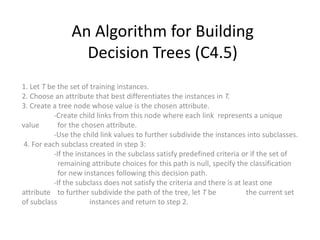
1. An Algorithm for Building Decision Trees (C4.5) 1. Let T be the set of training instances.2. Choose an attribute that best differentiates the instances in T.3. Create a tree node whose value is the chosen attribute. -Create child links from this node where each link represents a unique value for the chosen attribute. -Use the child link values to further subdivide the instances into subclasses. 4. For each subclass created in step 3: -If the instances in the subclass satisfy predefined criteria or if the set of remaining attribute choices for this path is null, specify the classification for new instances following this decision path. -If the subclass does not satisfy the criteria and there is at least one attribute to further subdivide the path of the tree, let T be the current set of subclass instances and return to step 2.

2. Entropy Example Given a set R of objects Entropy(R) = S (–p(I)log2p(I)) where p(I) is the proportion of set R that belongs to class I. An example: If set R is a collection of 14 objects, 9 of them belong to class A, and 5 of them belong to class B, then Entropy(R) = - (9/14) log2 (9/14) - (5/14) log2 (5/14) = 0.940 The range of entropy is from 0 (perfectly classified) to 1 (totally random).

3. Information Gain Example Actual example: Suppose there are 14 objects in set R, 9 of them belong to the class Evil, 5 of them belong to the class Good. Suppose that each object has an attribute Size, and Size can either be Big or Small. Suppose that out of these 14 objects, 8 have Size = Big, and 6 have Size = Small. Suppose that out of the 8 objects who have Size = Big, 6 are Evil and 2 are Good. Suppose that out of the 6 objects who have Size = Small, 3 are Evil and 3 are Good. Then, the information gain due to splitting R by attribute Size is: Gain(R,Size)=Entropy(R)-(8/14)*Entropy(RBig)-(6/14)*Entropy(RSmall) = 0.940 - (8/14)*0.811 - (6/14)*1.00 = 0.048 Entropy(RBig) = - (6/8)*log2(6/8) - (2/8)*log2(2/8) = 0.811 Entropy(RSmall) = - (3/6)*log2(3/6) - (3/6)*log2(3/6) = 1.00

4. Which attribute to use as split point for a node in decision tree? At the node, calculate information gain for each attribute. Choose the attribute that has the highest information gain, and use that as the split point. In the preceding example, the attribute Size has only two possible values. Often, an attribute can have more than two possible values, and we’d have to adapt the formula accordingly.

5. A Decision Tree Example The weather data example.

6. Information Gained by Knowing the Result of a Decision In the weather data example, there are 9 instances of which the decision to play is “yes” and there are 5 instances of which the decision to play is “no”. Then, the information gained by knowing the result of the decision is

7. Information Further Required If “Outlook” Is Placed at the Root Outlook sunny overcast rainy yes yes no no no yes yes yes yes yes yes yes no no

8. Information Gained by Placing Each of the 4 Attributes Gain(outlook) = 0.940 bits – 0.693 bits = 0.247 bits. Gain(temperature) = 0.029 bits. Gain(humidity) = 0.152 bits. Gain(windy) = 0.048 bits.

9. The Strategy for Selecting an Attribute to Place at a Node Select the attribute that gives us the largest information gain. In this example, it is the attribute “Outlook”. Outlook sunny overcast rainy 2 “yes” 3 “no” 4 “yes” 3 “yes” 2 “no”

10. The Recursive Procedure for Constructing a Decision Tree The operation discussed above is applied to each branch recursively to construct the decision tree. For example, for the branch “Outlook = Sunny”, we evaluate the information gained by applying each of the remaining 3 attributes. Gain(Outlook=sunny;Temperature) = 0.971 – 0.4 = 0.571 Gain(Outlook=sunny;Humidity) = 0.971 – 0 = 0.971 Gain(Outlook=sunny;Windy) = 0.971 – 0.951 = 0.02

11. Similarly, we also evaluate the information gained by applying each of the remaining 3 attributes for the branch “Outlook = rainy”. Gain(Outlook=rainy;Temperature) = 0.971 – 0.951 = 0.02 Gain(Outlook=rainy;Humidity) = 0.971 – 0.951 = 0.02 Gain(Outlook=rainy;Windy) =0.971 – 0 = 0.971

12. Over-fitting and Pruning If we recursively build the decision tree based on our training set until each leaf is totally classified, we have most likely over-fitted the data. To avoid over-fitting, we need to set aside part of the training data to test the decision tree, and prune (delete) the branches that give poor predictions.

13. The Over-fitting Issue Over-fitting is caused by creating decision rules that work accurately on the training set based on insufficient quantity of samples. As a result, these decision rules may not work well in more general cases.

15. Evaluation Training accuracy How many training instances can be correctly classify based on the available data? Is high when the tree is deep/large, or when there is less confliction in the training instances. however, higher training accuracy does not mean good generalization Testing accuracy Given a number of new instances, how many of them can we correctly classify? Cross validation

16. A partial decision tree with root node = income range

17. A partial decision tree with root node = credit card insurance

18. A three-node decision tree for the credit card database