The document introduces complex numbers and their properties. A complex number consists of a real part and an imaginary part. Complex numbers can be represented as vectors in a complex plane, with the real part as the x-axis and imaginary part as the y-axis. Operations such as addition, subtraction, multiplication and division of complex numbers are defined. Trigonometric functions are related to complex exponential functions. Solutions of quadratic equations with complex coefficients are also discussed.

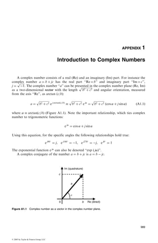
1. APPENDIX 1
Introduction to Complex Numbers
A complex number consists of a real (Re) and an imaginary (Im) part. For instance the
complex number a ¼ b þ jc has the real part ‘‘Re ¼ b’’ and imaginary part ‘‘Im ¼ c’’,
j ¼
ffiffiffiffiffiffiffi
À1
p
. The complex number ‘‘a’’ can be presented in the complex number plane (Re, Im)
as a two-dimensional vector with the length
ffiffiffiffiffiffiffiffiffiffiffiffiffiffiffi
b2 þ c2
p
and angular orientation, measured
from the axis ‘‘Re’’, as arctan (c/b):
a ¼
ffiffiffiffiffiffiffiffiffiffiffiffiffiffiffi
b2 þ c2
p
e j arctan c=bð Þ
ffiffiffiffiffiffiffiffiffiffiffiffiffiffiffi
b2 þ c2
p
e j
¼
ffiffiffiffiffiffiffiffiffiffiffiffiffiffiffi
b2 þ c2
p
cos þ j sin ð Þ ðA1:1Þ
where arctanðc=bÞ (Figure A1.1). Note the important relationship, which ties complex
number to trigonometric functions:
e j
¼ cos þ j sin
Using this equation, for the specific angles the following relationships hold true:
e j90
¼ j, e j180
¼ À1, e j270
¼ Àj, e j0
¼ 1
The exponential function e j
can also be denoted ‘‘exp ( j)’’.
A complex conjugate of the number a ¼ b þ jc is a ¼ b À jc.
Figure A1.1 Complex number as a vector in the complex number plane.
989
© 2005 by Taylor Francis Group, LLC

2. Note that in engineering use of complex numbers the imaginary part of the complex
number is often called ‘‘quadrature’’, in order to avoid connotations with ‘‘unreality’’. The
real part of the complex number is called ‘‘direct’’.
Using Eq. (A1.1), the relationship between trigonometric and exponential functions can
be derived as follows:
cos ¼
e j
þ eÀj
2
, sin ¼
e j
À eÀj
2j
¼ Àj
e j
À eÀj
2
The hyperbolic functions look somewhat similar to the above functions, but they do not
involve complex numbers in their exponential functions. The hyperbolic sine and cosine are
as follows:
sin h ¼
e
À eÀ
2
, cos h ¼
e
þ eÀ
2
The corresponding inverse functions are:
¼ arcsin hðAÞ ¼ ln A þ
ffiffiffiffiffiffiffiffiffiffiffiffiffiffi
A2 þ 1
p
, ¼ arccos hðAÞ ¼ ln A þ
ffiffiffiffiffiffiffiffiffiffiffiffiffiffi
A2 À 1
p
Similarly, the hyperbolic functions tangent and cotangent, and inverse functions arctan h,
arccotan h, are introduced.
The addition (subtraction) of two complex numbers, a1, a2 is as follows:
a1 þ a2 ¼ b1 þ jc1 Æ ðb2 þ jc2Þ ¼ ðb1 Æ b2Þ þ jðc1 Æ c2Þ
The addition (subtraction) of the complex numbers presented in the exponential format is
as follows:
A e j
Æ B e j

3. ¼ C e j
where
C ¼
ffiffiffiffiffiffiffiffiffiffiffiffiffiffiffiffiffiffiffiffiffiffiffiffiffiffiffiffiffiffiffiffiffiffiffiffiffiffiffiffiffiffiffiffiffiffiffiffiffiffiffiffiffiffi
A2 þ B2 Æ 2AB cosð À

4. Þ
p
,
¼ arctan
A sin Æ B sin

5. A cos Æ B cos

6. The multiplication of complex numbers is as follows:
a1a2 ¼ ðb1 þ jc1Þðb2 þ jc2Þ ¼ b1b2 À c1c2 þ jðb1c2 þ c1b2Þ
¼
ffiffiffiffiffiffiffiffiffiffiffiffiffiffiffi
b2
1 þ c2
1
q
e j arctanðc1=b1Þ
ffiffiffiffiffiffiffiffiffiffiffiffiffiffiffi
b2
2 þ c2
2
q
e j arctanðc2=b2Þ
¼
ffiffiffiffiffiffiffiffiffiffiffiffiffiffiffiffiffiffiffiffiffiffiffiffiffiffiffiffiffiffiffiffiffiffiffi
ðb2
1 þ c2
1Þðb2
2 þ c2
2Þ
q
e j arctanðc1=b1Þþarctanðc2=b2Þ½ Š
¼
ffiffiffiffiffiffiffiffiffiffiffiffiffiffiffiffiffiffiffiffiffiffiffiffiffiffiffiffiffiffiffiffiffiffiffi
ðb2
1 þ c2
1Þðb2
2 þ c2
2Þ
q
e j arctan ðb1c2þc1b2Þ=ðb1b2Àc1c2Þ½ Š
990 ROTORDYNAMICS
© 2005 by Taylor Francis Group, LLC

7. The division of complex numbers is as follows:
a1
a2
¼
b1 þ jc1
b2 þ jc2
¼
ðb1 þ jc1Þðb2 À jc2Þ
ðb2 þ jc2Þðb2 À jc2Þ
¼
b1b2 þ c1c2 þ jðc1b2 À b1c2Þ
b2
2 þ c2
2
¼
ffiffiffiffiffiffiffiffiffiffiffiffiffiffiffi
b2
1 þ c2
1
q
ffiffiffiffiffiffiffiffiffiffiffiffiffiffiffi
b2
2 þ c2
2
q e j arctanðc1=b1ÞÀarctanðc2=b2Þ½ Š
¼
ffiffiffiffiffiffiffiffiffiffiffiffiffiffiffi
b2
1 þ c2
1
q
ffiffiffiffiffiffiffiffiffiffiffiffiffiffiffi
b2
2 þ c2
2
q e j arctan ðc1b2Àb1c2Þ=ðb1b2þc1c2Þ½ Š
In the latter transformations the following trigonometric relationships were used (see also
arctan A Æ arctan B ¼ arctan C, where A ¼ c1=b1, B ¼ c2=b2
Æ

8. ¼
, where A ¼ tan , B ¼ tan

9. , C ¼ tan
tanð Æ

10. Þ ¼ tan
tan
¼
tan Æ tan

11. 1 Ç tan tan

12. ¼
A Æ B
1 Ç AB
C ¼ tan
¼
ðc1=b1Þ Æ ðc2=b2Þ
1 Ç ððc1c1Þ=ðb1b2ÞÞ
¼
c1b2 Æ b1c2
b1b2 Ç c1c2
A radical of a complex number is a complex number:
ffiffiffiffiffiffiffiffiffiffiffiffi
a þ jb
p
¼ c þ jd
a þ jb ¼ c2
þ 2jcd À d2
a ¼ c2
À d2
, b ¼ 2cd
From these real and imaginary parts, the unknown c and d can be calculated:
c2
À
b
2c
2
¼ a, c4
À ac2
À
b2
4
¼ 0
c ¼
ffiffiffiffiffiffiffiffiffiffiffiffiffiffiffiffiffiffiffiffiffiffiffiffiffiffiffiffiffiffiffiffiffiffiffiffi
1
2
a þ
ffiffiffiffiffiffiffiffiffiffiffiffiffiffiffi
a2 þ b2
p r
, d ¼
ffiffiffiffiffiffiffiffiffiffiffiffiffiffiffiffiffiffiffiffiffiffiffiffiffiffiffiffiffiffiffiffiffiffiffiffiffiffiffi
1
2
Àa þ
ffiffiffiffiffiffiffiffiffiffiffiffiffiffiffi
a2 þ b2
p r
Thus
ffiffiffiffiffiffiffiffiffiffiffiffi
a þ jb
p
¼
ffiffiffiffiffiffiffiffiffiffiffiffiffiffiffiffiffiffiffiffiffiffiffiffiffiffiffiffiffiffiffiffiffiffiffiffi
1
2
a þ
ffiffiffiffiffiffiffiffiffiffiffiffiffiffiffi
a2 þ b2
p r
þ j
ffiffiffiffiffiffiffiffiffiffiffiffiffiffiffiffiffiffiffiffiffiffiffiffiffiffiffiffiffiffiffiffiffiffiffiffiffiffiffi
1
2
Àa þ
ffiffiffiffiffiffiffiffiffiffiffiffiffiffiffi
a2 þ b2
p r
The solution of a quadratic equation with complex coefficients, such as the characteristic
equation of linear systems s2
þ ða þ jbÞs þ c þ jd ¼ 0 is as follows:
s ¼ À
a þ jb
2
Æ
ffiffiffiffiffiffiffiffiffiffiffiffiffiffiffiffiffiffiffiffiffiffiffiffiffiffiffiffiffiffiffiffiffiffiffiffi
a þ jb
2
2
Àc À jd
s
INTRODUCTION TO COMPLEX NUMBERS 991
© 2005 by Taylor Francis Group, LLC
Appendix 6):

13. and further, using the formulas developed above:
s ¼ À
a
2
Æ
1
ffiffiffi
2
p
ffiffiffiffiffiffiffiffiffiffiffiffiffiffiffiffiffiffiffiffiffiffiffiffiffiffiffiffiffiffiffiffiffiffiffiffiffiffiffiffiffiffiffiffiffiffiffiffiffiffiffiffiffiffiffiffiffiffiffiffiffiffiffiffiffiffiffiffiffiffiffiffiffiffiffiffiffiffiffiffiffiffiffiffiffiffiffiffi
a2 À b2
4
À c þ
ffiffiffiffiffiffiffiffiffiffiffiffiffiffiffiffiffiffiffiffiffiffiffiffiffiffiffiffiffiffiffiffiffiffiffiffiffiffiffiffiffiffiffiffiffiffiffiffiffiffiffiffiffiffiffiffi
a2 À b2
4
À c
2
þ
ab
2
À d
2
sv
u
u
t
2
6
4
3
7
5þ
À j
b
2
Æ
1
ffiffiffi
2
p
ffiffiffiffiffiffiffiffiffiffiffiffiffiffiffiffiffiffiffiffiffiffiffiffiffiffiffiffiffiffiffiffiffiffiffiffiffiffiffiffiffiffiffiffiffiffiffiffiffiffiffiffiffiffiffiffiffiffiffiffiffiffiffiffiffiffiffiffiffiffiffiffiffiffiffiffiffiffiffiffiffiffiffiffiffiffiffiffiffiffiffiffiffi
À
a2 À b2
4
þ c þ
ffiffiffiffiffiffiffiffiffiffiffiffiffiffiffiffiffiffiffiffiffiffiffiffiffiffiffiffiffiffiffiffiffiffiffiffiffiffiffiffiffiffiffiffiffiffiffiffiffiffiffiffiffiffiffiffi
a2 À b2
4
À c
2
þ
ab
2
À d
2
sv
u
u
t
2
6
4
3
7
5
8
:
9
=
;
There are four solutions resulting from four combinations of signs ‘Æ’ of the quadratic
equation with complex numbers. These four solutions are actually two pairs of complex
conjugate numbers.
In vibration measurements, the use of complex numbers in the representation of
measured amplitudes and phases of the vibration waveforms, filtered to specific frequencies,
makes data processing easier. The amplitude A and phase are presented in the form of a
complex vector, Ae j
. In industry, the formal representation of measured amplitudes and
phases are usually presented in the notation Aff (amplitude A at angle ) and for algebraic
transformations, the formulas are given following the above formal derivation. This is often
applied in the routines of the one- or two-plane balancing.
992 ROTORDYNAMICS
© 2005 by Taylor Francis Group, LLC