Multinomial logisticregression basicrelationships
•Download as PPT, PDF•
8 likes•4,098 views

Multinomial logistic regression

Recommended
More Related Content
What's hot
What's hot (20)
Viewers also liked
Similar to Multinomial logisticregression basicrelationships
Similar to Multinomial logisticregression basicrelationships (20)
Recently uploaded
Recently uploaded (20)
Multinomial logisticregression basicrelationships
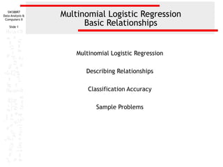
- 1. SW388R7 Data Analysis & Computers II Slide 1 Multinomial Logistic Regression Basic Relationships Multinomial Logistic Regression Describing Relationships Classification Accuracy Sample Problems
- 2. Compu ters II Multinomial logistic regression Slide 2 Multinomial logistic regression is used to analyze relationships between a non-metric dependent variable and metric or dichotomous independent variables. Multinomial logistic regression compares multiple groups through a combination of binary logistic regressions. The group comparisons are equivalent to the comparisons for a dummy-coded dependent variable, with the group with the highest numeric score used as the reference group. For example, if we wanted to study differences in BSW, MSW, and PhD students using multinomial logistic regression, the analysis would compare BSW students to PhD students and MSW students to PhD students. For each independent variable, there would be two comparisons.
- 3. Compu ters II What multinomial logistic regression predicts Slide 3 Multinomial logistic regression provides a set of coefficients for each of the two comparisons. The coefficients for the reference group are all zeros, similar to the coefficients for the reference group for a dummy-coded variable. Thus, there are three equations, one for each of the groups defined by the dependent variable. The three equations can be used to compute the probability that a subject is a member of each of the three groups. A case is predicted to belong to the group associated with the highest probability. Predicted group membership can be compared to actual group membership to obtain a measure of classification accuracy.
- 4. Compu ters II Level of measurement requirements Slide 4 Multinomial logistic regression analysis requires that the dependent variable be non-metric. Dichotomous, nominal, and ordinal variables satisfy the level of measurement requirement. Multinomial logistic regression analysis requires that the independent variables be metric or dichotomous. Since SPSS will automatically dummy-code nominal level variables, they can be included since they will be dichotomized in the analysis. In SPSS, non-metric independent variables are included as “factors.” SPSS will dummy-code non-metric IVs. In SPSS, metric independent variables are included as “covariates.” If an independent variable is ordinal, we will attach the usual caution.
- 5. Compu ters II Assumptions and outliers Slide 5 Multinomial logistic regression does not make any assumptions of normality, linearity, and homogeneity of variance for the independent variables. Because it does not impose these requirements, it is preferred to discriminant analysis when the data does not satisfy these assumptions. SPSS does not compute any diagnostic statistics for outliers. To evaluate outliers, the advice is to run multiple binary logistic regressions and use those results to test the exclusion of outliers or influential cases.
- 6. Compu ters II Sample size requirements Slide 6 The minimum number of cases per independent variable is 10, using a guideline provided by Hosmer and Lemeshow, authors of Applied Logistic Regression, one of the main resources for Logistic Regression. For preferred case-to-variable ratios, we will use 20 to 1.
- 7. Compu ters II Methods for including variables Slide 7 The only method for selecting independent variables in SPSS is simultaneous or direct entry.
- 8. Compu ters II Overall test of relationship - 1 Slide 8 The overall test of relationship among the independent variables and groups defined by the dependent is based on the reduction in the likelihood values for a model which does not contain any independent variables and the model that contains the independent variables. This difference in likelihood follows a chi-square distribution, and is referred to as the model chi-square. The significance test for the final model chi-square (after the independent variables have been added) is our statistical evidence of the presence of a relationship between the dependent variable and the combination of the independent variables.
- 9. Compu ters II Slide 9 Overall test of relationship - 2 Model Fitting Information Model Intercept Only Final -2 Log Likelihood 284.429 265.972 Chi-Square 18.457 df Sig. 6 .005 The presence of a relationship between the dependent variable and combination of independent variables is based on the statistical significance of the final model chi-square in the SPSS table titled "Model Fitting Information". In this analysis, the probability of the model chi-square (18.457) was 0.005, less than or equal to the level of significance of 0.05. The null hypothesis that there was no difference between the model without independent variables and the model with independent variables was rejected. The existence of a relationship between the independent variables and the dependent variable was supported.
- 10. ters II Strength of multinomial logistic regression relationship Slide 10 While multinomial logistic regression does compute correlation measures to estimate the strength of the relationship (pseudo R square measures, such as Nagelkerke's R²), these correlations measures do not really tell us much about the accuracy or errors associated with the model. A more useful measure to assess the utility of a multinomial logistic regression model is classification accuracy, which compares predicted group membership based on the logistic model to the actual, known group membership, which is the value for the dependent variable.
- 11. ters II Slide 11 Evaluating usefulness for logistic models The benchmark that we will use to characterize a multinomial logistic regression model as useful is a 25% improvement over the rate of accuracy achievable by chance alone. Even if the independent variables had no relationship to the groups defined by the dependent variable, we would still expect to be correct in our predictions of group membership some percentage of the time. This is referred to as by chance accuracy. The estimate of by chance accuracy that we will use is the proportional by chance accuracy rate, computed by summing the squared percentage of cases in each group. The only difference between by chance accuracy for binary logistic models and by chance accuracy for multinomial logistic models is the number of groups defined by the dependent variable.
- 12. ters II Slide 12 Computing by chance accuracy The percentage of cases in each group defined by the dependent variable is found in the ‘Case Processing Summary’ table. Case Processing Summary N HIGHWAYS AND BRIDGES Valid Missing Total Subpopulation 1 2 3 62 93 12 167 103 270 153a Marginal Percentage 37.1% 55.7% 7.2% 100.0% a. The dependent variable has only one value observed in 146 (95.4%) subpopulations. The proportional by chance accuracy rate was computed by calculating the proportion of cases for each group based on the number of cases in each group in the 'Case Processing Summary', and then squaring and summing the proportion of cases in each group (0.371² + 0.557² + 0.072² = 0.453). The proportional by chance accuracy criteria is 56.6% (1.25 x 45.3% = 56.6%).
- 13. ters II Slide 13 Comparing accuracy rates To characterize our model as useful, we compare the overall percentage accuracy rate produced by SPSS at the last step in which variables are entered to 25% more than the proportional by chance accuracy. (Note: SPSS does not compute a cross-validated accuracy rate for multinomial logistic regression .) Classification Predicted Observed 1 2 3 Overall Percentage 1 15 7 5 16.2% 2 47 86 7 83.8% 3 0 0 0 .0% The classification accuracy rate was 60.5% which was greater than or equal to the proportional by chance accuracy criteria of 56.6% (1.25 x 45.3% = 56.6%). The criteria for classification accuracy is satisfied in this example. Percent Correct 24.2% 92.5% .0% 60.5%
- 14. ters II Slide 14 Numerical problems The maximum likelihood method used to calculate multinomial logistic regression is an iterative fitting process that attempts to cycle through repetitions to find an answer. Sometimes, the method will break down and not be able to converge or find an answer. Sometimes the method will produce wildly improbable results, reporting that a one-unit change in an independent variable increases the odds of the modeled event by hundreds of thousands or millions. These implausible results can be produced by multicollinearity, categories of predictors having no cases or zero cells, and complete separation whereby the two groups are perfectly separated by the scores on one or more independent variables. The clue that we have numerical problems and should not interpret the results are standard errors for some independent variables that are larger than 2.0.
- 15. ters II Relationship of individual independent variables and the dependent variable Slide 15 There are two types of tests for individual independent variables: The likelihood ratio test evaluates the overall relationship between an independent variable and the dependent variable The Wald test evaluates whether or not the independent variable is statistically significant in differentiating between the two groups in each of the embedded binary logistic comparisons. If an independent variable has an overall relationship to the dependent variable, it might or might not be statistically significant in differentiating between pairs of groups defined by the dependent variable.
- 16. ters II Relationship of individual independent variables and the dependent variable Slide 16 The interpretation for an independent variable focuses on its ability to distinguish between pairs of groups and the contribution which it makes to changing the odds of being in one dependent variable group rather than the other. We should not interpret the significance of an independent variable’s role in distinguishing between pairs of groups unless the independent variable also has an overall relationship to the dependent variable in the likelihood ratio test. The interpretation of an independent variable’s role in differentiating dependent variable groups is the same as we used in binary logistic regression. The difference in multinomial logistic regression is that we can have multiple interpretations for an independent variable in relation to different pairs of groups.
- 17. ters II Relationship of individual independent variables and the dependent variable Slide 17 Parameter Estimates HIGHWAYS a AND BRIDGES 1 2 Intercept AGE EDUC CONLEGIS Intercept AGE EDUC CONLEGIS B 3.240 .019 .071 -1.373 3.639 .003 .172 -1.657 Std. Error 2.478 .020 .108 .620 2.456 .020 .110 .613 95% Confidence Interva Exp(B) SPSS identifies the comparisons Exp(B) it makes for Bound Upper B Wald df Sig. Lower groups defined by1the dependent variable in 1.709 .191 the table of ‘Parameter Estimates,’ 1.019 either .980 using .906 1 .341 the value codes or the value labels, depending .427 1 .514 1.073 on the options settings for pivot table labeling. .868 4.913 1 .027 .253 .075 The 2.195 reference category is .138 identified in the 1 footnote to the table. .017 1 .897 1.003 .963 In this analysis, two comparisons will be 2.463 1 .117 1.188 .958 made: 7.298 1 .007 .191 .057 a. The reference category is: 3. HIGHWAYS a AND BRIDGES TOO LITTLE ABOUT RIGHT Intercept AGE EDUC CONLEGIS Intercept AGE EDUC CONLEGIS •the TOO LITTLE group (coded 1, shaded blue) will be compared to the TOO MUCH Parameter Estimates group (coded 3, shaded purple) •the ABOUT RIGHT group (coded 2 , shaded orange)) will be compared to the TOO MUCH group (coded 3, shaded purple). Wald Std. Error df Sig. Exp(B) B 3.240 2.478 1.709 1 .191 The reference category plays the same role in .019 .020 .906 1 .341 multinomial logistic regression that it plays in .071 .108 .427 1 .514 the dummy-coding of a nominal variable: it is the category that4.913 would be coded with .027 zeros -1.373 .620 1 for all of the dummy-coded variables that all 3.639 2.456 2.195 1 .138 other categories are interpreted against. .003 .020 .017 1 .897 .172 .110 2.463 1 .117 -1.657 .613 7.298 1 .007 a. The reference category is: TOO MUCH. 1.019 1.073 .253 1.003 1.188 .191 95% C Lower B
- 18. ters II Relationship of individual independent variables and the dependent variable Slide 18 Likelihood Ratio Tests Effect Intercept AGE EDUC CONLEGIS -2 Log Likelihood of Reduced Model 268.323 268.625 270.395 275.194 Chi-Square 2.350 2.652 4.423 9.221 df 2 2 2 2 Sig. .309 .265 .110 .010 In this example, there is a statistically significant relationship between the independent variable CONLEGIS and the dependent variable. (0.010 < 0.05) The chi-square statistic is the difference in -2 log-likelihoods between the final model and a reduced model. The reduced model is Parameter Estimates formed by omitting an effect from the final model. The null hypothesis is that all parameters of that effect are 0. HIGHWAYS a AND BRIDGES 1 2 B 3.240 .019 .071 -1.373 3.639 .003 .172 -1.657 Intercept AGE EDUC CONLEGIS Intercept AGE EDUC CONLEGIS Std. Error 2.478 .020 .108 .620 2.456 .020 .110 .613 Wald 1.709 .906 .427 4.913 2.195 .017 2.463 7.298 df 1 1 1 1 1 1 1 1 As well, the independent variable CONLEGIS is significant in distinguishing both category 1 of 95% Confidence Interval f the dependent variable from Exp(B) category 3 of the dependent Sig. Exp(B) Lower variable. (0.027 < 0.05) Bound Upper Bou .191 .341 .514 .027 .138 .897 .117 .007 a. The reference category is: 3. And the independent variable CONLEGIS is significant in distinguishing category 2 of the dependent variable from category 3 of the dependent variable. (0.007 < 0.05) 1.019 1.073 .253 .980 .868 .075 1.0 1.3 .8 1.003 1.188 .191 .963 .958 .057 1.0 1.4 .6
- 19. ters II Interpreting relationship of individual independent variables to the dependent variable Slide 19 Likelihood Ratio Tests Effect Intercept AGE EDUC CONLEGIS -2 Log Survey Likelihood of respondents who had less confidence in congress (higher values correspond to lower confidence) were less likely to be in the Reduced group ofChi-Square survey respondents who thought we spend too little money Model df Sig. on highways and bridges (DV category 1), rather than the group of 268.323 respondents who thought we spend too much money on 2.350 2 .309 survey 268.625 2.652 .265 highways and bridges (DV 2 category 3). 270.395 4.423 2 .110 For each unit9.221 increase in confidence in Congress, the odds of being 275.194 2 .010 in the group of survey respondents who thought we spend too little The chi-square statistic is theon highwayslog-likelihoods decreased by 74.7%. (0.253 – 1.0 money difference in -2 and bridges between the final model-0.747) = and a reduced model. The reduced model is Parameter Estimates formed by omitting an effect from the final model. The null hypothesis is that all parameters of that effect are 0. HIGHWAYS a AND BRIDGES 1 2 Intercept AGE EDUC CONLEGIS Intercept AGE EDUC CONLEGIS a. The reference category is: 3. B 3.240 .019 .071 -1.373 3.639 .003 .172 -1.657 Std. Error 2.478 .020 .108 .620 2.456 .020 .110 .613 Wald 1.709 .906 .427 4.913 2.195 .017 2.463 7.298 df 1 1 1 1 1 1 1 1 Sig. .191 .341 .514 .027 .138 .897 .117 .007 Exp(B) 95% Confidence Interval f Exp(B) Lower Bound Upper Bou 1.019 1.073 .253 .980 .868 .075 1.0 1.3 .8 1.003 1.188 .191 .963 .958 .057 1.0 1.4 .6
- 20. ters II Interpreting relationship of individual independent variables to the dependent variable Slide 20 Likelihood Ratio Tests Effect Intercept AGE EDUC CONLEGIS -2 Log Likelihood of Reduced Model 268.323 268.625 270.395 275.194 Chi-Square 2.350 2.652 4.423 9.221 df 2 2 2 2 Sig. .309 .265 .110 .010 Survey respondents who had less confidence in congress (higher The chi-square statistic is the difference in -2 log-likelihoods confidence) were less likely to be in the values correspond to lower group of survey The reduced model is between the final model and a reduced model. respondents who thought we spend about the right Parameter Estimates amount of money The null hypothesis formed by omitting an effect from the final model.on highways and bridges (DV category 2), rather than the group of survey respondents who thought we spend too is that all parameters of that effect are 0. much money on highways and bridges (DV Category 3). HIGHWAYS a AND BRIDGES 1 2 B Std. Error Wald df Sig. Exp(B) For each unit increase in confidence in Congress, the odds of being in Intercept the group of survey respondents who thought we spend about the 3.240 2.478 1.709 1 .191 right amount of money on highways and bridges decreased by AGE .019 .020 1 .341 1.019 80.9%. (0.191 – 1.0 = 0.809) .906 EDUC .071 .108 .427 1 .514 1.073 CONLEGIS -1.373 .620 4.913 1 .027 .253 Intercept 3.639 2.456 2.195 1 .138 AGE .003 .020 .017 1 .897 1.003 EDUC .172 .110 2.463 1 .117 1.188 CONLEGIS -1.657 .613 7.298 1 .007 .191 a. The reference category is: 3. 95% Confidence Interval f Exp(B) Lower Bound Upper Bou .980 .868 .075 1.0 1.3 .8 .963 .958 .057 1.0 1.4 .6
- 21. ters II Relationship of individual independent variables and the dependent variable Slide 21 Likelihood Ratio Tests Effect Intercept AGE EDUC POLVIEWS SEX -2 Log Likelihood of Reduced Model 327.463a 333.440 329.606 334.636 338.985 Chi-Square .000 5.976 2.143 7.173 11.521 df Sig. 0 2 2 2 2 . .050 .343 .028 .003 The chi-square statistic is the difference in -2 log-likelihoods Parameter Estimates between the final model and a reduced model. The reduced model is formed by omitting an effect from the final model. The null hypothesis is that all parameters of that effect are 0. a. a NATCHLD B Std. Error Wald df This reduced model is equivalent to the final2.233 because model TOO LITTLE Intercept 8.434 14.261 1 omitting the effect does not increase the degrees of freedom. AGE -.023 .017 1.756 1 EDUC -.066 .102 .414 1 POLVIEWS -.575 .251 5.234 1 [SEX=1] -2.167 .805 7.242 1 b [SEX=2] 0 . . 0 ABOUT RIGHT Intercept 4.485 2.255 3.955 1 AGE -.001 .018 .003 1 EDUC .011 .104 .011 1 POLVIEWS -.397 .257 2.375 1 [SEX=1] -1.606 .824 3.800 1 b [SEX=2] 0 . . 0 a. The reference category is: TOO MUCH. In this example, there is a statistically significant relationship between SEX and the dependent variable, spending on childcare assistance. As well, SEX plays a statistically significant role in differentiating 95% Confidence Interval the TOO LITTLE group from the TOO Exp(B) MUCH Exp(B) (reference) group. Sig. Lower Bound Upper Bo (0.007 < 0.5) .000 .185 .977 .944 .520 .936 .766 .022 .563 .344 .007 .115 .024 . . . However, SEX does not .047differentiate the ABOUT .955RIGHT .999 .965 group from the TOO MUCH (reference) .916 1.011 .824 group.(0.51 > 0.5) .123 .673 .406 .051 .201 .040 . . . 1. 1. . . 1. 1. 1. 1.
- 22. ters II Slide 22 Interpreting relationship of individual independent variables and the dependent variable Likelihood Ratio Tests Effect Intercept AGE EDUC POLVIEWS SEX -2 Log Likelihood of Reduced Model Chi-Square df Sig. 327.463a .000 0 . Survey respondents who were2 male (code 1 for sex) were less likely 333.440 5.976 .050 to 329.606 be in the group of survey respondents who thought we spend too 2.143 2 .343 little money on childcare assistance (DV category 1), rather than the 334.636 2 .028 group of survey 7.173 respondents who thought we spend too much money on childcare assistance (DV category 3). 338.985 11.521 2 .003 The chi-square statistic is the difference in -2 log-likelihoods Survey respondents who were male were 88.5% less likely (0.115 – Parameter Estimates between the final model and a reduced model. The reduced model 1.0 = -0.885) to be in the group of survey respondents who thought is formed by omittingspend too little final model. The null we an effect from the money on childcare assistance. hypothesis is that all parameters of that effect are 0. a. a NATCHLD B Std. Error Wald df Sig. Exp(B) This reduced model is equivalent to the final2.233 because model TOO LITTLE Intercept 8.434 14.261 1 .000 omitting the effect does not increase the degrees of freedom. AGE -.023 .017 1.756 1 .185 .977 EDUC -.066 .102 .414 1 .520 .936 POLVIEWS -.575 .251 5.234 1 .022 .563 [SEX=1] -2.167 .805 7.242 1 .007 .115 b [SEX=2] 0 . . 0 . . ABOUT RIGHT Intercept 4.485 2.255 3.955 1 .047 AGE -.001 .018 .003 1 .955 .999 EDUC .011 .104 .011 1 .916 1.011 POLVIEWS -.397 .257 2.375 1 .123 .673 [SEX=1] -1.606 .824 3.800 1 .051 .201 b [SEX=2] 0 . . 0 . . a. The reference category is: TOO MUCH. 95% Confidence Interval Exp(B) Lower Bound Upper Bo .944 .766 .344 .024 . 1. 1. . . .965 .824 .406 .040 . 1. 1. 1. 1.
- 23. ters II Interpreting relationships for independent variable in problems Slide 23 In the multinomial logistic regression problems, the problem statement will ask about only one of the independent variables. The answer will be true or false based on only the relationship between the specified independent variable and the dependent variable. The individual relationships between other independent variables are the dependent variable are not used in determining whether or not the answer is true or false.
- 24. ters II Slide 24 Problem 1 11. In the dataset GSS2000, is the following statement true, false, or an incorrect application of a statistic? Assume that there is no problem with missing data, outliers, or influential cases, and that the validation analysis will confirm the generalizability of the results. Use a level of significance of 0.05 for evaluating the statistical relationships. The variables "age" [age], "highest year of school completed" [educ] and "confidence in Congress" [conlegis] were useful predictors for distinguishing between groups based on responses to "opinion about spending on highways and bridges" [natroad]. These predictors differentiate survey respondents who thought we spend too little money on highways and bridges from survey respondents who thought we spend too much money on highways and bridges and survey respondents who thought we spend about the right amount of money on highways and bridges from survey respondents who thought we spend too much money on highways and bridges. Among this set of predictors, confidence in Congress was helpful in distinguishing among the groups defined by responses to opinion about spending on highways and bridges. Survey respondents who had less confidence in congress were less likely to be in the group of survey respondents who thought we spend too little money on highways and bridges, rather than the group of survey respondents who thought we spend too much money on highways and bridges. For each unit increase in confidence in Congress, the odds of being in the group of survey respondents who thought we spend too little money on highways and bridges decreased by 74.7%. Survey respondents who had less confidence in congress were less likely to be in the group of survey respondents who thought we spend about the right amount of money on highways and bridges, rather than the group of survey respondents who thought we spend too much money on highways and bridges. For each unit increase in confidence in Congress, the odds of being in the group of survey respondents who thought we spend about the right amount of money on highways and bridges decreased by 80.9%. 1. 2. 3. 4. True True with caution False Inappropriate application of a statistic
- 25. ters II Slide 25 Dissecting problem 1 - 1 11. In the dataset GSS2000, is the following statement true, false, or an incorrect application of a statistic? Assume that there is no problem with missing data, outliers, or influential cases, and that the validation analysis will confirm the generalizability of the results. Use a level of significance of 0.05 for evaluating the statistical relationships. The variables "age" [age], "highest year of school completed" [educ] and "confidence in Congress" [conlegis] were useful predictors for distinguishing between groups based on responses to "opinion about spending on highways and bridges" [natroad]. These predictors differentiate survey respondents who For thesewe spend too little money on highways and thought problems, we will bridges from survey respondents who assume that spend is nomuch money on highways and thought we there too problem bridges and survey respondents who thought we spend about the right amount of money on with missing data, outliers, or highways and bridges from survey respondents who thought wethe influential cases, and that spend too much money on highways and bridges. validation analysis will confirm the generalizability of the Among this set of predictors, confidence in Congress was helpful in distinguishing among the results groups defined by responses to opinion about spending on highways and bridges. Survey respondents who had less confidence in congress were less likely to be in the group of survey In this money we are told and respondents who thought we spend too littleproblem,on highways to bridges, rather than the use we spend too much group of survey respondents who thought 0.05 as alpha for the money on highways and bridges. For each unit increase in confidence in Congress, logistic regression. in the group of survey multinomial the odds of being respondents who thought we spend too little money on highways and bridges decreased by 74.7%. Survey respondents who had less confidence in congress were less likely to be in the group of survey respondents who thought we spend about the right amount of money on highways and bridges, rather than the group of survey respondents who thought we spend too much money on highways and bridges. For each unit increase in confidence in Congress, the odds of being in the group of survey respondents who thought we spend about the right amount of money on highways and bridges decreased by 80.9%. 1. 2. 3. 4. True True with caution False Inappropriate application of a statistic
- 26. ters II Slide 26 Dissecting problem 1 - 2 The variables listed first in the problem statement are the independent variables (IVs): "age" [age], "highest year of school 11. In the dataset GSS2000,"confidence in completed" [educ] and is the following statement true, false, or an incorrect application of a statistic? Assume that there is no problem with missing data, outliers, or influential cases, Congress" [conlegis]. and that the validation analysis will confirm the generalizability of the results. Use a level of significance of 0.05 for evaluating the statistical relationships. The variables "age" [age], "highest year of school completed" [educ] and "confidence in Congress" [conlegis] were useful predictors for distinguishing between groups based on responses to "opinion about spending on highways and bridges" [natroad]. These predictors differentiate survey respondents who thought we spend too little money on highways and bridges from survey respondents who thought we spend too much money on highways and bridges and survey respondents who thought we spend about the right amount of money on highways and bridges from survey respondents who thought we spend too much money on The variable used to define highways and bridges.the dependent groups is variable (DV): "opinion about Among this set of predictors, confidence in Congress was helpful in distinguishing among the spending on highways and groups defined by responses to opinion about spending on highways and bridges. Survey respondents bridges" [natroad]. who had less confidence in congress were less likely to be in the group of survey respondents who thought we spend too little money on highways and bridges, rather than the group of survey respondents who thought we spend too much money on highways and bridges. For each unit increase in confidence in Congress, the odds of being in the group of survey respondents who thought we spend too little moneySPSS only supports direct or on highways and bridges decreased by simultaneous entry of independent in the 74.7%. Survey respondents who had less confidence in congress were less likely to be group of survey respondents who thought we spend variables in multinomial logistic about the right amount of money on regression, so we have no choice of highways and bridges, rather than the group of survey respondents who thought we spend too much money on highways and bridges. For each unitmethod for entering variables. increase in confidence in Congress, the odds of being in the group of survey respondents who thought we spend about the right amount of money on highways and bridges decreased by 80.9%.
- 27. ters II Slide 27 Dissecting problem 1 - 3 SPSS multinomial logistic regression models the relationship by comparing each of the groups defined by the dependent variable to the group with the highest code value. 11. In the dataset GSS2000, opinionfollowing statement true, false, or an incorrect application The responses to is the about spending on highways and bridges were: of a statistic? Assume that there is no problem with missing data, outliers, or influential cases, and that the validation analysis will confirm the= Too much. generalizability of the results. Use a level of 1= Too little, 2 = About right, and 3 significance of 0.05 for evaluating the statistical relationships. The variables "age" [age], "highest year of school completed" [educ] and "confidence in Congress" [conlegis] were useful predictors for distinguishing between groups based on responses to "opinion about spending on highways and bridges" [natroad]. These predictors differentiate survey respondents who thought we spend too little money on highways and bridges from survey respondents who thought we spend too much money on highways and bridges and survey respondents who thought we spend about the right amount of money on highways and bridges from survey respondents who thought we spend too much money on highways and bridges. Among this set of predictors, confidence in Congress was helpful in distinguishing among the groups defined by responses to opinion about spending on highways and bridges. Survey respondents who had less confidence in congress were less likely to be in the group of survey respondents who The analysis spend too in two money on highways and bridges, rather than the thought we will result little comparisons: group of survey respondents who thought we spend too spend too little money • survey respondents who thought we much money on highways and bridges. For each unit increase in confidence in Congress, the odds of being in the group of survey versus survey respondents who thought we spend too much respondents who thought we spend too and bridges on highways and bridges decreased by money on highways little money 74.7%. Survey respondents respondents who thought wecongress were less likely to be in the • survey who had less confidence in spend about the right group of survey respondentsof money versus survey respondents whoamount of money on who thought we spend about the right thought we amount highways and bridges, rather than the group of survey respondents who thought we spend too spend too bridges. For on highways and bridges. much money on highways and much money each unit increase in confidence in Congress, the odds of being in the group of survey respondents who thought we spend about the right amount of money on highways and bridges decreased by 80.9%.
- 28. ters II Slide 28 Dissecting problem 1 - 4 Each problem includes a statement about the relationship between one independent variable and the dependent variable. The answer to the problem is based on the stated relationship, ignoring the The variablesrelationships between the other independent variables and the "age" [age], "highest year of school completed" [educ] and "confidence in dependent variable. Congress" [conlegis] were useful predictors for distinguishing between groups based on responses to "opinion about spending on highways and bridges" [natroad]. These predictors differentiate This problem identifies a difference forspendof the comparisons highways and survey respondents who thought we both too little money on bridges from among respondents who thought we spend too much money on highways and survey groups modeled by the multinomial logistic regression. bridges and survey respondents who thought we spend about the right amount of money on highways and bridges from survey respondents who thought we spend too much money on highways and bridges. Among this set of predictors, confidence in Congress was helpful in distinguishing among the groups defined by responses to opinion about spending on highways and bridges. Survey respondents who had less confidence in congress were less likely to be in the group of survey respondents who thought we spend too little money on highways and bridges, rather than the group of survey respondents who thought we spend too much money on highways and bridges. For each unit increase in confidence in Congress, the odds of being in the group of survey respondents who thought we spend too little money on highways and bridges decreased by 74.7%. Survey respondents who had less confidence in congress were less likely to be in the group of survey respondents who thought we spend about the right amount of money on highways and bridges, rather than the group of survey respondents who thought we spend too much money on highways and bridges. For each unit increase in confidence in Congress, the odds of being in the group of survey respondents who thought we spend about the right amount of money on highways and bridges decreased by 80.9%.
- 29. ters II Slide 29 Dissecting problem 1 - 5 11. In the dataset GSS2000, is the following statement true, false, or an incorrect application of a statistic? Assume that there is no problem with missing data, outliers, or influential cases, and that the validation analysis will confirm the generalizability of the results. Use a level of significance of 0.05 for evaluating the statistical relationships. The variables "age" [age], "highest year of school completed" [educ] and "confidence in Congress" [conlegis] were useful predictors for distinguishing between groups based on responses to "opinion about spending on highways and bridges" [natroad]. These predictors differentiate survey respondents who thought we spend too little money on highways and bridges from survey respondents who thought we spend too much money on highways and bridges and survey respondents who thought we spend about the right amount of money on highways and bridges from survey respondents who thought we spend too much money on highways and bridges. Among this set of predictors, confidence in Congress was helpful in distinguishing among the groups defined by responses to opinion about spending on highways and bridges. Survey respondents who had less confidence in congress were less likely to be in the group of survey respondents who thought we spend too little money on highways and bridges, rather than the group of survey respondents who thought we spend too much money on highways and bridges. In order for the multinomial logistic regression For each unit increase in confidence in Congress, the odds of being in the group of survey question to be on highways and bridges decreased respondents who thought we spend too little money true, the overall relationship must by be statistically significant, were less be no 74.7%. Survey respondents who had less confidence in congress there mustlikely to be in the evidence of numerical problems, the classification group of survey respondents who thought we spend about the right amount of money on highways and bridges, rather than the accuracy rate must be substantiallythought we spend too group of survey respondents who better than much money on highways and bridges.couldeach unit increase in confidence in Congress, the For be obtained by chance alone, and the odds of being in the group of survey respondents who thought we spendbe statistically amount stated individual relationship must about the right of money on highways and bridges decreased by and interpreted correctly. significant 80.9%.
- 30. ters II Slide 30 Request multinomial logistic regression Select the Regression | Multinomial Logistic… command from the Analyze menu.
- 31. ters II Slide 31 Selecting the dependent variable First, highlight the dependent variable natroad in the list of variables. Second, click on the right arrow button to move the dependent variable to the Dependent text box.
- 32. ters II Slide 32 Selecting metric independent variables Metric independent variables are specified as covariates in multinomial logistic regression. Metric variables can be either interval or, by convention, ordinal. Move the metric independent variables, age, educ and conlegis to the Covariate(s) list box. In this analysis, there are no nonmetric independent variables. Nonmetric independent variables would be moved to the Factor(s) list box.
- 33. ters II Slide 33 Specifying statistics to include in the output While we will accept most of the SPSS defaults for the analysis, we need to specifically request the classification table. Click on the Statistics… button to make a request.
- 34. ters II Slide 34 Requesting the classification table First, keep the SPSS defaults for Summary statistics, Likelihood ratio test, and Parameter estimates. Second, mark the checkbox for the Classification table. Third, click on the Continue button to complete the request.
- 35. ters II Slide 35 Completing the multinomial logistic regression request Click on the OK button to request the output for the multinomial logistic regression. The multinomial logistic procedure supports additional commands to specify the model computed for the relationships (we will use the default main effects model), additional specifications for computing the regression, and saving classification results. We will not make use of these options.
- 36. ters II Slide 36 LEVEL OF MEASUREMENT - 1 11. In the dataset GSS2000, is the following statement true, false, or an incorrect application of a statistic? Assume that there is no problem with missing data, outliers, or influential cases, and that the validation analysis will confirm the generalizability of the results. Use a level of significance of 0.05 for evaluating the statistical relationships. The variables "age" [age], "highest year of school completed" [educ] and "confidence in Congress" [conlegis] were useful predictors for distinguishing between groups based on responses to "opinion about spending on highways and bridges" [natroad]. These predictors differentiate survey respondents who thought we spend too little money on highways and bridges from survey respondents who thought we spend too much money on highways and bridges and survey respondents who thought we spend about the right amount of money on highways and bridges from survey respondents who thought we spend too much money on highways and bridges. Among this set of predictors, confidence in Congress was helpful in distinguishing among the groups defined by responses to opinion about spending on highways and bridges. Survey respondents who had less confidence in congressrequires that the to be in the group of survey Multinomial logistic regression were less likely respondents who thought we spend too little money andhighways and bridges, rather than the dependent variable be non-metric on the group of survey respondents who thought we spend too much money on highways and bridges. independent variables be metric or dichotomous. For each unit increase in confidence in Congress, the odds of being in the group of survey respondents who thought we spend too little money on highways and bridges decreased by "Opinion about spending on highways and bridges" [natroad] is confidence in congress were less likely to be in the 74.7%. Survey respondents who had lessordinal, satisfying the nonmetric level of thought we spend about the the group of survey respondents who measurement requirement forright amount of money on dependent variable. highways and bridges, rather than the group of survey respondents who thought we spend too much money on highways and bridges. For each unit increase in confidence in Congress, the It contains three respondents who thought we odds of being in the group of surveycategories: survey respondents spend about the right amount who thought we spend too of money on highways and bridges decreased little money, about the right amount of money, by 80.9%. and too much money on highways and bridges. 1. True 2. True with caution
- 37. ters II Slide 37 LEVEL OF MEASUREMENT - 2 "Age" [age] and "highest year of school completed" [educ] are interval, 11. satisfying the metric or dichotomous In the dataset GSS2000, is the following statement true, false, or an incorrect application of alevel of measurement requirement for statistic? Assume that there is no problem with missing data, outliers, or influential cases, independent variables. and that the validation analysis will confirm the generalizability of the results. Use a level of significance of 0.05 for evaluating the statistical relationships. The variables "age" [age], "highest year of school completed" [educ] and "confidence in Congress" [conlegis] were useful predictors for distinguishing between groups based on responses to "opinion about spending on highways and bridges" [natroad]. These predictors differentiate survey respondents who thought we spend too little money on highways and bridges from survey respondents who thought we spend too much money on highways and bridges and survey respondents who thought we spend about the right amount of money on highways and bridges from survey respondents who thought we spend too much money on "Confidence in Congress" [conlegis] is ordinal, highways and bridges. satisfying the metric or dichotomous level of measurement requirement for independent variables. If we follow the convention of treating Among this set of predictors, confidence in Congress was helpfulthe distinguishing among the ordinal level variables as metric variables, in level groups defined by responses to opinion about spending on highways is bridges. Survey of measurement requirement for the analysis and respondents who had less confidence in congress analysts do not agree in the group of survey satisfied. Since some data were less likely to be with this convention, a note of caution should be respondents who thought we spend too little money on highways and bridges, rather than the included in our interpretation. group of survey respondents who thought we spend too much money on highways and bridges. For each unit increase in confidence in Congress, the odds of being in the group of survey respondents who thought we spend too little money on highways and bridges decreased by 74.7%. Survey respondents who had less confidence in congress were less likely to be in the group of survey respondents who thought we spend about the right amount of money on highways and bridges, rather than the group of survey respondents who thought we spend too much money on highways and bridges. For each unit increase in confidence in Congress, the odds of being in the group of survey respondents who thought we spend about the right amount of money on highways and bridges decreased by 80.9%.
- 38. ters II Slide 38 Sample size – ratio of cases to variables Case Processing Summary N HIGHWAYS AND BRIDGES Valid Missing Total Subpopulation 1 2 3 62 93 12 167 103 270 153a Marginal Percentage 37.1% 55.7% 7.2% 100.0% a. The dependent variable has only one value observed Multinomial logistic regression requires that the minimum ratio in 146 (95.4%) subpopulations. of valid cases to independent variables be at least 10 to 1. The ratio of valid cases (167) to number of independent variables (3) was 55.7 to 1, which was equal to or greater than the minimum ratio. The requirement for a minimum ratio of cases to independent variables was satisfied. The preferred ratio of valid cases to independent variables is 20 to 1. The ratio of 55.7 to 1 was equal to or greater than the preferred ratio. The preferred ratio of cases to independent variables was satisfied.
- 39. ters II Slide 39 OVERALL RELATIONSHIP BETWEEN INDEPENDENT AND DEPENDENT VARIABLES Model Fitting Information Model Intercept Only Final -2 Log Likelihood 284.429 265.972 Chi-Square 18.457 df Sig. 6 .005 The presence of a relationship between the dependent variable and combination of independent variables is based on the statistical significance of the final model chi-square in the SPSS table titled "Model Fitting Information". In this analysis, the probability of the model chi-square (18.457) was 0.005, less than or equal to the level of significance of 0.05. The null hypothesis that there was no difference between the model without independent variables and the model with independent variables was rejected. The existence of a relationship between the independent variables and the dependent variable was supported.
- 40. ters II Slide 40 NUMERICAL PROBLEMS Parameter Estimates HIGHWAYS a AND BRIDGES 1 2 Intercept AGE EDUC CONLEGIS Intercept AGE EDUC CONLEGIS a. The reference category is: 3. B 3.240 .019 .071 -1.373 3.639 .003 .172 -1.657 Std. Error 2.478 .020 .108 .620 2.456 .020 .110 .613 Wald 1.709 .906 .427 4.913 2.195 .017 2.463 7.298 95% Confidence Inter Exp(B) Multicollinearity in the multinomial df Sig. Exp(B) logistic regression solution is Lower Bound Upper 1 by examining the standard .191 detected errors1for the .341 b coefficients. A 1.019 .980 standard error larger than 2.0 1 .514 1.073 .868 indicates numerical problems, such 1 .027 .253 .075 as multicollinearity among the 1 .138 independent variables, zero cells for a dummy-coded independent 1 .897 1.003 .963 variable because all of the subjects 1 .117 1.188 .958 have the same value for the 1 .007 .191 variable, and 'complete separation' .057 whereby the two groups in the dependent event variable can be perfectly separated by scores on one of the independent variables. Analyses that indicate numerical problems should not be interpreted. None of the independent variables in this analysis had a standard error larger than 2.0. (We are not interested in the standard errors associated with the intercept.)
- 41. ters II Slide 41 RELATIONSHIP OF INDIVIDUAL INDEPENDENT VARIABLES TO DEPENDENT VARIABLE - 1 Likelihood Ratio Tests Effect Intercept AGE EDUC CONLEGIS -2 Log Likelihood of Reduced Model 268.323 268.625 270.395 275.194 Chi-Square 2.350 2.652 4.423 9.221 df 2 2 2 2 Sig. .309 .265 .110 .010 The chi-square statistic is the difference in -2 log-likelihoods between the final model and a reduced model. The reduced model is formed by omitting an effect from the final model. The null hypothesis is that all parameters of that effect are 0. The statistical significance of the relationship between confidence in Congress and opinion about spending on highways and bridges is based on the statistical significance of the chi-square statistic in the SPSS table titled "Likelihood Ratio Tests". For this relationship, the probability of the chi-square statistic (9.221) was 0.010, less than or equal to the level of significance of 0.05. The null hypothesis that all of the b coefficients associated with confidence in Congress were equal to zero was rejected. The existence of a relationship between confidence in Congress and opinion about spending on highways and bridges was supported.
- 42. ters II RELATIONSHIP OF INDIVIDUAL INDEPENDENT VARIABLES TO DEPENDENT VARIABLE - 2 Slide 42 Parameter Estimates HIGHWAYS a AND BRIDGES 1 2 Intercept AGE EDUC CONLEGIS Intercept AGE EDUC CONLEGIS B 3.240 .019 .071 -1.373 3.639 .003 .172 -1.657 Std. Error 2.478 .020 .108 .620 2.456 .020 .110 .613 Wald 1.709 .906 .427 4.913 2.195 .017 2.463 7.298 df 1 1 1 1 1 1 1 1 Sig. .191 .341 .514 .027 .138 .897 .117 .007 a. The reference category is: 3. In the comparison of survey respondents who thought we spend too little money on highways and bridges to survey respondents who thought we spend too much money on highways and bridges, the probability of the Wald statistic (4.913) for the variable confidence in Congress [conlegis] was 0.027. Since the probability was less than or equal to the level of significance of 0.05, the null hypothesis that the b coefficient for confidence in Congress was equal to zero for this comparison was rejected. Exp(B) 95% Confiden Exp Lower Bound 1.019 1.073 .253 .980 .868 .075 1.003 1.188 .191 .963 .958 .057
- 43. ters II RELATIONSHIP OF INDIVIDUAL INDEPENDENT VARIABLES TO DEPENDENT VARIABLE - 3 Slide 43 Parameter Estimates HIGHWAYS a AND BRIDGES 1 2 Intercept AGE EDUC CONLEGIS Intercept AGE EDUC CONLEGIS B 3.240 .019 .071 -1.373 3.639 .003 .172 -1.657 Std. Error 2.478 .020 .108 .620 2.456 .020 .110 .613 Wald 1.709 .906 .427 4.913 2.195 .017 2.463 7.298 df 1 1 1 1 1 1 1 1 Sig. .191 .341 .514 .027 .138 .897 .117 .007 a. The reference category is: 3. The value of Exp(B) was 0.253 which implies that for each unit increase in confidence in Congress the odds decreased by 74.7% (0.253 - 1.0 = -0.747). The relationship stated in the problem is supported. Survey respondents who had less confidence in congress were less likely to be in the group of survey respondents who thought we spend too little money on highways and bridges, rather than the group of survey respondents who thought we spend too much money on highways and bridges. For each unit increase in confidence in Congress, the odds of being in the group of survey respondents who thought we spend too little money on highways and bridges decreased by 74.7%. Exp(B) 95% Confiden Exp Lower Bound 1.019 1.073 .253 .980 .868 .075 1.003 1.188 .191 .963 .958 .057
- 44. ters II RELATIONSHIP OF INDIVIDUAL INDEPENDENT VARIABLES TO DEPENDENT VARIABLE - 4 Slide 44 Parameter Estimates HIGHWAYS a AND BRIDGES 1 2 Intercept AGE EDUC CONLEGIS Intercept AGE EDUC CONLEGIS B 3.240 .019 .071 -1.373 3.639 .003 .172 -1.657 Std. Error 2.478 .020 .108 .620 2.456 .020 .110 .613 Wald 1.709 .906 .427 4.913 2.195 .017 2.463 7.298 df 1 1 1 1 1 1 1 1 Sig. .191 .341 .514 .027 .138 .897 .117 .007 a. The reference category is: 3. In the comparison of survey respondents who thought we spend about the right amount of money on highways and bridges to survey respondents who thought we spend too much money on highways and bridges, the probability of the Wald statistic (7.298) for the variable confidence in Congress [conlegis] was 0.007. Since the probability was less than or equal to the level of significance of 0.05, the null hypothesis that the b coefficient for confidence in Congress was equal to zero for this comparison was rejected. Exp(B) 95% Confiden Exp Lower Bound 1.019 1.073 .253 .980 .868 .075 1.003 1.188 .191 .963 .958 .057
- 45. ters II Slide 45 RELATIONSHIP OF INDIVIDUAL INDEPENDENT VARIABLES TO DEPENDENT VARIABLE - 5 Parameter Estimates 95% Con HIGHWAYS a AND BRIDGES 1 2 Intercept AGE EDUC CONLEGIS Intercept AGE EDUC CONLEGIS B 3.240 .019 .071 -1.373 3.639 .003 .172 -1.657 Std. Error 2.478 .020 .108 .620 2.456 .020 .110 .613 Wald 1.709 .906 .427 4.913 2.195 .017 2.463 7.298 df 1 1 1 1 1 1 1 1 Sig. .191 .341 .514 .027 .138 .897 .117 .007 a. The reference category is: 3. The value of Exp(B) was 0.191 which implies that for each unit increase in confidence in Congress the odds decreased by 80.9% (0.191-1.0=-0.809). The relationship stated in the problem is supported. Survey respondents who had less confidence in congress were less likely to be in the group of survey respondents who thought we spend about the right amount of money on highways and bridges, rather than the group of survey respondents who thought we spend too much money on highways and bridges. For each unit increase in confidence in Congress, the odds of being in the group of survey respondents who thought we spend about the right amount of money on highways and bridges decreased by 80.9%. Exp(B) Lower Bou 1.019 1.073 .253 .9 .8 .0 1.003 1.188 .191 .9 .9 .0
- 46. ters II Slide 46 CLASSIFICATION USING THE MULTINOMIAL LOGISTIC REGRESSION MODEL: BY CHANCE ACCURACY RATE The independent variables could be characterized as useful predictors distinguishing survey respondents who thought we spend too little money on highways and bridges, survey respondents who thought we spend about the right amount of money on highways and bridges and survey respondents who thought we spend too much money on highways and bridges if the classification accuracy rate was substantially higher than the accuracy attainable by chance alone. Operationally, the classification accuracy rate should be 25% or more higher than the proportional by chance accuracy rate. Case Processing Summary N HIGHWAYS AND BRIDGES 1 2 3 Marginal Percentage 37.1% 55.7% 7.2% 100.0% 62 93 12 Valid 167 Missing 103 Total 270 The proportional by chance accuracy rate was computed by Subpopulation 153 calculating the proportion of cases for eachagroup based on the number of cases in each group in the 'Case Processing a. Summary',The dependent variable has only one value the proportion of and then squaring and summing observed in 146 (95.4%) subpopulations. cases in each group (0.371² + 0.557² + 0.072² = 0.453).
- 47. ters II Slide 47 CLASSIFICATION USING THE MULTINOMIAL LOGISTIC REGRESSION MODEL: CLASSIFICATION ACCURACY Classification Predicted Observed 1 2 3 Overall Percentage 1 15 7 5 16.2% 2 47 86 7 83.8% 3 0 0 0 .0% The classification accuracy rate was 60.5% which was greater than or equal to the proportional by chance accuracy criteria of 56.6% (1.25 x 45.3% = 56.6%). The criteria for classification accuracy is satisfied. Percent Correct 24.2% 92.5% .0% 60.5%
- 48. ters II Slide 48 Answering the question in problem 1 - 1 11. In the dataset GSS2000, is the following statement true, false, or an incorrect application of a statistic? Assume that there is no problem with missing data, outliers, or influential cases, and that the validation analysis will confirm the generalizability of the results. Use a level of significance of 0.05 for evaluating the statistical relationships. The variables "age" [age], "highest year of school completed" [educ] and "confidence in Congress" [conlegis] were useful predictors for distinguishing between groups based on responses to "opinion about spending on highways and bridges" [natroad]. These predictors differentiate survey respondents who thought we spend too little money on highways and bridges from survey respondents who thought we spend too much money on highways and bridges and survey respondents who thought we spend about the right amount of money on highways and bridges from survey respondents who thought we spend too much money on highways and bridges. Among this set of predictors, confidence in Congress was helpful in distinguishing among the groups defined by responses to opinion about spending on highways and bridges. Survey We found a statistically significant be in respondents who had less confidence in congress were less likely tooverallthe group of survey relationship between highways and bridges, rather than the respondents who thought we spend too little money onthe combination of independent variables and the dependent group of survey respondents who thought we spend too much money on highways and bridges. variable. For each unit increase in confidence in Congress, the odds of being in the group of survey respondents who thought we spend too little money on highways and bridges decreased by 74.7%. Survey respondents who had less was no evidence of numerical less likelyin be in the There confidence in congress were problems to group of survey respondents who thought we spend about the right amount of money on the solution. highways and bridges, rather than the group of survey respondents who thought we spend too much money on highways and bridges. For each unit increaseaccuracy surpassed Moreover, the classification in confidence in Congress, the odds of being in the group of survey respondents whochance accuracy criteria, the right amount the proportional by thought we spend about of money on highways and bridges supporting the 80.9%.of the model. decreased by utility 1. True 2. True with caution 3. False
- 49. ters II Slide 49 Answering the question in problem 1 - 2 We verified that each statement about the [educ] and The variables "age" [age], "highest year of school completed" relationship "confidence in Congress" [conlegis]between an independent for distinguishingdependent groups based on were useful predictors variable and the between variable was correct in both direction of the relationship These predictors responses to "opinion about spending on highways and bridges" [natroad]. differentiate surveyand the change in likelihoodwe spend too little money on highways and respondents who thought associated with a one-unit bridges from survey change of the who thought variable, for both of the respondents independent we spend too much money on highways and bridges and survey respondents who thought we stated in the problem. amount of money on comparisons between groups spend about the right highways and bridges from survey respondents who thought we spend too much money on highways and bridges. Among this set of predictors, confidence in Congress was helpful in distinguishing among the groups defined by responses to opinion about spending on highways and bridges. Survey respondents who had less confidence in congress were less likely to be in the group of survey respondents who thought we spend too little money on highways and bridges, rather than the group of survey respondents who thought we spend too much money on highways and bridges. For each unit increase in confidence in Congress, the odds of being in the group of survey respondents who thought we spend too little money on highways and bridges decreased by 74.7%. Survey respondents who had less confidence in congress were less likely to be in the group of survey respondents who thought we spend about the right amount of money on highways and bridges, rather than the group of survey respondents who thought we spend too much money on highways and bridges. For each unit increase in confidence in Congress, the odds of being in the group of survey respondents who thought we spend about the right amount of money on highways and bridges decreased by 80.9%. 1. 2. 3. 4. True True with caution False Inappropriate application of a statistic The answer to the question is true with caution. A caution is added because of the inclusion of ordinal level variables.
- 50. ters II Slide 50 Problem 2 1. In the dataset GSS2000, is the following statement true, false, or an incorrect application of a statistic? Assume that there is no problem with missing data, outliers, or influential cases, and that the validation analysis will confirm the generalizability of the results. Use a level of significance of 0.05 for evaluating the statistical relationships. The variables "highest year of school completed" [educ], "sex" [sex] and "total family income" [income98] were useful predictors for distinguishing between groups based on responses to "opinion about spending on space exploration" [natspac]. These predictors differentiate survey respondents who thought we spend too little money on space exploration from survey respondents who thought we spend too much money on space exploration and survey respondents who thought we spend about the right amount of money on space exploration from survey respondents who thought we spend too much money on space exploration. Among this set of predictors, total family income was helpful in distinguishing among the groups defined by responses to opinion about spending on space exploration. Survey respondents who had higher total family incomes were more likely to be in the group of survey respondents who thought we spend about the right amount of money on space exploration, rather than the group of survey respondents who thought we spend too much money on space exploration. For each unit increase in total family income, the odds of being in the group of survey respondents who thought we spend about the right amount of money on space exploration increased by 6.0%. 1. 2. 3. 4. True True with caution False Inappropriate application of a statistic
- 51. ters II Slide 51 Dissecting problem 2 - 1 1. In the dataset GSS2000, is the following statement true, false, or an incorrect application of a statistic? Assume that there is no problem with missing data, outliers, or influential cases, and that the validation analysis will confirm the generalizability of the results. Use a level of significance of 0.05 for evaluating the statistical relationships. The variables "highest year of school completed" [educ], "sex" [sex] and "total family income" [income98] were useful predictors for distinguishing between groups based on responses to "opinion about spending on space exploration" [natspac]. we will predictors differentiate survey For these problems, These respondents who thought we spend too little money on is no problem assume that there space exploration from survey respondents who thought we spend too much money on outliers, or with missing data, space exploration and survey respondents who thought we spend about the right amount of money on space exploration from influential cases, and that the survey respondents who thought we spend too much moneyconfirm exploration. on space validation analysis will the generalizability of the Among this set of predictors, total family income was helpful in distinguishing among the results groups defined by responses to opinion about spending on space exploration. Survey respondents who had higher total familythis problem, we are told to to be in the group of survey In incomes were more likely respondents who thought we spend about0.05 right amount of money on space exploration, use the as alpha for the rather than the group of survey respondents who logistic regression. too much money on space multinomial thought we spend exploration. For each unit increase in total family income, the odds of being in the group of survey respondents who thought we spend about the right amount of money on space exploration increased by 6.0%. 1. 2. 3. 4. True True with caution False Inappropriate application of a statistic
- 52. ters II Slide 52 Dissecting problem 2 - 2 The variables listed first in the problem statement are the independent variables 1. In (IVs): "highest year of is the following statement true, false, or an incorrect application of the dataset GSS2000, school completed" a statistic? Assume [sex] there is nofamily [educ], "sex" that and "total problem with missing data, outliers, or influential cases, and that the validation analysis will confirm the generalizability of the results. Use a level of income" [income98]. significance of 0.05 for evaluating the statistical relationships. The variables "highest year of school completed" [educ], "sex" [sex] and "total family income" [income98] were useful predictors for distinguishing between groups based on responses to "opinion about spending on space exploration" [natspac]. These predictors differentiate survey respondents who thought we spend too little money on space exploration from survey respondents who thought we spend too much money on space exploration and survey respondents who thought we spend about the right amount of money on space exploration from survey respondents who thought we spend too much money on space The variable exploration. used to define groups is the dependent variable (DV): "opinion about Among this on space spending set of predictors, total family income was helpful in distinguishing among the groups defined by responses to opinion about spending on space exploration. Survey exploration" [natspac]. respondents who had higher total family incomes were more likely to be in the group of survey respondents who thought we spend about the right amount of money on space exploration, rather than the group of survey respondents who thought we spend too much money on space SPSS only odds of direct in exploration. For each unit increase in total family income, thesupports being or the group of simultaneous entry of independent survey respondents who thought we spend about the right amount of money on space variables in multinomial logistic exploration increased by 6.0%. 1. True 2. True with caution 3. False regression, so we have no choice of method for entering variables.
- 53. ters II Slide 53 Dissecting problem 2 - 3 SPSS multinomial logistic regression models the relationship by comparing each of the groups defined by the dependent variable to the group with the highest code value. 1. In the dataset GSS2000,to opinion about spending ontrue, false, or an incorrect application of The responses is the following statement the space a statistic? Assume that there is no problem with missing data, outliers, or influential cases, program were: and that the1= Too little, 2 = About right, and 3 = Too much. validation analysis will confirm the generalizability of the results. Use a level of significance of 0.05 for evaluating the statistical relationships. The variables "highest year of school completed" [educ], "sex" [sex] and "total family income" [income98] were useful predictors for distinguishing between groups based on responses to "opinion about spending on space exploration" [natspac]. These predictors differentiate survey respondents who thought we spend too little money on space exploration from survey respondents who thought we spend too much money on space exploration and survey respondents who thought we spend about the right amount of money on space exploration from survey respondents who thought we spend too much money on space exploration. Among this set of predictors, total family income was helpful in distinguishing among the The analysis will result about spending on groups defined by responses to opinion in two comparisons:space exploration. Survey respondents who • survey respondents who thought we spend likely to be in the group of survey had higher total family incomes were more too little money versus survey respondents who amount of money on space respondents who thought we spend about the rightthought we spend too much exploration, money on space exploration rather than the group of survey respondents who thought we spend too much money on space • survey increase in total family income, the odds the being in the group of exploration. For each unit respondents who thought we spend about of right amount of money versus survey respondents who money on survey respondents who thought we spend about the right amount ofthought we space exploration increased by 6.0%. spend too much money on space exploration. 1. True
- 54. ters II Slide 54 Dissecting problem 2 - 4 Each problem includes a statement about the The variables "highest year of school completed" [educ], "sex" [sex] and "total family income" [income98]relationship between onefor distinguishing between groups based on responses to were useful predictors independent variable and the dependenton space exploration" [natspac]. These predictors differentiate survey "opinion about spending variable. The answer to the problem is based on the stated relationship, respondents who thought we spend too little money on space exploration from survey respondents who thought we spend too much money on space exploration and survey ignoring the relationships between the other respondents who thought we spend about the right variable. of money on space exploration from independent variables and the dependent amount survey respondents who thought we spend too much money on space exploration. Among this set of predictors, total family income was helpful in distinguishing among the groups defined by responses to opinion about spending on space exploration. Survey respondents who had higher total family incomes were more likely to be in the group of survey respondents who thought we spend about the right amount of money on space exploration, rather than the group of survey respondents who thought we spend too much money on space exploration. For each unit increase in total family income, the odds of being in the group of survey respondents who thought we spend about the right amount of money on space exploration increased by 6.0%. 1. 2. 3. 4. True True with caution This problem identifies a difference for only one of the two comparisons based on the three values False Inappropriate application of a of the dependent variable. statistic Other problems will specify both of the possible comparisons.
- 55. ters II Slide 55 Dissecting problem 2 - 5 The variables "highest year of school completed" [educ], "sex" [sex] and "total family income" [income98] were useful predictors for distinguishing between groups based on responses to "opinion about spending on space exploration" [natspac]. These predictors differentiate survey respondents who thought we spend too little money on space exploration from survey respondents who thought we spend too much money on space exploration and survey respondents who thought we spend about the right amount of money on space exploration from survey respondents who thought we spend too much money on space exploration. Among this set of predictors, total family income was helpful in distinguishing among the groups defined by responses to opinion about spending on space exploration. Survey respondents who had higher total family incomes were more likely to be in the group of survey respondents who thought we spend about the right amount of money on space exploration, rather than the group of survey respondents who thought we spend too much money on space exploration. For each unit increase in total family income, the odds of being in the group of survey respondents who thought we spend about the right amount of money on space exploration increased by 6.0%. 1. 2. 3. 4. True In order for the multinomial logistic regression question to be true, the overall relationship must True with caution be statistically significant, there must be no False evidence of numerical problems, the classification Inappropriate application of a statistic accuracy rate must be substantially better than could be obtained by chance alone, and the stated individual relationship must be statistically significant and interpreted correctly.
- 56. ters II Slide 56 LEVEL OF MEASUREMENT - 1 1. In the dataset GSS2000, is the following statement true, false, or an incorrect application of a statistic? Assume that there is no problem with missing data, outliers, or influential cases, and that the validation analysis will confirm the generalizability of the results. Use a level of significance of 0.05 for evaluating the statistical relationships. The variables "highest year of school completed" [educ], "sex" [sex] and "total family income" [income98] were useful predictors for distinguishing between groups based on responses to "opinion about spending on space exploration" [natspac]. These predictors differentiate survey respondents who thought we spend too little money on space exploration from survey respondents who thought we spend too much money on space exploration and survey respondents who thought we spend about the right amount of money on space exploration from survey respondents who thought we spend too much money on space exploration. Among this set of predictors, total family income was helpful in distinguishing among the Multinomial opinion about spending on space groups defined by responses tologistic regression requires that the exploration. Survey dependent variable be non-metric and the respondents who had higher total family incomes were more likely to be in the group of survey independent variables be metric or dichotomous. respondents who thought we spend about the right amount of money on space exploration, rather than the group of survey respondents who thought we spend too much money on space "Opinion about spending on space exploration" exploration. For each unit increase in total family income, the odds of being in the group of [natspac] is ordinal, satisfying the non-metric survey respondentslevel of measurement requirement for the who thought we spend about the right amount of money on space exploration increased by 6.0%. dependent variable. 1. 2. 3. 4. It contains three categories: survey respondents True who thought we spend too little money, about True with cautionright amount of money, and too much the money on space exploration. False Inappropriate application of a statistic
- 57. ters II Slide 57 LEVEL OF MEASUREMENT - 2 "Highest year of school "Sex" [sex] is dichotomous, completed" [educ] is interval, satisfying the metric or satisfying the metric or dichotomous level of measurement 1. In the dataset GSS2000, is the following statement true, false, or an incorrect application of dichotomous level of requirement for independent measurement Assume that there is no problem with missing data, outliers, or influential cases, a statistic? requirement for variables. independent variables. and that the validation analysis will confirm the generalizability of the results. Use a level of significance of 0.05 for evaluating the statistical relationships. The variables "highest year of school completed" [educ], "sex" [sex] and "total family income" [income98] were useful predictors for distinguishing between groups based on responses to "opinion about spending on space exploration" [natspac]. These predictors differentiate survey respondents who thought we spend too little money on space exploration from survey respondents who thought we spend too much money on space exploration and survey respondents who thought we spend about the right amount of money on space exploration from survey family income" [income98] we spend too much money on space "Total respondents who thought is ordinal, exploration. satisfying the metric or dichotomous level of measurement requirement for independent variables. If we follow the convention of treating Among this set of ordinal level total family incomevariables, the in distinguishing among the predictors, variables as metric was helpful level groups defined byof measurement requirementspending on space exploration. Survey responses to opinion about for the analysis is respondents who had higher total family incomes were not agree to be in the group of survey satisfied. Since some data analysts do more likely with this convention, a note of caution should money on space exploration, respondents who thought we spend about the right amount of be included in our interpretation. rather than the group of survey respondents who thought we spend about the right amount of money on space exploration. For each unit increase in total family income, the odds of being in the group of survey respondents who thought we spend about the right amount of money on space exploration increased by 6.0%. 1. True 2. True with caution
- 58. ters II Slide 58 Request multinomial logistic regression Select the Regression | Multinomial Logistic… command from the Analyze menu.
- 59. ters II Slide 59 Selecting the dependent variable First, highlight the dependent variable natspac in the list of variables. Second, click on the right arrow button to move the dependent variable to the Dependent text box.
- 60. ters II Slide 60 Selecting non-metric independent variables Non-metric independent variables are specified as factors in multinomial logistic regression. Non-metric variables can be either dichotomous, nominal, or ordinal. These variables will be dummy coded as needed and each value will be listed separately in the output. Select the dichotomous variable sex. Move the non-metric independent variables listed in the problem to the Factor(s) list box.
- 61. ters II Slide 61 Selecting metric independent variables Metric independent variables are specified as covariates in multinomial logistic regression. Metric variables can be either interval or, by convention, ordinal. Move the metric independent variables, educ and income98, to the Covariate(s) list box.
- 62. ters II Slide 62 Specifying statistics to include in the output While we will accept most of the SPSS defaults for the analysis, we need to specifically request the classification table. Click on the Statistics… button to make a request.
- 63. ters II Slide 63 Requesting the classification table First, keep the SPSS defaults for Summary statistics, Likelihood ratio test, and Parameter estimates. Second, mark the checkbox for the Classification table. Third, click on the Continue button to complete the request.
- 64. ters II Slide 64 Completing the multinomial logistic regression request Click on the OK button to request the output for the multinomial logistic regression. The multinomial logistic procedure supports additional commands to specify the model computed for the relationships (we will use the default main effects model), additional specifications for computing the regression, and saving classification results. We will not make use of these options.
- 65. ters II Slide 65 Sample size – ratio of cases to variables Case Processing Summary N SPACE EXPLORATION PROGRAM RESPONDENTS SEX Valid Missing Total Subpopulation 1 2 3 1 2 33 90 85 94 114 208 62 270 138a Marginal Percentage 15.9% 43.3% 40.9% 45.2% 54.8% 100.0% a. The dependent variable has only one value observed in 112 Multinomial logistic regression requires that the minimum ratio (81.2%) subpopulations. of valid cases to independent variables be at least 10 to 1. The ratio of valid cases (208) to number of independent variables( 3) was 69.3 to 1, which was equal to or greater than the minimum ratio. The requirement for a minimum ratio of cases to independent variables was satisfied. The preferred ratio of valid cases to independent variables is 20 to 1. The ratio of 69.3 to 1 was equal to or greater than the preferred ratio. The preferred ratio of cases to independent variables was satisfied.
- 66. ters II Slide 66 OVERALL RELATIONSHIP BETWEEN INDEPENDENT AND DEPENDENT VARIABLES Model Fitting Information Model Intercept Only Final -2 Log Likelihood 354.268 334.967 Chi-Square 19.301 df Sig. 6 .004 The presence of a relationship between the dependent variable and combination of independent variables is based on the statistical significance of the final model chi-square in the SPSS table titled "Model Fitting Information". In this analysis, the probability of the model chi-square (19.301) was 0.004, less than or equal to the level of significance of 0.05. The null hypothesis that there was no difference between the model without independent variables and the model with independent variables was rejected. The existence of a relationship between the independent variables and the dependent variable was supported.
- 67. ters II Slide 67 NUMERICAL PROBLEMS Parameter Estimates SPACE EXPLORATION a PROGRAM 1 2 Intercept EDUC INCOME98 [SEX=1] [SEX=2] Intercept EDUC INCOME98 [SEX=1] [SEX=2] B Std. Error -4.136 1.157 .101 .089 .097 .050 .672 .426 b 0 . -2.487 .840 .108 .068 .058 .034 .501 .317 b 0 . a. The reference category is: 3. b. This parameter is set to zero because it is redundant. Wald 12.779 1.276 3.701 2.488 . 8.774 2.521 2.932 2.492 . df 95% Confidence Exp(B) Lower Bound U Sig. Exp(B) 1 Multicollinearity .000 in the multinomial logistic regression solution is 1 .259 1.106 detected by examining the 1 .054 1.102 standard errors for the b 1 .115 1.959 coefficients. A standard error larger than 2.0 indicates numerical 0 . . problems, such .003 as multicollinearity 1 among the independent variables, 1 .112 1.114 zero cells for a dummy-coded independent variable because all of 1 .087 1.060 the subjects have the same value 1 .114 1.650 for the variable, and 'complete 0 . separation' whereby the two . groups in the dependent event variable can be perfectly separated by scores on one of the independent variables. Analyses that indicate numerical problems should not be interpreted. None of the independent variables in this analysis had a standard error larger than 2.0. .929 .998 .850 . .975 .992 .886 .
- 68. ters II Slide 68 RELATIONSHIP OF INDIVIDUAL INDEPENDENT VARIABLES TO DEPENDENT VARIABLE - 1 Likelihood Ratio Tests Effect Intercept EDUC INCOME98 SEX -2 Log Likelihood of Reduced Model 334.967a 337.788 340.154 338.511 Chi-Square .000 2.821 5.187 3.544 df Sig. 0 2 2 2 . .244 .075 .170 The chi-square statistic is the difference in -2 log-likelihoods between the final model and a reduced model. The reduced model is formed by omitting an effect from the final model. The null hypothesis is that all parameters of that effect are 0. a. The statistical significance of the relationship between This reduced model spending on space total family income and opinion aboutis equivalent to the final model because exploration is based on the statistical significance of the omitting the effect does not increase the degrees of freedom. chi-square statistic in the SPSS table titled "Likelihood Ratio Tests". For this relationship, the probability of the chi-square statistic (5.187) was 0.075, greater than the level of significance of 0.05. The null hypothesis that all of the b coefficients associated with total family income were equal to zero was not rejected. The existence of a relationship between total family income and opinion about spending on space exploration was not supported.
- 69. ters II Slide 69 Answering the question in problem 2 1. In the dataset GSS2000, is the following statement true, false, or an incorrect application of a statistic? Assume that there is no problem with missing data, outliers, or influential cases, and that the validation analysis will confirm the generalizability of the results. Use a level of significance of 0.05 for evaluating the statistical relationships. The variables "highest year of school completed" [educ], "sex" [sex] and "total family income" [income98] were useful predictors for distinguishing between groups based on responses to "opinion about spending on space exploration" [natspac]. These predictors differentiate survey respondents who thought we spend too little money on space exploration from survey respondents who thought we spend too much money on space exploration and survey respondents who thought we spend about the right amount of money on space exploration from survey respondents who thought we spend too much money on space exploration. We found a statistically significant overall relationship between the combination of Among this set of predictors, totalindependent variables and the dependent family income was helpful in distinguishing among the groups defined by responses to opinion about spending on space exploration. Survey variable. respondents who had higher total family incomes were more likely to be in the group of survey respondents who thought we spend about the right amount numerical problems in There was no evidence of of money on space exploration, rather than the group of survey respondents who thought we spend too much money on space the solution. exploration. For each unit increase in total family income, the odds of being in the group of survey respondents who thought we spend about the right amount of money on space However, the individual relationship between exploration increased by 6.0%. 1. 2. 3. 4. total family income and spending on space was not statistically significant. True True with caution The answer to the question is false. False Inappropriate application of a statistic
- 70. ters II Slide 70 Steps in multinomial logistic regression: level of measurement and initial sample size The following is a guide to the decision process for answering problems about the basic relationships in multinomial logistic regression: Dependent non-metric? Independent variables metric or dichotomous? No Inappropriate application of a statistic Yes Ratio of cases to independent variables at least 10 to 1? Yes Run multinomial logistic regression No Inappropriate application of a statistic
- 71. ters II Slide 71 Steps in multinomial logistic regression: overall relationship and numerical problems Overall relationship statistically significant? (model chi-square test) No False Yes Standard errors of coefficients indicate no numerical problems (s.e. <= 2.0)? Yes No False
- 72. ters II Slide 72 Steps in multinomial logistic regression: relationships between IV's and DV Overall relationship between specific IV and DV is statistically significant? (likelihood ratio test) No False Yes Role of specific IV and DV groups statistically significant and interpreted correctly? (Wald test and Exp(B)) Yes No False
- 73. ters II Slide 73 Steps in multinomial logistic regression: classification accuracy and adding cautions Overall accuracy rate is 25% > than proportional by chance accuracy rate? No False Yes Satisfies preferred ratio of cases to IV's of 20 to 1 No True with caution Yes One or more IV's are ordinal level treated as metric? No True Yes True with caution