Decision theory handouts
•Télécharger en tant que DOC, PDF•
5 j'aime•3,286 vues


Recommandé
Contenu connexe
Plus de De La Salle University-Manila
Plus de De La Salle University-Manila (20)
Dernier
Dernier (20)
Decision theory handouts
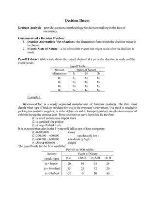
- 1. Decision Theory Decision Analysis – provides a rational methodology for decision making in the face of uncertainty. Components of a Decision Problem: 1. Decision Alternatives / Set of actions- the alternatives form which the decision maker is to choose. 2. Events/ State of Nature – a list of possible events that might occur after the decision is made. Payoff Tables- a table which shows the reward obtained if a particular decision is made and the event occurs. Payoff Table Decision States of Nature Alternatives S1 S2 S3 a1 r11 r12 r13 a2 r21 r22 r23 a3 r31 r32 r33 a4 r41 r42 r43 Example 1: Blockwood Inc. is a newly organized manufacturer of furniture products. The firm must decide what type of trick to purchase for use in the company’s operations. Use truck is needed to pick up raw material supplies, to make deliveries and to transport product samples to commercial exhibits during the coming year. Three alternatives were identified by the firm: (1) a small commercial import truck (2) a standard size pickup (3) a large flatbed truck It is expected that sales in the 1st year will fall in one of four categories: (1) 0-200,000 (low) (2) 200,000 – 400,000 (moderately low) (3) 400,000 – 600,000 (moderately high) (4) Above 600,000 (high) The payoff table for the firm would be: Payoffs in ‘000 profits Actions States of Nature (truck type) (1) L (2)ML (3) MH (4) H a1= Import 20 10 15 25 a2= Standard 15 25 12 20 a3= Flatbed -20 -5 30 40
- 2. Loss Tables – a table of opportunity cost corresponding to the losses incurred for not choosing the action corresponding to the highest payoff. Procedure: For each of the states of nature identify the highest payoff. Then subtract each entry in the column from the highest payoff. Loss Table Actions States of Nature (truck type) L ML MH H Import 0 15 15 15 Standard 5 0 18 20 Flatbed 40 30 0 0 Meaning of Losses: If we purchase Import and Even 1 occurred, we have no opportunity cost or regret since we have chosen the best out. If we had purchased standard, payoff is5 which is 5 less that the best, our opportunity cost would then be 5. Decision Trees- a graphical method of expressing in chronological order the alternative actions available to the decision maker and the possible states of nature. Types of nodes in a Decision Tree: 1. Decision Node – a point in time in which the decision maker selects and alternatives (represented by a rectangle). 2. Event Node- makes the occurrence of one of the possible states of nature after a decision is made. (represented by a circle) Represents an event that can occur at the Decision event node Node Branch (represents a course of Event action taken) Node
- 3. Decision Tree for Example 1: 0.2 20 ML 0.35 10 import 2 MH 0.3 15 H 0.15 25 L 0.2 15 ML 0.35 25 1 standard 3 MH 0.3 12 H 0.15 20 L 0.2 -20 ML 0.35 -5 flatbed 4 MH 0.3 30 H 0.15 40 Decision Making Under Uncertainty I. Non Probabilistic Decision Rules- management does not have reasonable estimates of the likelihood of the occurrence of various events. A. Maximin Rule For each decision alternative, identify the minimum payoff. Select the decision alternative having the largest of the minimum payoffs. Import 10 Therefore, Choose Standard 12 Standard Flatbed -20 Note: Maximin is a conservative or pessimistic decision rule. For each of the alternative we assume most event and we maximize their pessimistic outcome. B. Maximax Rule Identify the maximin payoff for each decision alternative. Select the decision alternative having the largest of the payoffs. Import 25 Therefore, Choose Standard 25 Flatbed Flatbed 40 Note: This is a risky or optimistic decision rule. We assume that for each decision alternative, the best event will occur. We maximize these optimistic outcomes.
- 4. C. Minimax Rule Here, we work with the loss table. For each decision alternative, identify the maximum possible loss. Select the decision alternative having the smallest of the losses. Import 15 Therefore, Choose Standard 20 Import Flatbed 40 Note: The rule is considered to be neither pessimistic nor optimistic. II. Probabilistic Decision Rule- the decision maker is able to assign probabilities to the various events that may occur. Sources of Probabilities: 1. Sample Information- a study or research analysis of the environment is used to assess the probability or occurrence of the event. 2. Historical Records- available from to files. 3. Subjective Probabilistic- probability may be subjectively assessed based on judgment, sample information and historical records. Example: Suppose that the firm in Example 1 has assessed the probabilities for the 4 sales levels as: P(1) = 0.20 P(3)= 0.30 P(2)= 0.35 P(4)= 0.15 What decision would be reached? Tool: Bayes Decision Rule – Select the decision alternative having the maximum expected payoff (minimum expected loss) Solution: 0.2 20 ML 0.35 10 import 2 MH 0.3 15 H 0.15 25 Therefore, purchase the standard truck. 18.35 18.35 L 0.2 15 ML 0.35 25 1 standard 3 MH 0.3 12 H 0.15 20 9.25 L 0.2 -20 ML 0.35 -5 flatbed 4 MH 0.3 30 H 0.15 40
- 5. Expected Value of Perfect Information – The worth to the decision maker to have access to an information source that would indicate for certain which of the events will occur. Consider previous example… If a perfect information source will reveal that eh following events will occur: Event Choice Payoff Probability 1 a1 20 0.2 2 a2 25 0.35 3 a3 30 0.3 4 a4 40 0.15 Expected Profit using Perfect Information Source (EPPI) would be: EPPI = 0.20(20) + 0.35(25) + 0.30(30) + 0.15(40) = 27.75 or P27,750 Without such perfect information, the expected profit based on Bayes Rule is P18.35 Therefore the expected value of perfect information would be: EVPI = 27.75 − 18.35 = 9.4 (or P 9,400) The primary use of EVPI is to determine the maximum amount a decision maker should be willing to pay for additional information (imperfect information) that could be employed to refine further the probability estimates. Sequential Decision Making- one in which the decision maker must initially select a decision alternative; once the outcome following that decision is observed, an opportunity again exists to select another decision alternative. Example: The city of Metropolis is planning to construct a street that will run through the city perpendicular to the main East-West Street. The city planner have to make a choice between a modern, wide (4-lane) street that would cost P2M or a lesser-quality, narrower street that would cost P1M. We shall denote these 2 alternatives as W1 and N1. After 4 years, depending on whether the traffic on the street turns out to be light or heavy( L1 or H1), the city will have the option of widening the street., The probability of these traffic condition are estimated by city planner and economists as P(L1)=0.25 And P(H1)=0.75. If W1 is selected, maintenance expenses during the 1st 4 years will be P5,000 or P75,000 depending whether the traffic is light or heavy. If N1 is selected, there costs are light or heavy. If N1 is selected, there costs are expected to be P 30,000 and P150, 000 respectively. Suppose street W1 is built, then at the end of 4 years, no further work is required. If heavy, either a minor or major repair must be made at costs of P150, 000 and P200, 000 respectively. If street N1 is built, then at the end of 4 years, if
- 6. traffic has been light, either a minor or major repair must be made at costs of P50,000 or P100,000 respectively. If traffic has been heavy, a major repair must be made at a cost of P900,000.traffic during the next 6 years will be classified as light or heavy (L2 or H2). The probabilities of these 2 events in years 1-4, are given as follows. P(L2/L1) = 0.75 P(L2/H1) = 0.10 P(H2/L1) = 0.25 P(H2/H1) = 0.90 Maintenance Costs over year 5-10 will depend on which street was built in year 1, what type of repair was made at the end of year 4, and the amount of traffic during years 5-10. Street Repair Traffic Maintenance Year 1 Year 5-10 Year 5-10 W1 None L2 200,000 H2 250,000 Minor L2 150,000 H2 175,000 Major L2 125,000 H2 100,000 N1 Minor L2 200,000 H2 250,000 Major L2 175,000 H2 150,000 a.) Construct a decision tree for this problem. b.) Determine the optimal sequential strategy for the city of Metropolis.
- 7. Solution: 0.2125 0.75 0.20 L2 .005 6 H2 0.3375 L1 75 0.25 0.25 0. 25 1 0. 2 2 0.10 0.125 0 0.1025 .7 5 L2 0.2 H1 7 5 7 .3 H2 7 0.3025 30 r 0. ajo 0. 0.10 25 0.90 0 75 M 4 0.10 0.15 M 32 2 0.1725 0. P2 1 in 5 M W L2 or 5 0.15 37 8 H2 2.3 0.90 0.175 1.975 1 Expected Value= Green Cost In M= Blue Probability = Red 1 .9 75 0.16875 0.75 0.175 L2 N1 1M 0.1 9 H2 0.15 26 r 0.25 0. ajo 5 87 0.2625 M 0.975 0.0 3 5 L1 5 .2 M 0. 25 92 0.2125 0.75 0.2 ino 2 5 3 0 .2 L2 6 r 0.05 10 H2 0.7 5 0.25 .25 1.2 H1 5 02 0.175 0 .1 0.1525 0.10 5 Major 0.90 L2 11 1.0525 H2 0.90 0.15 Year 1 – Build narrower street Year 4- Minor Repair if traffic is light Posterior Analysis – New information is obtained in order to refine the probability estimates of the events, thus, it is hoped, leading to a better decision. The information obtainable may be sample data, marketing research, data collected by electronic testing or surveillance or it may involve purchasing the advice of an expert. Prior Probabilities – Original probabilities of the various events. They exist prior to the use of sample information. Posterior Probabilities- revised probabilities calculated after the sample information is obtained.
- 8. Example: Suppose the fiorm in the truck eample acquires the services of a consulting firm, ABC Inc. ABC will conduct a market study that will result in one of the 2 outcomes: (1) O1 will be a favorable indicator of the market for the firm’s products. (2) O2 will be an unfavorable indicator O1 and O2 are referred to as sample outcome. The following conditional probabilities were arrived at from considerable ABC experience, using historical market-research record in ABC’s files and the statistician’s judgment P(Oj/Si) where:j=1 ,2 ; i=1,2,3,4 Sales S1 S2 S3 S4 O1 0.05 0.30 0.70 0.90 O2 0.95 0.70 0.30 0.10 Solution: Probability Tree P (K1∩K2) 0.01 O1 5 2 0.0 O 0. 9 2 5 0.19 S1 .2 0 0.105 O1 3 0.3 S2 O 0.35 0. 7 2 0 1 0.245 S3 0.3 0.21 0 O1 0 .7 4 O2 S4 5 0.3 0. 1 0 0.09 0.135 O1 0 0.7 5 O 0. 3 2 0 0.015 P(O1) = 0.01 + 0.105 + 0.21 + 0.135 = 0.46 P(O2) = 0.54
- 9. Revised Probabilities S 1 17 02 0. S2 3 0.228 Sample Computation: 2 S3 0.45 P ( S1 ∩ O1) P ( S1O1) = 65 0.2 S4 93 5 P (O1) 0.01 0. 1 O 46 = 0.46 =0.0217 1 O 0. 2 54 S 1 19 5 0. 3 S2 0.4537 3 S3 0.166 7 0. S4 02 78 Final Decision Tree: 16.902 L 0.0217 20 ML 0.2283 10 Import 4 MH 0.4565 15 H 0.2935 25 23.35 17.381 L 0.0217 15 ML 0.2283 25 Z1=favorable 5 2 standard 0.46 MH 0.4565 12 H 0.2935 20 23.35 L 0.0217 -20 ML 0.2283 -5 flatbed 6 MH 0.4565 30 H 0.2935 40 1 14.785 L 0.3519 20 ML 0.4537 10 import 7 MH 0.1667 15 H 0.0278 25 19.194 19.194 L 0.3519 15 ML Z2=unfavorable 0.4537 25 0.54 3 standard 8 MH 0.1667 12 H 0.0278 20 -3.114 L 0.3519 -20 ML 0.4537 -5 flatbed 9 MH 0.1667 30 H 0.0278 40 Summary of Decision Sample Outcome Action Profit O1 Flatbed(a3) P23,859.5
- 10. O2 Standard (a2) P19,177.40 Expected Value of Sample Information (Preposterior Analysis) - indicates whether it would pay us to purchase the sample information. EVSI= Expected Payoff with - Expected Payoff without Sample Information Sample Information For the truck Example: Expected Payoff with Sample Information = 0.46(23.8575) + 0.54(19.1774) = 21.330246 EVSI = 21.330246 − 18.35 = 2.980246 or (P2,980.25) Thus, we can hire the services of ABC ( for additional information) for as much as or less than P2,980.25. If ABC chooses P1000, the expected net gain of sampling would be: ENGS = 2,980.25 -1,000 = 1,980.25 Generally speaking, the sample information should be purchased if ENGS >0.