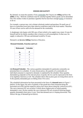
1. DEMAND AND ELASTICITY
By demand, we mean the quantity of any commodity that ‘buyers are willing and have the
ability to buy.’ Both the conditions must be satisfied together before goods can be demanded.
One who smokes wishes to purchase cigarettes but he must have enough money or resources
to do so.
For example, a person may visit a distant wholesale market and purchase 50 small cans of
beer at a somewhat lower price than what he would have paid in the local market. Therefore
50 cans of beer can be said to be his demand for the commodity.
A shopkeeper who begins with 200 cans of beer (which is his supply) may retain 10 cans for
himself and for his family members (this is known as self-consumption). In that case, his
supply is reduced to 190 cans and demand would be 10 cans.
Demand is an inverse (falling) function of the price.
Demand Schedule, Function and Law
D(demand) Schedule
qd P
10 0
8 1
4 2
1 3
0 4
(A) Demand Schedule : The various quantities demanded of a particular commodity are
presented here in a schedule. At some chosen prices, the quantity of a commodity an
individual consumer is expected to demand, is explained by the schedule. Since quantity
demanded (qd) depends on the relevant prices of goods, the two can be expressed in the form
of an algebraic function as well. The schedule shows that as price goes on rising (from zero to
4) the quantity demanded goes on falling (from 10 to zero).
The scheduled information has been presented in the form of a demand curve in Figure 1
(below). In the figure, the units of quantity of the goods have been measured along the
horizontal axis (OX) and the respective prices have been shown along the vertical axis (OY).
The curve intersects OY axis at point A which shows highest price at which quantity
demanded is zero. On the contrary the curve intersects OX axis at point B showing largest
quantity demanded where price is zero. Note that demand curve is sloping downward. This
follows the law of demand (given below).

2. Quantity Demanded qd
Figure 1
Law of demand: The law of demand explains the inverse relation between quantity and
price in general. It can be stated as follows:
Other things remaining equal), the quantity of a good demanded will rise (expand) with every
fall in its price and the quantity of a good demanded will fall (contract) with every rise in its
price."
This explains that qd, the quantity of a good demanded functionally depends on its price P.
However, the quantity demanded is also causally related to other factors such as income of an
individual (Y), prices of substitutes (Ps), number of members in the family (N) and the tastes
of the consumer (Z). In order to satisfy price-demand relation, the effect of these other
variables has been restrained by assuming them to be constant.
expansion and contraction in demand: On a given demand curve as we move downwards
from point A in the direction of B, the quantity demanded goes on rising with every
successive fall in price. This is known as expansion of demand. On the contrary, moving
from point B to A shows a fall in the quantity demanded with every successive rise in the
price. This is called as contraction in the demand. Therefore, in this case the price of the
quantity (and the change in it) plays an important part. Here, a change in the quantity
demanded is indicated with movement along the demand curve (up or down accordingly).
On the other hand, other factors are also likely to alter the quantity demanded. This can be
expressed by a shift in the curve. Such an upward shift in the demand curve (Figure 2) has
been shown by a new and higher demand curve (A1B1) in the figure.
Figure 2

3. At a given price OP on the original demand curve (AB), the quantity demanded is Oq but on
the new demand curve (A1B1) it has increased to Oq1. On the other hand, if we begin with the
A1B1 demand curve as the initial demand curve and consider demand to have reduced (to AB)
then the quantity demanded reduces from Oq1 to Oq. Such a change in the demand, arising
out of a shift in the demand curve is known as an increase (if it is towards the right of the
original demand curve) and a decrease (if it is towards the left of the original demand curve)
in the demand, respectively.
The demand curve may shift and quantity demanded may increase or decrease, due to
changes in a number of factors (apart from price), say the income (Y) of a consumer (when
he becomes richer or poorer). A similar effect can be noticed with a rise or fall in the price of
substitute (Ps) goods. For instance, tea and coffee or soaps of different brands are substitutes
of each other. Therefore a rise in price of pasta may result in a reduction in the consumption
of pasta and simultaneously an increase in the consumption of bread to that extent and vice
versa. Or the demand curve may shift and quantity demanded may increase at the old price
if there is a sudden increase in the number of members in a family (N), (say because of the
unexpected arrival of guests). Finally, a shift in the demand curve may also be the result of
the change in the tastes of a consumer. A cigarette or liquor consumer may become addicted
because of which his demand for such goods will rise remarkably even at the old price.
There is an important difference between the change in the quantity demanded of a
particular commodity and change in the demand for that commodity. While the former is
influenced by the single factor: price, the latter is influenced by various other factors apart
from price. A change in the quantity demanded is represented by a movement along the
demand curve, while a change in the demand is represented by a shift of the curve (towards
the left in case of a decrease and towards the right in case of an increase).
Exception to law of Demand
 It states that with a fall in price, demand also falls & with a rise in price demand also
rises.
Determinants of exception of law of demand
 Giffen’s paradox
 Veblen’s effect
 Fear of shortage
 Fear of future rise in price
 Speculation
 Conspicuous necessaries
 Emergencies
 Ignorance
 Necessaries
Elasticity of Demand
(A) Price Elasticity

4. i) Elasticity of Demand: Elasticity of demand can be classified into two major divisions: one
the highly elastic, unitary elastic and the highly inelastic type and two, the extreme cases of
the perfectly elastic and the perfectly inelastic type.
a) Highly elastic, Unitary elastic and highly inelastic: An actual rise or fall in the quantity
demanded with a small variation in the price may considerably differ for different goods
such as food, automobiles, film shows, garments, hardware materials, machines, land etc. In
other words it is important to know the extent of rise or fall in the demand with a given
change in the price for each individual good. This is exactly the purpose served by the
concept of price elasticity of demand.
Elasticity of demand is the degree of responsiveness with which quantity demanded changes
for a given change in price.
In other words it is a proportional change in the quantity demanded to a proportional
change in price.
Price Elasticity of demand is then the ratio of the proportional change in the quantity
demanded to the proportional change in price.
Proportional change in quantity can be expressed as where q1 is the initial and q2
is the new quantity demanded.
Proportional change in price is similarly where P1 is initial and P2 is the new price.
Elasticity ratio e is therefore,
Ed= q1-q2 * p1
Q1 p1-p2
Let’s illustrate this. In our demand schedule example above, when price changes from 2 to 3
units, the quantity demanded changes from 4 to 1 units. Substituting these values we have:
Note that the elasticity ratio 3/2 is more than one and has a negative sign. Both these are
important features. Numerical values explain the extent or degree of change in demand while

5. the sign of the ratio explains the direction of change. Since the law of demand is based on
the inverse relation between price and quantity, the elasticity of demand is always stated with
a negative sign.
The numerical value of elasticity can be equal to 1 (that is called ‘unit’) more than one or less
than one. In case of unit elastic demand (e = 1) both price and quantity (demanded) changes
occur in the same proportion.
If the value of elasticity exceeds one (e > 1) then the percentage or proportional change in
quantity demanded is greater than that in price and the good is said to be price elastic or
highly responsive to a change in price.
If the value of elasticity is less than one (e < 1) then the proportional change in quantity is
smaller than that in price and the demand for the good is said to be price inelastic or not very
responsive to a change in price.
There are four methods of measurement of elasticity of demand. These are percentage,
proportion, outlay and geometric or point elasticity methods.
Point Method:
Quantity demanded
Figure
In the figure, AB is the demand curve and at any point on this, the elasticity of demand can
be measured. At points R1, R and R2 the values of elasticity are:
At the mid point R on the demand curve, the value of elasticity is unit or equal to one. But
above point R such as at R1, the value of elasticity is more than one and demand is highly
elastic. On the other hand at a lower point such as R2 demand becomes inelastic as the value

6. of elasticity is less than one. In general as we move in the direction of the Y axis, demand
becomes more and more elastic. But as we move in the direction of the X axis, demand
becomes less and less elastic. In other words at every higher price demand is relatively more
elastic and at every lower price demand is relatively less elastic. This also explains that
elasticity of demand differs not only from commodity to commodity but also for the same
commodity at varying prices.
Total expenditure method
Elasticity of Demand Price Total Expenditure
Greater than unity Rise Down
Fall Up
Unity Rise Unchanged
Fall Unchanged
Less than unity Rise Up
Fall Down
Price of Quantity Total expenditure Effect on total Elasticity of
commodity expenditure demand
2 4 8 Same total expenditure Unity elastic
4 2 8
1 8 8
2 4 8 Less total exp. Greater than unity
4 1 4 More total exp.
1 10 10

7. 2 3 6 More total exp. Less than unity
4 2 8 Less total expenditure
1 4 4
• Proportionate method
change in quantity demanded
Initial demand
Change in Price
Initial price
b) Two extreme cases: Besides the three explained above, two more extreme values of price
elasticity of demand can be included in the analysis. These are:
(i) Perfectly Price Elastic: At this extreme, for any small decrease in price, the increase in
the quantity demanded is infinitely large. In such a case, demanders demand all they can.
Here the demand is said to be perfectly price elastic (e = that is infinity). This is represented
graphically as a horizontal demand curve (D1 in the figure above).
(ii) Perfectly Price Inelastic: At this extreme, for any change in price there is no change in
the quantity demanded. Therefore the demand is not responsive to any change in price. In this
case the demand is said to be perfectly price inelastic (e = 0). This is represented graphically
by a vertical demand curve (D2 in the figure above).
Determinants of price elasticity of demand:
 Nature of the demand
 Existence of substitutes
 Number of user of the commodity
 Durability & reparability of the commodity
 Possibility of postponing the use of a commodity.

8.  Level of income of the people
 Range of the price
 Habits
 Existence of complementary goods
Income elasticity: Demand is a function, besides price (P) also of the income (Y) of an
individual. However, income and demand hold a direct relationship, such that Y and Q rise or
fall together. Hence the sign of elasticity ratio in this case is normally positive. Let’s illustrate
this :
Assume that the values of Y and Q are as follows :
Y1 = 100 Q1 = 16
Y2 = 120 Q2 = 18
In this case the value of income elasticity ey will be:
(C) Cross Elasticity: Various goods A, B, C etc. hold a mutual relationship. As such if we
attempt to find the elasticity of demand for good B whenever the price of good A changes,
then it is called a cross elasticity ratio. However, the goods A and B may hold either of the
following relationships:
i) Substitutes : as in case of tea and coffee or different brands of toothpaste, television sets
etc. In this case, whenever the price of A rises the demand for A will fall but that of B will
rise. Therefore the relation between PA and QB is direct. Hence the sign of elasticity ratio will
be positive. This can be illustrated as:
PA QA QBS
10 8 8
12 6 10

9. ii) Complementary goods: Consider two complementary, good A - a vehicle and B -
gasoline. In this case, with a rise in the price of A the demand for A (QA) will fall and
similarly, the demand for B(QBC) will also fall. The sign of elasticity ratio will then be
negative in sign. This can be illustrated as follows:
PA QA QBC
5000 100 40
6000 80 35