• Ku, E.M., Elliott, S.J. and Lineton, B. (2009). ‘Nonlinear limit cycle oscillations in a state space model of the human cochlea,’ J. Acoust. Soc. Am., 126, (2), 739-750.

1. Limit cycle oscillations in a nonlinear state space model of the
human cochlea
Emery M. Ku,a Stephen J. Elliott, and Ben Lineton
Institute of Sound and Vibration Research, University of Southampton, Southampton, Hampshire SO17 1BJ,
United Kingdom
Received 14 March 2009; revised 20 May 2009; accepted 26 May 2009
It is somewhat surprising that linear analysis can account for so many features of the cochlea when
it is inherently nonlinear. For example, the commonly detected spacing between adjacent
spontaneous otoacoustic emissions SOAEs is often explained by a linear theory of “coherent
reflection” Zweig and Shera 1995 . J. Acoust. Soc. Am. 98, 2018–2047 . The nonlinear saturation
of the cochlear amplifier is, however, believed to be responsible for stabilizing the amplitude of a
SOAE. In this investigation, a state space model is used to first predict the linear instabilities that
arise, given distributions of cochlear inhomogeneities, and then subsequently to simulate the
time-varying spectra of the nonlinear models. By comparing nonlinear simulation results to linear
predictions, it is demonstrated that nonlinear effects can have a strong impact on the steady-state
response of an unstable cochlear model. Sharply tuned components that decay away exponentially
within 100 ms are shown to be due to linearly resonant modes of the model generated by the
cochlear inhomogeneities. Some oscillations at linearly unstable frequencies are suppressed over a
longer time scale, whereas those that persist are due to linear instabilities and their distortion
products. © 2009 Acoustical Society of America. DOI: 10.1121/1.3158861
PACS number s : 43.64.Kc, 43.64.Jb, 43.64.Bt, 43.40.Vn BLM Pages: 739–750
I. INTRODUCTION cochlea and are detectable in the ear canal Probst et al.,
1991 . OAEs provide a non-invasive indication of cochlear
Mammals rely upon an active mechanical process to en- health without the subject’s participation and are in wide
hance their sense of hearing. This takes place in the cochlea, clinical use Hall, 2000 . Clinicians generally class OAEs by
a fluid-filled organ responsible for amplifying and converting the stimulus used to evoke a response—such as clicks or
the acoustically induced motion of its structures into neural tones. In trying to analyze how OAEs arise, Shera and
impulses conveyed to the brain. A specialized structure in the Guinan 1999 proposed a classification paradigm based
human cochlea known as the organ of Corti OC performs upon the generation mechanisms of OAEs—such as linear
this complex task. Within the OC are approximately 12 000 reflection, nonlinear distortion, or some combination thereof.
hair-like cells called outer hair cells OHCs Pickles, 2003 . One class of OAE that, at first glance, seems to fit neatly into
These OHCs each contract and expand rapidly when a shear- both classification regimes is the spontaneous OAE SOAE .
ing motion opens and closes ion gates situated on the cells’ SOAEs are narrowband tones that propagate out of the
stereocilia, thus inducing first mechano-electrical and then cochlea without a stimulus and are detectable in the ear canal
electro-mechanical transduction Ashmore, 1987 . The col- with a sensitive microphone Probst et al., 1986 . Most hu-
lective efforts of the OHCs comprise a system termed the man SOAEs are detected between 0.5 and 6 kHz, with the
cochlear amplifier CA . majority falling in the range of 1–2 kHz. Both the frequen-
Experimental studies of the CA in animals have shown cies and amplitudes of SOAEs are remarkably stable over
that it is capable of amplifying the magnitude of basilar time Probst et al., 1991 . These emissions are indicative of a
membrane BM motion by up to 45 dB at low excitation healthy cochlea, being present in approximately 70% of all
levels Robles and Ruggero, 2001 . At moderate levels, the
normal-hearing individuals Talmadge and Tubis, 1993; Pen-
CA begins to saturate and exhibit distortion effects; recent
ner and Zhang, 1997 . It is also well-known that the spectra
experimental work suggests that the distortion generated by
of evoked emissions differ somewhat from those of SOAEs
the CA in mice may be due to the tip-links connecting adja-
e.g., Wable and Collet, 1994 . So-called “long-lasting”
cent stereocilia Verpy et al., 2008 . At high levels, the out-
evoked responses, also referred to as synchronized spontane-
put of the active CA is negligible relative to the passive
ous otoacoustic emissions SSOAEs , are sometimes re-
excitation of the BM. The nonlinearity of the CA is thus an
corded by extending the click evoked OAE CEOAE acqui-
intrinsic feature of the normal cochlea that contributes to its
enormous dynamic range, which is on the order of 120 dB sition window from 20 to 80 ms Gobsch and Tietze, 1993;
sound pressure level SPL in humans Gelfand, 1998 . Sisto et al., 2001; Jedrzejczak et al., 2008 . The origin of this
One important group of cochlear epiphenomena is otoa- long-lasting ringing continues to be debated.
coustic emissions OAEs , sounds that propagate out of the Early theoretical work by Gold 1948 that pre-dated the
discovery of OAEs predicted the existence of SOAEs due to
instability in locally active elements. However, after the dis-
a
Author to whom correspondence should be addressed. Electronic mail: covery of OAEs by Kemp 1979 , there were numerous re-
emk@soton.ac.uk ports of a commonly detected spacing between adjacent
J. Acoust. Soc. Am. 126 2 , August 2009 0001-4966/2009/126 2 /739/12/$25.00 © 2009 Acoustical Society of America 739

2. SOAE frequencies Dallmayr, 1985, 1986; Talmadge and order to better match the predicted variation of TW wave-
Tubis, 1993; Braun, 1997 . Such regularity seemed to be at length with position in the human cochlea, minor revisions to
odds with a local oscillator framework, where one might the model parameter values are presented. The implementa-
assume unstable elements to be randomly distributed. tion of a saturation nonlinearity in the model’s CA is then
An alternative explanation of SOAE generation assumes described.
multiple traveling wave TW reflections between a cochlear Section III presents the results from a variety of simula-
reflection site and the middle ear boundary at its base, analo- tions. A set of linear stability tests is first presented. The
gous to standing waves in homogenous media Kemp, 1979; results of a nonlinear time domain simulation involving a
Zwicker and Peisl, 1990; Zweig, 1991; Shera and Zweig, single linear instability, generated by introducing a step-
1993; Talmadge and Tubis, 1993; Zweig and Shera, 1995; change in feedback gain as a function of position, are then
Allen et al., 1995; Talmadge et al., 1998; Shera and Guinan, analyzed in detail and interpreted in terms of TWs. This is
1999; Shera, 2003 . Shera and Zweig 1993 and Zweig and expanded upon by running a nonlinear simulation of a model
Shera 1995 developed a linear “coherent reflection” hy- with a small range of linear instabilities, generated by a spa-
pothesis that built upon the cochlear standing wave theory tially restricted region of inhomogeneities in the feedback
and also accounted for the cause of the spacings between gain. Finally, simulations of nonlinear cochleae with a large
SOAEs. number of linear instabilities across the cochlea’s frequency
Previous SOAE modeling work followed various av- range are performed; these instabilities are generated by in-
enues of research. Early reports showed that SOAEs can be troducing inhomogeneities in the feedback gain all along the
suppressed and otherwise affected by external tones e.g., cochlea, as have been postulated to exist in the biological
Zwicker and Schloth, 1984 . Phenomenological models us- cochlea.
ing van der Pol oscillators were applied to describe the be-
havior of isolated SOAEs e.g., Bialek and Wit, 1984; Wit,
1986; van Dijk and Wit, 1990; van Hengel and Maat, 1993; II. MODEL DESCRIPTION
Murphy et al., 1995 . However, the success of the coherent-
reflection theory in predicting many features of OAEs The basis of the model used in this investigation is that
prompted modelers to try to replicate these findings in com- of Neely and Kim 1986 . Elliott et al. 2007 showed that it
plete mechanical models of the cochlea. Including random is possible to recast this frequency-domain system in state
perturbations in the smoothly varying mechanical parameters space. State space is a mathematical representation of a
was found to generate reflections and cochlear standing physical system that is commonly used in control engineer-
waves in a variety of models e.g., Talmadge et al., 1998; ing Franklin et al., 2005 . One advantage of this formulation
Talmadge et al., 2000; Shera et al., 2005; Elliott et al., 2007 . is that there are widely available, well-developed tools to
The nonlinear time domain simulations of Talmadge study the behavior of such models. For example, it is
et al. 1998 showed amplitude-stabilized limit cycle oscilla- straightforward to simulate state space models in the time
tions LCOs similar to SOAEs, but the number, frequencies, domain using the ordinary differential equation solvers in
and amplitudes were not predicted. In contrast, the linear MATLAB.
stability tests performed by Ku et al. 2008 predicted the This section presents some minor revisions to the linear
number and frequencies of instabilities but did not account state space model and the necessary additions in order to
for any nonlinear effects that might affect the resultant account for CA nonlinearity in the time domain. Interested
LCOs. The nonlinear phenomena that pertain to cochlear readers are directed to previous work for a more in-depth
LCOs may include mutual suppression, the generation of description of the model Neely and Kim, 1986; Ku et al.,
harmonic and intermodulation distortion, and mode-locking 2008; Ku, 2008 and the state space formulation Franklin
as in musical wind instruments Fletcher, 1999 . et al., 2005; Elliott et al., 2007 .
A. Aims and overview A. The linear model
This paper is concerned with the impact of cochlear non- The active linear model seeks to represent a human co-
linearity upon the linear state space model’s predictions of chlea’s response to low-level stimuli where the CA is work-
SOAEs. This work is an extension of the cochlear modeling ing at full strength. The Neely and Kim 1986 microme-
findings presented in two previous papers. In the first, Elliott chanical model is based upon physical structures of the OC;
et al. 2007 introduced a state space framework for a clas- it consists of a two-degree-of-freedom system with an active
sical model of the cochlea Neely and Kim, 1986 . In the element in a feedback loop. This active element provides
second, Ku et al. 2008 applied the state space model to “negative damping” such that the cochlear TW due to a pure
demonstrate how predictions of the coherent-reflection tone is enhanced basal of its peak. The original model de-
theory of SOAE generation Shera and Zweig, 1993; Zweig scribed the cat cochlea; Ku et al. 2008 revised the param-
and Shera, 1995 can be observed in a linear, non-scaling- eters to account for the characteristics of a human cochlea.
symmetric model of the cochlea. The present paper investi- Minor modifications are provided here to reproduce the
gates how linear instabilities interact and evolve in a nonlin- variation in TW wavelength as a function of position, as
ear model of the cochlea to form LCOs similar to SOAEs. deduced from OAE data Shera and Guinan, 2003 . The pa-
A short review of the linear model is given in Sec. II. In rameters that have been updated from Ku et al. 2008 are
740 J. Acoust. Soc. Am., Vol. 126, No. 2, August 2009 Ku et al.: Cochlear limit cycle oscillations

3. TABLE I. Model parameters for the revised quantities to represent a human B. The nonlinear model
cochlea.
Including nonlinearity in a cochlear model can add com-
Quantity Revised formula SI Units plexity and greatly increase the computational intensity of a
1.65 109e−279 x+0.00373 N m−3
given simulation. However, there are many fundamental at-
k1 x
c1 x 9 + 9990e−153 x+0.00373 N s m−3 tributes of the cochlea that are not captured in a linear model.
m1 x 4.5 10−3 kg m−2 The primary source of saturating nonlinearity in the cochlea
k2 x 1.05 107e−307 x+0.00373 N m−3 is the relative decrease in the OHC feedback force with in-
c2 x 30e−171 x+0.00373 N s m−3 creasing driving level; this effect is sometimes referred to as
m2 x 7.20 10−4 + 2.87 10−2x kg m−2 “self-suppression” in the literature Kanis and de Boer,
k3 x 1.5 107e−279 x+0.00373 N m−3 1993 .
c3 x 6.6e−59.3 x+0.00373 N s m−3 To incorporate a saturation nonlinearity into the state
k4 x 9.23 108e−279 x+0.00373 N m−3 space model, the feedback gain, , is made to depend on the
c4 x 3300e−144 x+0.00373 N s m−3
instantaneous shear displacement between the BM and the
TM, c. This can be expressed in state space as a time-
varying version of the system matrix in Eq. 2 , A t , so that
shown in Table I. The micromechanical model and physical
meaning of these quantities are described in Elliott et al. ˙
x t = A t x t + Bu t , 4
2007 . where
The TW wavelength at its peak is approximately 0.5 mm
at locations basal of 5 mm in the model; apical of this posi- A t = Apassive + c t Aactive . 5
tion, the TW wavelength increases linearly with position ap- The current model does not make any assumptions re-
proaching 1.5 mm at the apex. The other TW characteristics garding the precise mechanisms of the electro-mechanical
such as enhancement and tonotopic tuning are broadly un- transduction in OHCs. The goal was to integrate the least
changed. A thorough review of the model and its responses complex saturation function into the model that also pro-
to stimuli can be found in Ku 2008 . duces realistic results. A first order Boltzmann function is
The macromechanical formulation of the state space used to approximate the local saturation of the CA feedback
model Elliott et al., 2007 is based upon the work of Neely force with level because its shape well approximates the
1981 and Neely and Kim 1986 . A finite difference ap- input-output pressure to intracellular voltage characteristics
proximation is used to discretize the spatial derivatives in the of OHCs measured in isolation e.g., Cody and Russell,
wave equation and boundary conditions of the model. The 1987; Kros et al., 1992 . This function is applied to the dis-
local activity of the cochlear partition segments is related to placement input of the feedback loop that determines the
the fluid mechanics by the one-dimensional wave equation in OHC force in the time domain:
matrix form:
1 1
¨
Fp t − w t = q, 1 f u = − , 6
1 + e−u/ 1+
¨
where p t and w t are the vectors of pressure differences
where u is the input displacement, sets the saturation point,
and cochlear partition accelerations, F is the fluid-coupling
affects the slope of the output, and affects the asymme-
matrix, and q t is the vector of source terms that serves as
try of the function. In order to set the slope of the function to
the input to the macromechanical model; in the baseline form
unity for small input displacements, u, it is necessary to con-
of the model, q t is zero except at the stapes. The cochlear
strain
micromechanics of isolated partition segments are described
by individual matrices. When Eq. 1 is substituted into an
= 2. 7
equation combining all the uncoupled elemental matrices, 1+
including the middle ear boundary at the base and the heli-
cotrema at the apex, the dynamics of the fluid-coupled model The free parameter, , is set to 3. The function and its slope
can be described by the state space equations are illustrated in Fig. 1.
In order to determine t , the shear displacement wave-
˙
x t = Ax t + Bu t 2 form is passed through the Boltzmann function and scaled by
and the waveform itself:
y t = Cx t + Du t , 3 f c t
c t = . 8
c t
where A is the system matrix that describes the coupled me-
chanics, x t is the vector of state variables which include The nonlinearity is thus both instantaneous and memory-less.
BM and tectorial membrane TM velocities and displace- While the saturation point variable of the Boltzmann
ments, B is the input matrix, u t is a vector of inputs equal function, , is set to 1 in Fig. 1 for illustration purposes, it is
to F−1q t , y t is the output variable BM velocity in this varied as a function of position in this model of the nonlinear
case , C is the output matrix, and D is an empty feed-through cochlea. Due to the decrease in BM stiffness with distance
matrix. The details of this formulation are described by El- from the stapes, the cochlear partition will deflect more at the
liott et al. 2007 . apex relative to the base when driven by a constant pressure.
J. Acoust. Soc. Am., Vol. 126, No. 2, August 2009 Ku et al.: Cochlear limit cycle oscillations 741

4. 1
a)
0.5
Output
0
−0.5
−1
−1.5 −1 −0.5 0 0.5 1 1.5
Input
1.5
b)
Slope of Output
1
0.5
0
−1.5 −1 −0.5 0 0.5 1 1.5
Input
FIG. 1. Boltzmann function characteristics with saturation parameter = 1.
a Output vs input. b Slope of output vs input.
FIG. 3. Variation in the spacings between adjacent linear instabilities plotted
against the geometric mean frequency of adjacent instabilities. The low-
Thus, x has a considerable impact upon the results of the wavelength cut-off frequency of the random variations in x is set to 0.19
simulation. In order to generate a sensible x , the maxi- mm. The darkened dots represent values of the spacings that fall within the
1 standard deviation of the mode within 15 log-spaced bands see Fig. 3 of
mum displacement at a given location, calculated across fre- Shera 2003 . A trend line is fitted to the modes of each band.
quencies in the coupled linear model, is used as a template
for x at locations approximately 6 mm x 27 mm; is
otherwise smooth distribution of x . The statistics of these
fixed to constant values outside this range. This distribution
instabilities satisfied a variety of predictions of the coherent
is normalized to the maximum value and scaled by 10 nm; a
reflection theory of SOAE generation. One aspect of human
saturation point that is approximately 1 nm at the base yields
SOAE data that was not accounted for in the model of Ku et
results that are similar to various experimental measurements
al. 2008 is the variation in SOAE spacings with frequency
made in animals Robles and Ruggero, 2001 . The final dis-
Shera, 2003 . This is addressed by the revised set of param-
tribution of x is shown in Fig. 2.
eters presented in Table I.
Figure 3 represents the summarized stability tests of 200
III. Results cochlear models. Random “dense” distributions of x were
A. Linear stability tests generated by filtering Gaussian white noise with fifth order
Butterworth filters using a wide bandwidth of spatial fre-
One of the advantages of the state space formulation is quencies see Ku et al., 2008; Lineton, 2001 . In contrast to
that it is possible to test the linear stability of a model. This a “sparse” distribution of x , a dense distribution contains
is accomplished by calculating the eigenvalues of the system significant spatial wavenumber content at one-half the TW
matrix, A, which correspond to the system poles Franklin wavelength at its peak at all locations in the cochlea Ku,
et al., 2005 . Ku et al. 2008 generated linear instabilities in 2008 . The peak-to-peak variation in x was held at a con-
the state space model by introducing inhomogeneities in the stant of 15%. The results of Fig. 3 show good qualitative
agreement with statistics of measured SOAE spacings in hu-
10 mans see Fig. 3 of Shera, 2003 .
9
B. Nonlinear simulation: Step-change in „x…
8
In order to better understand the LCOs that develop in
7
unstable nonlinear cochleae, the response of a model with a
δ(x) [nm]
6 single linear instability is analyzed in detail. This instability
5
is generated in the state space cochlea at 1.214 kHz by ap-
plying a step-distribution of feedback gain with x
4
18.9 mm = 1 and x 18.9 mm = 0.85. As shown in
3 Fig. 4, a single pole exhibits a positive real part,
2
= 0.031 ms−1, thus indicating that the system is unstable. It is
also possible to create a model with a single unstable pole by
1
applying a random x , though a step-distribution of x
0 has the added benefit that there is no ambiguity in the loca-
0 5 10 15 20 25 30 35
Position along the cochlea [mm] tion of the reflection site.
FIG. 2. Nonlinear saturation point of the micromechanical feedback loops The stability plot has been introduced previously as a
as a function of position, x . convenient way of representing the poles of the system El-
742 J. Acoust. Soc. Am., Vol. 126, No. 2, August 2009 Ku et al.: Cochlear limit cycle oscillations

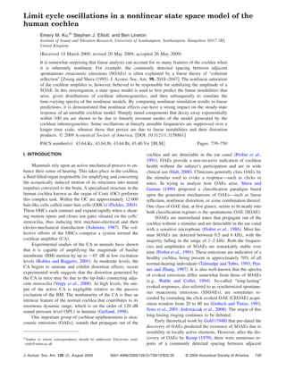
5. 0.5
CF at x = 18.9 mm
ωi = 1.214 kHz, σi = 0.031 ms−1
0
−0.5
σ [ms−1]
−1
1
γ
0.9
−1.5
0.8
0 10 20 30
Position along the cochlea [mm]
−2
0 0.5 1 1.5 2 2.5 3
Frequency [kHz]
FIG. 4. Stability plot of a cochlear model with a step-change in x , shown FIG. 5. Click response of the unstable nonlinear cochlear model described
in the inset. A vertical line marks characteristic frequency of a baseline in Fig. 4. BM velocity is plotted against time and position along the cochlea.
cochlea at the location of the step-change in x . The unstable pole is
circled and described by annotations.
frames are examined, only the response at the linearly un-
liott et al., 2007; Ku et al., 2008 . The imaginary part of a stable frequency and its harmonics persist. The frequency of
pole, plotted on the horizontal axis in kilohertz, represents its the primary LCO in Fig. 6 d is within 0.04% of the linear
frequency; the real part of a pole, plotted on the vertical axis prediction, 1.214 kHz. The spectral resolution of the panels
in inverse milliseconds ms−1 , represents its rate of expo- improves as longer time windows are analyzed in later time
nential growth or decay. Thus, a pole with a positive real part frames.
indicates that the system is unstable. Note that Fig. 4 only
shows a small portion of the overall stability plot in order to
emphasize the instability.
When the unstable model presented in Fig. 4 is excited 1. Interpretation in terms of TWs
in the nonlinear time domain by a click at the stapes, mul-
The discrete Fourier transform DFT of the BM veloc-
tiple TW reflections occur between the step-discontinuity in
ity is computed from 1000 t 3000 ms at the frequency of
x and the middle ear boundary condition to form a co-
the LCO, 1.214 kHz, for each location in the cochlea; the
chlear standing wave. This becomes a LCO over time due to
magnitude and phase are shown in Fig. 7. In the steady-state
the saturation of the CA. The cochlear response is plotted as
response of the model with a single linear instability due to a
a function of position and time in Fig. 5. Backward TWs are
step-change in x , the peak in the TW phase as a function
visible after the initial transient wavelet passes through the
of position occurs basal to the peak in magnitude. This is
location of the discontinuity, x = 18.9 mm. The spectrum of
the pressure at the stapes also varies with time; this is of
particular interest because it is understood that this pressure 10 ≤ t ≤ 110 ms 50 ≤ t ≤ 550 ms
20 0.3 20 0.3
induces motion in the middle ear bones to generate OAEs in a) b)
Pressure [dB SPL]
Pressure [dB SPL]
0 0.2 0 0.2
the ear canal. It is also possible to calculate the resulting −20 −20
σ [ms−1]
σ [ms−1]
0.1 0.1
pressure in the ear canal, though this is left to future work in −40
0
−40
0
order to simplify the interpretation of results. −60
−0.1
−60
−0.1
−80 −80
The pressure spectrum at the base is plotted over four −100 −0.2 −100 −0.2
time windows in Figs. 6 a –6 d . Superimposed on each −120
0.6 0.9 1.3 1.9 2.8 4.1 6
−0.3 −120
0.6 0.9 1.3 1.9 2.8 4.1 6
−0.3
frame is the stability plot over this frequency range. Blunt Frequency [kHz] Frequency [kHz]
500 ≤ t ≤ 1000 ms 1000 ≤ t ≤ 3000 ms
peaks are visible in the pressure spectrum of Fig. 6 a at 20 0.3 20 0.3
c) d)
Pressure [dB SPL]
Pressure [dB SPL]
frequencies corresponding to the near-unstable poles as well 0 0.2 0 0.2
−20 −20
as the single unstable frequency. The levels of these peaks
σ [ms−1]
σ [ms−1]
0.1 0.1
−40 −40
also seem well-correlated with the relative magnitudes of the −60
0
−60
0
real parts of the poles, i. This is consistent with the calcu- −80
−0.1
−80
−0.1
−0.2 −0.2
lated linear transient response of a system with damped −100 −100
−120 −0.3 −120 −0.3
modes, which would include spectral components at each of 0.6 0.9 1.3 1.9
Frequency [kHz]
2.8 4.1 6 0.6 0.9 1.3 1.9
Frequency [kHz]
2.8 4.1 6
the resonant frequencies of the system. The decay of these
components is determined by the magnitude of the real parts FIG. 6. Superimposed stability plots of the linear system right axes and the
spectrum of the pressure at the base of a nonlinear, unstable cochlea left
of the corresponding poles, i.
axes given four time windows: a 10 t 110 ms; b 50 t 550 ms;
In this nonlinear system, distortion is visible at the sec- c 500 ms t 1500 ms; d 1000 t 3000 ms. The unstable pole is
ond and third harmonics of the fundamentals. As later time plotted with a dark x; stable poles are plotted with light x’s.
J. Acoust. Soc. Am., Vol. 126, No. 2, August 2009 Ku et al.: Cochlear limit cycle oscillations 743

6. −130
a) Max amplitude basal and 1 mm apical of the / x = 0 place. The imposed
|ξ˙b | [dB re: 1 m/s]
−140
step-discontinuity in x coincides with both the apical end
−150
point of the negative damping region, shown in Fig. 7 as a
−160
shaded area, and the location of maximum TW magnitude.
−170
f0 = 1.214 kHz When the initial forward traveling wavelet passes
−180
−190
Negative damping region ∂φ/∂x = 0 through the negative damping region, it is amplified at the
8 10 12 14 16
Position along the cochlea [mm]
18 20 22 frequency of the instability. This response peaks at the loca-
tion of the step-discontinuity, which causes a wavelet to be
5
b) reflected back toward the base. As this reflected wavelet
Forward TW
4 passes back through the negative damping region, it is again
ξ˙b [cycles]
3 amplified. The amplification of backward TWs in a one-
2 Standing Wave dimensional model has been previously demonstrated by Tal-
1
madge et al. 1998 . The peak in the phase response repre-
Backward TW
sents the only position along the BM where the amplitudes
0
8 10 12 14 16
Position along the cochlea [mm]
18 20 22 of forward and backward TWs are equal; as a result, the TW
is “standing” at the / x = 0 location. The nearby ripples in
the magnitude are likely due to constructive and destructive
FIG. 7. Steady-state a magnitude and b phase of the BM velocity re-
sponse as a function of position at the unstable frequency. A solid vertical interference of forward and backward TWs; this is only vis-
line marks the location of the peak in magnitude at x = 18.9 mm, and a ible where these TW components are approximately equal in
dashed vertical line marks the location of the peak in the phase. The region amplitude.
of negative damping, determined by evaluating the real part of the BM
Perhaps contrary to one’s intuition, the roundtrip TW
impedance at a frequency of 1.214 kHz in a baseline active cochlea, is
shaded. delay is still twice the forward delay. However, this is no
longer apparent from the phase plot as the backward TWs are
sometimes interpreted to mean that the TW is reflected basal hidden “under” the dominant forward TWs in the overlap
to the location of the impedance discontinuity, resulting in a region basal to the characteristic place. Similar plots are gen-
roundtrip delay that is less than twice the forward delay. The erated when forward TWs are reflected by spatially random
actual physical meaning of the data can be clarified by ex- inhomogeneities in linear wave models Neely and Allen,
amining this result in closer detail. 2009 .
The dominant direction of wave propagation in this co-
chlear model is indicated by the sign of the slope of the 2. Linear analysis of the steady-state nonlinear
phase response as a function of position, / x. For in- response
stance, a positive phase slope indicates a predominantly Given both steady-state pressure and velocity, it is pos-
backward TW, a zero phase slope indicates a standing wave, sible to reconstruct the effective linear feedback gain as a
and a negative phase slope indicates a predominantly for- function of position in this nonlinear simulation, eff x ; this
ward TW. It is not a coincidence that the position where the line of reasoning follows from de Boer’s 1997 EQ-NL
phase slope is zero is located within the negative damping theorem. Solving the BM impedance equation Eq. 12 in
region at this frequency, which extends approximately 2 mm Neely and Kim, 1986 for the effective feedback gain yields
Z 1Z 2 + Z 1Z 3 + Z 2Z 3 − Z 1 + Z 2 P x / ˙ b x
eff x f=1.214 kHz = , 9
Z 2Z 4 f=1.214 kHz
where P x is the pressure difference across the cochlear space cochlea to study its stability, as shown in Fig. 9. eff is
partition, ˙ b x is the BM velocity, and Zi are the frequency- set= 0.85 for x 23 mm in this linear stability test. The pole
and position-dependent impedances of the micromechanical located at 1.214 kHz is no longer unstable, but its real part is
model Neely and Kim, 1986 . The distribution of eff x that very nearly zero. The effective linear system will ring at
is calculated from the above nonlinear simulation at steady- 1.214 kHz with a velocity distribution that is almost identical
to that of Fig. 7, but its oscillations will neither grow nor
state is presented in Fig. 8, in addition to the original im-
decay significantly with time; this is consistent with the ob-
posed x . In the region just basal to the TW peak, where
served LCO behavior in the nonlinear simulation. From this,
negative damping takes place, eff x is less than the imposed it is possible to deduce that the amount of work done by the
gain. The effective gain calculation breaks down beyond x CA at this frequency is equal to the losses in the cochlear
23 mm, where the TW becomes evanescent. model, as predicted by the coherent-reflection theory Shera,
It is informative to now apply eff x to a linear state 2003 .
744 J. Acoust. Soc. Am., Vol. 126, No. 2, August 2009 Ku et al.: Cochlear limit cycle oscillations

7. 1.05 0.5
1 0
Feedback gain γ
−0.5
σ [ms−1]
0.95
0.9 −1
1.1
γ(x)
1
−1.5
0.85
0.9
0 10 20 30
Imposed γ(x) Position along the cochlea [mm]
Effective Linear γ(0 ≤ x ≤ 23 mm) −2
0.8 0 0.5 1 1.5 2 2.5
0 5 10 15 20 25 30 35
Position along the cochlea [mm] Frequency [kHz]
FIG. 8. The effective linear feedback gain of the nonlinear simulation at FIG. 10. Stability of a linear cochlear model given a windowed-perturbed
steady-state as a function of position — and the original imposed feedback gain distribution, shown in the inset. Five unstable poles result.
gain – – .
ones at its midpoint; zeros are padded outside this range, and
C. Nonlinear simulations: Random changes in „x… the function is centered at x = 19 mm. By applying this ex-
When multiple linear instabilities are predicted, it is pos- tended Hann window to a dense distribution of random in-
sible that nonlinear interactions between the resultant LCOs homogeneities in x , five linear instabilities are generated
will suppress one another or generate intermodulation distor- at f = 0.979, 1.080, 1.145, 1.229, 1.296 kHz, as shown in
tion. This subsection presents simulations of cochleae with Fig. 10. As before, the nonlinear pressure spectrum at the
dense inhomogeneities that express a broad band of spatial base of the cochlear model is calculated across four time
frequencies, as in Ku et al. 2008 . In the first instance, a windows and compared with the linear stability plot in Fig.
linearly unstable system with a spatially limited region of 11.
inhomogeneity is generated to study the interactions of a The evolution of the nonlinear response shown in Fig.
small number of instabilities. Subsequently, systems with in- 11 is analogous to that of Fig. 6. In the earliest time frame
homogeneities distributed along the lengths of the cochlear Fig. 11 a , there are peaks in the pressure spectrum at all of
models are examined. In each case, the spectral content of the resonant modes generated by the inhomogeneities—both
LCOs in nonlinear time domain simulations is compared stable and unstable. However, as time progresses, the peaks
against the frequencies of the linear instabilities. at the near-unstable frequencies die away. In contrast to the
case of the isolated instability, not all of the linearly unstable
1. Isolated region of inhomogeneity frequencies are represented at steady-state, as seen in Fig.
11 d . Peaks are also detected at frequencies that correspond
In order to restrict the inhomogeneous region in space, a
3.5 mm long Hann window is extended by inserting 3.5 mm
10 ≤ t ≤ 110 ms 50 ≤ t ≤ 550 ms
20 0.3 20 0.3
a) b)
Pressure [dB SPL]
Pressure [dB SPL]
0 0
0.5 0.2 0.2
−20 −20
σ [ms−1]
σ [ms−1]
0.1 0.1
−40 −40
0 0
ωi = 1.214 kHz, σi = −0.000035 ms−1 −60 −60
−0.1 −0.1
0 −80 −80
−100 −0.2 −100 −0.2
−120 −0.3 −120 −0.3
0.6 0.7 0.85 1 1.25 1.5 1.8 0.6 0.7 0.85 1 1.25 1.5 1.8
Frequency [kHz] Frequency [kHz]
−0.5
σ [ms−1]
500 ≤ t ≤ 1500 ms 1500 ≤ t ≤ 3000 ms
20 0.3 20 0.3
c) d)
Pressure [dB SPL]
Pressure [dB SPL]
f1 f3
0 0.2 0 0.2
−20 −20 f2
−1
σ [ms−1]
σ [ms−1]
0.1 0.1
−40 −40
0 0
−60 −60
1 −0.1 −0.1
−80 −80
γ
0.9
−1.5 −100 −0.2 −100 −0.2
0.8
0 10 20 30 −120
0.6 0.7 0.85 1 1.25 1.5
−0.3
1.8
−120
0.6 0.7 0.85 1 1.25 1.5
−0.3
1.8
Position along the cochlea [mm] Frequency [kHz] Frequency [kHz]
−2
0 0.5 1 1.5 2 2.5 3 FIG. 11. Simultaneous plots of the linear system stability right axes and
Frequency [kHz] the spectrum of the pressure at the base of the nonlinear cochlear model left
axes given four time windows: a 10 t 110 ms; b 50 t 550 ms;
FIG. 9. Linear stability plot as determined by applying the effective linear c 500 t 1500 ms; d 1500 t 3000 ms. Unstable poles are plot with
gain as a function of position shown in Fig. 8. Note that the applied gain has dark x’s; stable poles are plot with light x’s. Three linearly unstable frequen-
been set to 0.85 for x 23 mm. cies, f 1, f 2, and f 3, are indicated.
J. Acoust. Soc. Am., Vol. 126, No. 2, August 2009 Ku et al.: Cochlear limit cycle oscillations 745

8. Near−Unstable frequencies 1000 ≤ t ≤ 3000 ms
Pressure [dB SPL]
a) f = 0.8 kHz
a) Selected LCOs
0 0
LCOs at ±1% of linear instability
Magnitude of Pressure Component [dB SPL] f = 0.848 kHz
f = 0.923 kHz Linearly unstable frequencies
f = 1.033 kHz
−50 −50
f = 1.359 kHz
f = 1.597 kHz
−100
−100
0 500 1000 1500 2000 2500 3000
0 0.5 1 1.5 2 2.5
Frequency [kHz]
Linearly unstable frequencies
500
b) ∆f = 83 Hz b)
0
∆f = 2*83 Hz
∆f = 3*83 Hz
∆f [Hz]
−50 f1 = 0.979 kHz f = 1.08 kHz f2 = 1.145 kHz 249
f3 = 1.229 kHz f = 1.296 kHz 166
−100 83
0 500 1000 1500 2000 2500 3000 0
0 0.5 1 1.5 2 2.5
Geometric mean frequency [kHz]
Distortion product frequencies
20
c) 2f1−f2 = 0.813 kHz 2f2−f1 = 1.311 kHz 2f2−f3 = 1.061 kHz
0 FIG. 13. The steady-state basal pressure spectrum is displayed across a
−20 2f3−f2 = 1.313 kHz 2f1−f3 = 0.729 kHz 2f3−f1 = 1.479 kHz limited frequency range in panel a . A star marks selected LCOs. Se-
−40
lected LCOs that also correspond to linearly unstable frequencies and spac-
−60
ings are denoted by a circle . The horizontal axis of panel b represents
−80 f1 = 0.979 kHz
f2 = 1.145 kHz the geometric mean of the two adjacent limit cycle frequencies; the vertical
−100
f3 = 1.229 kHz axis represents the separation between LCOs in Hz. Dotted, dot-dashed, and
−120
0 500 1000 1500 2000 2500 3000 dashed horizontal lines are drawn at f = 83, 2 83, 3 83 Hz, respec-
Time [ms] tively.
FIG. 12. Variation in the magnitude of basal pressure frequency components
in an unstable cochlea as a function of time. Near-unstable and linearly
unstable frequencies are shown in a and b , respectively, while distortion linearly unstable frequencies that persist in amplitude: f 1
product frequencies are shown in panel c . Every curve consists of 15 data = 0.979 kHz, f 2 = 1.145 kHz, and f 3 = 1.229 kHz. The mag-
points, where each value represents the DFT of 200 ms of data with no
overlap between adjacent windows. nitudes of the distortion products at 2f 1 − f 3 and 2f 3 − f 1 mir-
ror the persistence of the two primaries at f 1 and f 3, just as
the magnitudes of the other four distortion products show
to intermodulation distortion between the persistent linearly slow decay, in a manner similar to f 2. Note, however, that
unstable LCOs. These trends are summarized and clarified decay rates of these distortion products are somewhat less
by Fig. 12, which plots the variation in the magnitudes of steep than that of f 2; this is perhaps because the amplitudes
three sets of frequency components with time. of the other primaries are stable.
The magnitudes of the basal pressure response at the The time-varying SOAE phase analysis described by
near-unstable frequencies in Fig. 12 a all drop away into the van Dijk and Wit 1998 was performed upon the hypoth-
simulation’s noise floor within approximately 500 ms of the esized distortion product LCOs DPLCOs shown in Fig.
initial stimulus. This rate of exponential decay is roughly 12 c . It was determined with a high degree of confidence
150 dB/s. The magnitudes of three of the five linearly un- that these LCOs were all phase-locked to their assumed pri-
stable frequencies, located at 1.08, 1.145, and 1.296 kHz, maries with the exception of 2f 2 − f 3 = 1.061 kHz and 2f 2
also decay away with time, as shown in Fig. 12 b . This is − f 1 = 1.311 kHz. The latter case can be explained because
believed to be due to mutual suppression of the LCOs. How- another nearby DPLCO, 2f 3 − f 2 = 1.313 kHz, appears to
ever, the decay rate of these components is markedly slower have suppressed the 1.311 kHz signal; the DPLCO at 1.313
than that of the near-unstable frequencies. For instance, the kHz is indeed phase-locked to 2 f 3 − f 2. It is possible that
f = 1.296 kHz and f = 1.080 kHz magnitudes initially decay the LCO at 1.061 kHz is not locked to 2 f 2 − f 3 given its
away at approximately 100 and 70 dB/s, while the f proximity to a linear instability at 1.080 kHz. One might also
= 1.145 kHz component diminishes much more slowly at observe that f 1 3f 2 − 2f 3 within 0.1%. However, the phase
roughly 10 dB/s. Only two of the linearly unstable fre- analysis shows that the LCOs at f 1, f 2, and f 3 are in fact
quencies, located at f = 1.229 kHz and f = 0.979 kHz, evolve independent of one another as f 1 − 3 f 2 − 2 f 3 varies con-
into stable LCOs; the magnitudes of these persistent compo- tinuously with time; one explanation is that the distortion
nents stabilize at 0.8 and 3.5 dB SPL, respectively. generated at roughly this frequency is being entrained by the
The magnitudes of a number of commonly observed dis- underlying linear instability at f 1.
tortion products which result from three assumed primaries One of the salient features of mammalian SOAEs is the
are given in Fig. 12 c . In addition to the most commonly distribution of spacings between unstable frequencies. The
studied distortion product OAE DPOAE , the “lower” cubic steady-state basal pressure spectrum of this system is plotted
distortion product 2f l − f h , another nearby DPOAE 2f h in Fig. 13 a . To examine the log-normalized spacings be-
− f l is also examined. General notations of f l and f h, corre- tween adjacent limit cycles, an arbitrary threshold was set at
sponding to the frequencies of the lower tone and the higher 65 dB below the strongest instability to choose frequencies
tone, are adopted above to avoid confusion with the notation for analysis. The resultant f spacings of the selected limit
for the selected primaries. The primaries chosen are the three cycles are shown in Fig. 13 b . The direct spacings between
746 J. Acoust. Soc. Am., Vol. 126, No. 2, August 2009 Ku et al.: Cochlear limit cycle oscillations

9. selected LCOs are plotted instead of the log-normalized 1000 ≤ t ≤ 3000 ms
Pressure [dB SPL]
80
spacings to emphasize the harmonic nature of the spacings. 60
I.a) Selected LCOs
Linearly unstable ±1%
40 Linearly unstable frequencies
2. Inhomogeneities throughout the cochlear 20
model 0
−20
When random dense inhomogeneities are introduced −40
along the entire length of the cochlear model, linear instabili- −60
1 1.5 2 2.5 3 3.5 4 4.5 5 5.5 6
ties can be generated across its whole frequency range. In Frequency [kHz]
this subsection, 3 s long nonlinear time domain simulations 3.67% variation in γ
40
are performed on 20 linearly unstable cochlear models. The I.b) Linearly unstable spacings
peak-to-peak variations in x range logarithmically from 30
2% to 20%. Between 100 and 160 h are required to compute
f/∆f
20
a single 3 s long nonlinear time domain simulation, where
10
smaller peak-to-peak variations in x required less time.
Even at the highest applied values of feedback gain, all of 0
1 1.5 2 2.5 3 3.5 4 4.5 5 5.5 6
the isolated micromechanical models remain stable; the sys- Geometric mean frequency [kHz]
tem only becomes unstable when all of the cochlear elements
are coupled together by the fluid. 1000 ≤ t ≤ 3000 ms
Pressure [dB SPL]
80
Figure 14 I and II show the results for two of these 60
II.a) Selected LCOs
Linearly unstable ±1%
cochlear models. The peak-to-peak variations in x are 40 Linearly unstable frequencies
3.67% and 10.9%, respectively. Note that the apparent 20
steady-state “noise floor” rises as the peak-to-peak variation 0
−20
in x increases. However, the error computational toler-
−40
ances are held constant for all 20 simulations, indicating that −60
1 1.5 2 2.5 3 3.5 4 4.5 5 5.5 6
the apparent noise is due to cochlear activity. The a panels Frequency [kHz]
of Fig. 14 I and II show the steady-state basal pressure spec- 10.9% variation in γ
trum in detail over a small frequency range. A number of 40
II.b) Linearly unstable spacings
LCOs are selected to be analyzed in terms of their adjacent 30
log-normalized spacings.
f/∆f
20
In Figs. 14 Ib and IIb, the spacings between adjacent
selected LCOs are plotted as a function of the geometric 10
mean of a given pair of LCOs; the same notation as in the a
0
panels is preserved, but diamonds are also included to 1 1.5 2 2.5 3 3.5 4 4.5 5 5.5 6
Geometric mean frequency [kHz]
represent the spacings between adjacent linear instabilities.
Some spacings between LCOs are marked by all symbols—a FIG. 14. Steady-state basal pressure spectrum a with further annotations:
circle, a diamond, and an asterisk—thus indicating that two selected limit cycles are marked with a star , whereas those that fall
adjacent LCOs both correspond to linear instabilities. within 1% of a linear instability dotted vertical line are marked with a
circle . Panel b shows the spacings between selected LCOs with the
Though there are a number of such near-overlaps, this is
same marking conventions as a . Diamonds mark the spacings between
more often the exception than the rule. adjacent linear instabilities. Peak-to-peak variations in x are 3.67% in the
The best process of determining what qualifies as a first set I and 10.9% in the second set II .
SOAE given an experimental measurement has been previ-
ously debated within the literature e.g., Talmadge and Tubis,
1993; Zhang and Penner, 1998; Pasanen and McFadden, If this threshold is set too low, an unrealistic number of sharp
2000 . These methods seek to isolate and identify SOAEs peaks are detected in models with small peak-to-peak varia-
from physiological background noise. In the case of the tions in x ; if this threshold is set too high, almost no peaks
present simulations, it can be argued that every steady-state are detected in models with large peak-to-peak variations in
oscillation is potentially a SOAE: The only “true” noise in x . This is due to the changing level of the apparent noise
the system is due to simulation error, which is well below the floor with peak-to-peak variations in x . It is not claimed
magnitude of the LCOs. Thus, the challenge here is not to that this method is optimal or ideal, but it represents a first
identify what signals originate in the cochlear model, but attempt to compare the spacings between nonlinear LCOs to
rather which LCOs might be detected and labeled as SOAEs those of the linear instabilities. Further consideration of this
in the ear canal. topic is given in the discussion.
Peaks in the spectrum are identified by comparing a The spacing data from all 20 simulations are plotted
given frequency magnitude to the magnitude at the adjacent simultaneously in Fig. 15. Panel a shows the spacings of all
lower frequency. If the magnitude increases by a certain the linear instabilities from these models, whereas panel b
threshold, the frequency at which the highest local magni- shows all the spacings from selected nonlinear LCOs from
tude occurs is selected as a possible SOAE. The chosen these simulations. While the spacings between linear insta-
threshold decreases linearly from 70 to 35 dB as a function bilities show a relatively tight banding, the spacings between
of logarithmically increasing peak-to-peak variation in x . nonlinear LCO frequencies are much more sparsely spread
J. Acoust. Soc. Am., Vol. 126, No. 2, August 2009 Ku et al.: Cochlear limit cycle oscillations 747