3. Affinity driven social networks
B. Ruy´1 and M. N. Kuperman1, ∗
u
1
Centro At´mico Bariloche and Instituto Balseiro, 8400 S. C. de Bariloche, Argentina
o
In this work we present a model for evolving networks, where the driven force is related to the
social affinity between individuals in a population. In the model, a set of individuals initially
arranged on a regular ordered network and thus linked with their closest neighbors are allowed to
rearrange their connections according to a dynamics closely related to that of the stable marriage
problem. We show that the behavior of some topological properties of the resulting networks follows
a non trivial pattern.
arXiv:nlin/0703038v1 [nlin.AO] 20 Mar 2007
PACS numbers:
I. INTRODUCTION Given the rules according to which marriages may be
reconfigured, the main question is whether a stable sit-
uation where no benefits can be obtained from ulterior
The stable marriage problem, introduced by Gale and
rearrangement can be achieved. In [1] the authors proved
Shapley in 1962 [1], is a well known example of an opti-
that each instance of the marriage problem has at least
mization problem. In the original formulation, men and
one stable solution, and they presented an efficient algo-
women look for a partner to marry. Previously, each
rithm to find it.
agent, man or woman, ranks all the individuals of the op-
posite sex according to a personal preference. The only An instance of the stable matching problem is com-
motivation that governs the evolution towards a given pletely specified by the preference or ranking matrix X,
configuration of marriages is to get married to someone where all the information about each individual prefer-
at the top of ones priorities list. But as the individual ences is contained. We can also define the problems in
preference is not necessarily symmetric, the evolution to- social terms, by considering a marriage tension associ-
wards a stable situation is not trivial. ated to the mutual attraction. The more mutually affine
the individuals in a marriage are, the lower the marriage
In general terms, the stable matching problem is a pro- tension will be. We can thus associate the cost of a mar-
totype model in economics and social sciences, where riage with the mutual affinity. It is posible to store in
agents act following selfish premises to optimize their the elements xij and xji of X the information about the
own satisfaction, and with underlying mutually conflict- tension that a marriage between i and j will represent for
ing constraints. However, the emergence of global con- each one of them respectively. The energy or tension of
figurations promoted by more collective or collaborative a configuration of a marriage can be defined as the sum
attitudes have also been studied. For example, in [2] of the individual tensions of the each of the partners in
Nieuwenhuizen focussed on the properties of globally op- the couple.
timal matchings which are advantageous for the society
In the next sections we present the system under study
as a whole, but not necessarily for all individuals.
and the obtained results.
It is not surprising that besides its practical relevance,
the stable marriage problem presents many interesting
theoretical features that have attracted researchers from
II. THE MODEL
computer and social sciences, mathematics, economics
and game theory [3, 4, 5, 6, 7, 8]. The connection be-
tween the stable marriage problem and classical disor- A. Social Affinity
dered systems, established in [9] promoted the interest on
the problem within the physics community [2, 10, 11, 12] The system consists in N interacting individuals repre-
Letting the system evolve from its initial configuration, sented by the nodes of an evolving network. Though the
we can claim to have achieved a stable situation when it number of nodes and links will remain fixed throughout
is not possible to find a man and a woman not married the whole process, networks can evolve by changing their
each other that would prefer to join themselves in a new topology through the rewiring of the links. The rewiring
couple, leaving their corresponding partners alone. Such is done following the premise that each individual will
a matching is called stable since no individual has the try to be connected to those individuals who are socially
chance to break it without remaining alone. Previous more affine to him. This dynamics is different from the
studies have been mostly concerned with finding algo- dynamics of the stable marriage problem in that here in-
rithms for getting stable pairing configurations [13, 14]. dividuals try to conform groups not necessarily isolated
instead of couples. At this point we recall the concept of
social affinity between a couple of individuals. We under-
stand that social affinity is the result of the mutual in-
∗ Electronic address: kuperman@cab.cnea.gov.ar terest that a given pair of individuals arise in each other.
4. 2
The affinity is compose then by sum of the personal in- and b) when the values are uniformly distributed, with
terest or unilateral affinity of each of the individuals in the number of steps only limited by the discrete nature
a given eventual relationship. This last feature does not of our algorithm
need to present symmetry properties. In an extreme exer- In the second approach, which will be referred as neigh-
cise of abstraction we quantify this “emotional” concept bor correlated, the affinity, on the contrary, is closely re-
by letting each individual to conform a list of her/his pri- lated to vicinity. Given a couple of nodes i and j, we
orities at the moment of choosing a partner or friend and define the normalized periodical distance between them,
assigning to each of the other individuals a score ranging dist(i,j), as:
from zero to one. We define thus the ranking matrix X,
where the lower xij is the higher the interest that the 2 N
dist(i, j) = |i − j| mod . (4)
node i “feels” for the node j will be. As stated before, in N 2
general xij = xji , xij ranges from 0 to 1, and each node
preference list is made in a decreasing value of unilateral Then, we define xij by the following expression:
affinity. We can establish an analogy between this sys-
tem and a physical one, where the tension plays the role xij = dist(i, j)[q + (1 − q)r]. (5)
of energy. Given a certain configuration of the network,
node i is connected to, say ni other nodes, and we define where r is a random number between 0 and 1, and q a
first the energy of link ij as parameter which we will call slope. In an immediate anal-
ysis of the above expression, it can be seen that the value
eij = xij + xji (1) of tension (the inversely proportional to the affinity) as
a function of normalized distance is a random number
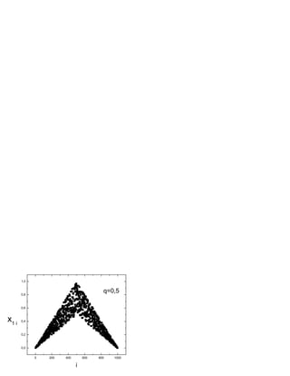
The energy associated to the node i is restricted to the interior of two straight lines of slope ±1
and ±q respectively. In Fig. 1 we can see an example of
the distribution of values around node 1 in a system of
Ei = xij (2) 1000 individuals and q = 0.5. The social correlate of this
j∈νi choice in the distribution of affinity is to privilege closer
neighbors when choosing who to be connected with. One
where νi denotes the neighborhood of i. Finally, we define can imagine a number of examples where this is the case
the global energy of the network, E as follows and clearly, the vicinity or spatial proximity affects the
affinity between two individuals.
N N −1 N
E= Ei = xiˆ
j (3)
i=1 i=1 ˆ i
j∈ν
1.0
where the sum is over the individuals ˆ in νi such that
j
ˆ>i
j 0.8
The choice of the values that conform X is of fun-
damental importance in the development of the inter- 0.6
actions, and therefore in the outcome of the dynam-
ics. Hence, special attention is paid to this feature of x
1 i 0.4
the model resulting in two different approaches, distin-
guished by the characteristics of the (initial) distribution 0.2
of affinities. The first one, namely random distributed, as-
signs to the elements of X random values between 0 and
0.0
1, classified into a certain number of discrete steps. A so-
cial interpretation of this can be made in terms of a case 0 200 400 600 800 1000
when people to whom one would like to be linked, fol-
i
lows no special pattern within the network, and there is
no correlation between the mutual affinity and the phys-
ical or geographical proximity. That means that (initial)
vicinity or popularity plays no role on the affinity de- FIG. 1: Example of the tension values distribution of node 1,
velopment. This could be the case if the system under when N = 1000 and q = 0.5
study consist in individuals with no previous knowledge
of the others or if the index associated to the node is In this case, we want the spatial distribution to af-
for identification purposes only. As a mean to quantify fect the affinity but not to ultimately determine it. This
the initial range of variability of the affinities we allow would be the case if r was a constant number and the
the random distributed variable to adopt only a discrete distribution of affinity would be so that first individuals
set of values (or steps). The extreme cases correspond in every list will be the first neighbors and so on. More-
to those when a) the affinities can tale only two values over, equally distant neighbors would have equal affinity,
5. 3
due to the circular symmetry in the definition of distance. a) Global decision dynamics (GDD)
One can infer, that as in the case of the stable marriage In this case, the changes in the configuration of the
problem, the dynamic of the system will be governed by network are oriented to minimize the global energy E.
the affinity between individuals, in the sense that an in- Since the energy landscape can be extremely complicated
dividual will try to be connected to others in the first most of the times, the system will get trapped in a con-
positions in her/his list. If we consider the case when r figuration associated with a local minimum. The mean
is constant, the final state of the system would necessary individual energies will still be quite high, representing
be a regular network, in which each node is connected a discomfort situation among the individuals. To avoid
to her/his firsts neighbors. To avoid this trivial case we this situation we recur to a scheme based on simulated
have introduced a random distribution for r. Further- annealing [15, 16], therefore allowed changes will have
more, the parameter q will be closely related to how close a non-zero probability of increasing the global energy,
to the trivial case the final configuration will be, reaching which in the end will help to achieve lower value of E.
a complete matching when q = 1. On the other hand, To continue the analogy with the real annealing, we de-
choosing q close to 0 will lead the system to be closer to a fine a temperature T , which will be responsible for the
random network. In other words, q (or even better 1/q) fluctuations in the global energy. The process starts with
can be considered as an order parameter of the network. an ordered network at a certain initial T . At each time
All these vague concepts regarding the final state of the step, a node and one of its links are randomly chosen.
system will be formalized after defining the dynamics. The evaluation of the rewiring of the chosen links fol-
lows, by measuring the change in energy involved in this
procedure, namely ∆E. The change is accepted with
B. Network Dynamics probability pa with
1 if ∆E < 0
Once the affinities list has been assigned to each indi- pa = 1 (6)
2 exp( −∆E ) if ∆E > 0
T
vidual we let the social configuration or network evolve.
We start with nodes conforming an initially ordered net- After a certain amount of time steps (each one com-
work and let the dynamics associated to the traditional prising N computational steps), the threshold value T is
marriage problem lead the social structure to a more sta- reduced, and we iterate until the chosen minimum tem-
ble (less energetic) configuration. The governing dynam- perature is achieved. This temperature usually is chosen
ics may be chosen to minimize the individual energy, Eq. to let the system reach a steady state. Since changes in
(2), or the global one, Eq. (3). We will refer to these the network configuration are made taken into consider-
cases respectively as (global dynamics and individual dy- ation the global benefit, we can say that the individuals
namics ). We will show that in all the considered cases are not “selfish” or that they are not in charge of the
the system also achieves a configuration with both lower evolution. If, for example, we break the link (i, j) and
energies. create the link (i, k) the changes in global energy and in
It is important to point out that on this first stage we i’s energy are, respectively
preserve the number of initial links. The process of net- 1
∆E = (xik + xki − xij − xji ) (7)
work rewiring comprises two aspects that must be clearly 2
defined. On one side there is an affinity based probability ∆Ei = xik − xij .
to break an already established link to create a new one.
It is no difficult to imagine a situation in which ∆E¡ 0
On the other hand, we may consider that each individ-
and ∆Ei ¿ 0. In this case, the change is accepted, even
ual has a minimum number of associated links, thus all
though from i’s point of view is not convenient.
the links will have an extreme attached permanently to a
b) Individual decision dynamics 1 (IDD1)
given node. These are what we call one side-fixed edges.
In this case we consider that the individuals make self-
The possibility of no a priori attached links will be also
ish decisions, since only the individual benefit is taken
considered as well.
into account at each change. The mechanism here is very
much the same as the previous case, the only difference
is that instead of using the value ∆E as a threshold we
1. Case 1: One side-fixed edges
take ∆Ei . Thus, we can not call the process a simulated
annealing anymore though the acceptance of changes is
We will start by considering the case when each node made according to the probability pb defined as
has u edges attached to it by one of the extremes, the
connectivity of each node is at least u, and the mean con-
1 if ∆Ei < 0
nectivity is 2u. Mind that this restriction does not imply pb = 1 (8)
exp( −∆Ei ) if ∆Ei > 0
that the edges are directed, since once the evolution has 2 T
finished, the edges are considered undistinguishable. The Even though changes are made in a way to benefit the
further rewiring of a given link can be chosen in terms individual who is making the decision, without regarding
of a global or individual energy minimization rule. Thus what happens with the global energy, it can be seen that
we distinguish between the following two cases E tends to decrease in this process, as shown if Fig. 2 .
6. 4
2. Case 2: Free edges link also drives the system to a steady situation in the
case of IDD1.
c) Individual decision dynamics 2 (IDD2) The absence of this constraints is what lets the system
The reason for this different approach is that we want evolving under the IDD2 scheme not to freeze in a given
deal with a more realistic individual oriented dynamic. configuration. Once in a configuration with a minimum
This time, edges are no longer attached to any node. The energy, the system continues to explore all the available
only restrain in the dynamics is to preserve the number changes leading to other configurations without a change
of link and the connectivity of the underlying network. in the energy. It is now completely possible for a change
Therefore we impose that no node is left without a link, to take place in a way that global energy increases, but
in other words, we do not accept isolated individuals. the individual energy (of a certain node) decreases, being
Though this case is similar to IDD1 with u = 1 tehre are the latter the one governing the dynamics.
some important differences. Again, we proceed within a All the three final states present close values of global
simulated annealing frame, but the way we reconnect the energy, generally differing in less than 10%(see insent in
network in every time step changes. Fig. 2), indicating that though the dynamics may be
The new mechanism goes as follows: we choose a node associated to global or individual decisions, the network
i randomly, and look at every node i is connected to, reaches an ordered state.
choosing the one with lower affinity (higher energy value),
lets say j. Now we choose another node k at random not
50
connected to i, and accept to link i with k (replacing j)
with a probability given by Eq. (8). The main difference
between this dynamics and the previous one, IDD1, is 40 4.5
that here we don’t assign u edges to every node, so when 4.4
it comes to decide which link to cut, the choice does not 4.3
restrict to what we previously called assigned edges, but 30
4.2
to any edge the node has. Furthermore, as the decision
E
4.1
whether to accept a connection or not is taken by only 4.0
20
one of the pair of linked nodes, individuals now have the 3.9
10
-12 -12
1.5x10
-12
2x10
-12
2.5x10
possibility to detach from those undesirable connections.
This balance plays a very important role in self organi- 10
zation.
-4 0
10 10
III. NUMERICAL RESULTS
T
In what follows we will describe the results correspond-
ing to the cases of GDD, IDD1 and IDD2, obtained after
extensive numerical simulations of the described model. FIG. 2: Global energies as a function of temperature for the
Most of the simulations were done with networks of cases GDD (full), IDD1 (dashed), and IDD2(dotted), with
100 individuals, with mean connectivity equal to 4 ( u = q = 0.35 and N = 1000. In the inset we show a detail of the
2). When effects that could be associated to size effects evolution for larger times i.e. smaller T
appeared, we increased the size of the system to confirm
our results. According to the way how matrix X was defined, it is
As said, for GDD we expected the system to achieve apparent that, except in a number of cases that depends
a steady state (hopefully the minimum energy state), on q, individuals will prefer to be connected to their closer
where no more changes take place. Meanwhile in IDD1 neighbors. We wonder what kind of network topology
and IDD2, we thought of the system self organizing in will be the final output of a dynamics dominated by this
a state of stationary global energy, where changes still feature.
take place. However, both for random and neighbor cor- We are interested in knowing whether the dynamics
related distributions of affinity, we found that GDD and of the process can lead to a structure with enhanced
IDD1 achieved steady states, with similar values of the clusterization or not, stressing even more the local or-
final global energy (GDD’s value is slightly smaller). On ganization of an ordered network. We study thus, the
the other hand, IDD2 reaches, as expected, a stationary clustering features of the resulting networks, normaliz-
situation just as the one described above, see Fig. 2. The ing the obtained values to the clustering coefficient of
fact that GDD reaches a steady state is a direct result of an ordered network. Our first observation is that when
how the dynamics is defined. Once the system reaches an considering a randomly distributed affinity the final con-
energy minimum and the temperature is not high enough figuration presents a normalized clustering coefficient Cq
to displace it from there, no more changes can take place. considerable lower than 1, indicating that no apparent lo-
The constraint imposed on one of the extremes of each cal structures are being formed. On the contrary, when
7. 5
considering an affinity correlatively distributed, the clus- a locally compact configuration, with nodes tending to
tering presents a marked non monotonous dependence conform closed groups. When we say closed groups we
with parameter q. In figure 3 we can observe that for do not mean disconnected subgraphs but a nodes highly
large 1/q values (i.e. disordered distribution of affinity) connected among them defined a cluster connected to the
the normalized clustering coefficient is low, in accordance rest of the networks through a few number of links.
to what can be expected in a disordered network. How- Another way to analyze the topology of the resulting
ever, when 1/q gets closer to zero, an anomalous behavior networks is by studying the community structure using
takes place, the normalized clustering increases to values an algorithm proposed in [18, 19]. The algorithm allows
greater than 1, meaning that the network clustering is us to evaluate the community structure in a network,
higher than the corresponding value for an ordered net- generating a dendrogram depicting the partition of a net-
work with equal number of nodes and links. Since clus- work into smaller entities. At each step the fusion of two
tering is a measure of connectivity among close neigh- structures is proposed and accepted only if this fusion
bors, the fact that clustering is greater than the refer- lowers a global quantity called modularity. A high mod-
ence value reflects that some kind of closed structures ularity is an evidence of having obtained a good partition
are being formed. Given the correlated distribution, in- of the network under analysis. However, the final result
dividuals tend to favor connections to closed neighbors, does not only depends on the network itself, but also on
but the interplay with a certain degree of disorder intro- the algorithm used to find it. Examples of the resulting
duced by q results, within a certain range of values of q, in dendograms are depicted in Figures 4 a and b. The algo-
a more complex final configuration, with the emergence rithm is finished when the maximal value of modularity
of a more local structure. It is worth mentioning that M is reached. What we observe is that the degree of local
there is a peak in the clustering, meaning that there is a organization is higher when the value of q corresponds to
certain value q presenting optimal clustering. This is a the one presenting the maximum clusterization, depicted
non trivial result that can affect the transport properties in Fig. 3. Both the visible structure of the dendogram
of the network at local levels [17]. and the higher value of modularity reflect this fact.
0.12
0.8
0.10
1.2 0.7
a
0.08
0.6
M
C 0.06 0.5
1.0 1
0.04
0.4
0.3
0.02
0.2
0.8
0.00
0 1 2 3 4 5
10 10 10 10 10 10 0.1
1/q 0.8
C
q 0.6 0.7
b
0.6
M
0.5
0.4 0.4
0.3
0.2
0.2
0.1
i
0.0
0.0
0 1 2 3 4
10 10 10 10 10
1/q
FIG. 4: Examples of the dendograms of the resulting networks
for IDD2, N = 100 and a) q = 0.48, b)q = 10−4
FIG. 3: Normalized clusterization as a function of 1/q, for
the cases GDD (squares), IDD1 (circles), IDD2 (triangles).
In the inset we show the density of nodes c1 for the same
cases. With N = 100, u = 2
IV. CONCLUSIONS
Another quantity that reflects this behavior is what we
denominate C1 nodes, defined as the number of nodes In this work we have presented a model for evolving
c1 with absolute clustering equal to 1. A node being networks where the dynamics of the architecture of the
c1 means that all its neighbors are connected between links is related to the affinity between individuals. This
them. A high mean clustering coefficient might be related aspect associates the model with that of the stable mar-
with a high number of c1 nodes in the network. When riage though in the present case individuals are not form-
analyzing the behavior of C1 as a function of q (Inset of ing couples but groups of affine agents.
Fig. 3) we find that it is similar to the one displayed by One of the most interesting feature is the evolution of
the clustering. It reaches a maximum at a finite value of the clustering coefficient as a function of the disorder of
q. This reinforces the idea that the networks evolves to the initial condition. If we associate the parameter q with
8. 6
a degree of disorder, we can see that the clustering has a systems is preserved.
maximum for an intermediate value of q. The clustering We want to end up by saying that the present work
is an interesting characteristic of the network since it is is only the first stage towards a model of co evolution of
related to local efficiency in transmission of information. the affinity of agents and the topology of the underly-
Previous model of networks only displayed a monotonic ing network. The feedback between this two features in
behavior of this quantity. a more general model can lead to an collection of inter-
On the other hand it is interesting to stress when the esting results with social relevance. But first we wanted
system is driven either by a collective or individual ini- to isolate those aspects related to the network topology
tiative, the results are qualitatively the same. Though as was done in a previous work [20] where it was the
the values of the energy E where higher for the cases re- topology of the network that remained unchanged and
lated to individual dynamics, the overall behavior of the the affinity among agents evolved.
[1] D. Gale, L.S. Shapley, Amer. Math. Monthly 69, 9 [13] D. Gusfield, R.W. Irving, The stable marriage problem:
(1962). structure and algorithms, MIT Press, Cambridge, MA,
[2] Th.M. Nieuwenhuizen, Physica A 252, 178 (1998). 1989.
[3] A. Roth and M. A. Sotomayor, Econometrica 57, 559 [14] D.E. Knuth, Stable marriage and its relation to other
(1989). combinatorial problems, CRM Proceedings & Lecture
[4] A. E. Roth, Math. Oper. Res. 7, 617 (1982). Notes Vol. 10, AMS, 1997.
[5] A. E. Roth, J. of Political Economy, 92, 991 (1984). [15] S. Kirkpatrick, C.D. Gelatt, Jr. , M.P. Vecchi, Science,
[6] G. Demance and D. Gale, Econometrica 53, 873 (1985). 220, 671 (1983).
[7] L. E. Dubins and D. Freeman, Amer. Math. Monthly 88, [16] N. Metropolis, A. Rosenbluth, M. Rosenbluth, A. Teller,
485 (1981). E. Teller, J. Chem. Phys.,21, 1087 (1953).
[8] H. Adachi, Econom. Lett. 68, 43 (2000). [17] V. Latora and M. Marchiori, Phys Rev. E. 87, 19871
[9] M.-J. Omro, M. Dzierzawa, M. Marsili, Y.-C. Zhang, J. (2001)
Physique I France 7 1723 (1997). [18] M. E. J. Newman and M. Girvan, Phys. Rev. E 69,
[10] M. Dzierzawa, M.J. Omro, Physica A 287, 321(2000). 026113 (2004).
[11] G. Caldarelli and A. Capocci. Physica A 300, 325 (2001). [19] M. E. J. Newman, Phys. Rev. E 69, 066133 (2004).
[12] A. Lage-Castellanos and R. Mulet. Physica A 364, 389 [20] M. Kuperman, Phys. Rev. E 73, 046139 (2006).
(2006).