1. The Impact of Homework on Student Achievement∗
Ozkan Eren†
Department of Economics
University of Nevada, Las Vegas
Daniel J. Henderson‡
Department of Economics
State University of New York at Binghamton
January, 2008
Abstract
Utilizing parametric and nonparametric techniques, we assess the role of a heretofore relatively unex-
plored ‘input’ in the educational process, homework, on academic achievement. Our results indicate that
homework is an important determinant of student test scores. Relative to more standard spending related
measures, extra homework has a larger and more significant impact on test scores. However, the effects
are not uniform across different subpopulations. Specifically, we find additional homework to be most ef-
fective for high and low achievers, which is further confirmed by stochastic dominance analysis. Moreover,
the parametric estimates of the educational production function overstate the impact of schooling related
inputs. In all estimates, the homework coefficient from the parametric model maps to the upper deciles
of the nonparametric coefficient distribution and as a by-product the parametric model understates the
percentage of students with negative responses to additional homework.
JEL: C14, I21, I28
Keywords: Generalized Kernel Estimation, Nonparametric, School Inputs, Stochastic Dominance, Stu-
dent Achievement
∗
The authors wish to thank two anonymous referees, Kevin Grier, Qi Li, Essie Maasoumi, Daniel Millimet, Solomon
Polachek, and Jeff Racine for helpful comments which led to an improved version of this paper as well as participants of the
seminars at the University of Oklahoma, Binghamton University and Temple University. The paper also benefited from the
comments of participants at the Winemiller Conference on Methodological Developments of Statistics in the Social Sciences
at the University of Missouri (October, 2006), the North American Summer Meetings of the Econometric Society at Duke
University (June, 2007), and the Western Economic Association International Meetings in Seattle, WA (July, 2007). The
data used in this article can be obtained from the corresponding author upon request.
†
Ozkan Eren, Department of Economics, College of Business, University of Nevada, Las Vegas, 4505 Maryland Parkway,
Las Vegas, NV 89154-6005, U.S.A. Tel: 1-702-895-3776. Fax 1-702-895-1354 E-mail: ozkan.eren@unlv.edu.
‡
Corresponding author: Daniel J. Henderson, Department of Economics, State University of New York, Binghamton, NY
13902-6000, U.S.A. Tel: 1-607-777-4480. Fax: 1-607-777-2681. E-mail: djhender@binghamton.edu.

2. 1 Introduction
Real expenditures per student in the United States have more than tripled over the last four decades
and that public spending on elementary and secondary education amounts to approximately $200 billion.
Unfortunately, the substantial growth in resources devoted to schools have not been accompanied by
any significant changes in student achievement (Hoxby 1999). Given this discontinuity between educa-
tional expenditures and student achievement, economists have produced a voluminous body of research
attempting to explore the primary influences of student learning. The vast majority of papers in this
area have focused on spending related “inputs” such as class size and teachers’ credentials. With a few
exceptions, these studies conclude that measured school “inputs” have only limited effects on student
outcomes (Hanushek 2003). In light of these pessimistic findings, it is surprising how little work has been
devoted to understanding the impact of other aspects of the educational environment on student achieve-
ment.1 In particular, given parental concerns, policy debates and media interest (e.g., Time Magazine,
25 January 1999), very little research to date has been completed on the role of homework.
We know of two empirical studies that examine the effects of homework on student outcomes. Aksoy
and Link (2000), using the National Educational Longitudinal Study of 1988 (NELS:88), find positive and
significant effects of homework on tenth grade math test scores. However, the authors rely on student
responses regarding the hours of homework, which carries the potential risk of a spurious correlation
since it likely reflects unobserved variation in student ability and motivation. Betts (1997) presents the
only empirical work that, to our knowledge, focuses on the hours of homework assigned by the teacher.
This measure of homework is actually a policy variable, which the school or teacher can control. Using
the Longitudinal Study of American Youth, Betts obtains a substantial effect of homework on math test
scores. Specifically, an extra half hour of math homework per night in grades 7 to 11 is estimated to
advance a student nearly two grade equivalents. Furthermore, in a nonlinear model setting, the author
1
Notable exceptions are Eren and Millimet (2007), Figlio and Lucas (2003) and Fuchs and Wößmann (2007). These
studies examine the impact of other aspects of schooling such as the time structure, grading standards and institutional
factors on student achievement.

3. argues that virtually all students (99.3% of the sample) could benefit from extra homework and thus
math teachers could increase almost all students’ achievement by assigning more homework.
Although the aforementioned papers provide careful and important evidence on the effects of home-
work, there are numerous gaps remaining. First, there may be heterogeneity in the returns to homework.
Theoretical treatments of the topic indicate that the responses to extra homework will depend on stu-
dent’s ability level (see, e.g., Betts 1997 and Neilson 2005). In this respect, the impact of homework
may differ among students. Second, the existing educational production function literature relies mostly
on parametric regression models. Although popular, parametric models require stringent assumptions.
In particular, the errors are generally assumed to come from a specified distribution and the functional
form of the educational production function is given a priori. Since the theory predicts a non-monotonic
relation between homework and student achievement, a parametric specification which fully captures the
true relation may be difficult to find. Further, if the functional form assumption does not hold, the
parametric model will most likely lead to inconsistent estimates.
In order to alleviate some of these potential shortcomings, we adopt a nonparametric approach.
Nonparametric estimation procedures relax the functional form assumptions associated with traditional
parametric regression models and create a tighter fitting regression curve through the data.2 These
procedures do not require assumptions on the distribution of the error nor do they require specific
assumptions on the form of the underlying production function. Furthermore, the procedures generate
unique coefficient estimates for each observation for each variable. This attribute enables us to make
inference regarding heterogeneity in the returns.
Utilizing the above stated techniques and the NELS:88, we reach four striking empirical findings. First,
controlling for teacher’s evaluation of the overall class achievement in the educational production function
is crucial. In the absence of such a control, the schooling “inputs” are overstated. Second, relative to
more standard spending related measures such as class size, extra homework appears to have a larger and
2
Nonparametric estimation has been used in other labor economics domains to avoid restrictive functional form assump-
tions (see, e.g., Henderson et al. 2006 and Kniesner and Li 2002).

4. more significant impact on mathematics achievement. However, the effects are not homogenous across
subpopulations. We find additional homework to be more effective for high and low achievers relative to
average achievers. This is further uniformly confirmed by introducing stochastic dominance techniques
into the examination of returns between groups from a nonparametric regression. Third, in contrast to
time spent on homework, time spent in class is not a significant contributor to math test scores. This may
suggest that learning by doing is a more effective tool for improvement in student achievement. Finally,
the parametric estimates of the educational production function overstate the impact of schooling related
inputs. In particular, both the homework and class size coefficients from the preferred parametric model
map to the upper deciles of the coefficient distribution of the nonparametric estimates. Moreover, the
parametric model understates the percentage of students with negative responses to an additional hour
of homework.
The remainder of the paper is organized as follows: Section 2 provides a short sketch of the theoretical
background. The third section describes the estimation strategy, as well as the statistical tests used in
the paper. Section 4 discusses the data and the fifth section presents the results. Finally, Section 6
concludes.
2 Theoretical Background
To motivate our empirical methodology, we briefly summarize the theoretical models of homework ef-
fectiveness on test scores following Betts (1997) and Neilson (2005). The existing models rest on three
important assumptions: (i) Students have differences in abilities and thus require different amounts of
time to complete the same homework assignment. (ii) Homework is beneficial, at least in small amounts
and (iii) Students are time constrained. In the absence of the third assumption, additional homework
can benefit all students regardless of ability level. However, once the third assumption comes into play,
further homework will only affect those who have not hit their individual time constraint or “give-up”
limit.

5. Formally, let M be the (same) amount of time that each student has available for completing their
homework assignment and let H(ai , HWm ) be the amount of time spent on homework by student i,
which is a function of his/her ability (a) and the number of units of homework (HW ) assigned by teacher
m. Moreover, let f be a production function that transforms the ability of student i and the homework
assigned by teacher m into a test score as T Si = f (ai , HWm ). It is assumed that T S is an increasing
function of a. More homework also leads to higher test scores by assumption (ii) and students who have
higher ability complete their homework assignments more quickly under assumption (iii); dH/da < 0.
In addition to the three assumptions, suppose that each unit of homework takes the same length of
time for a given student (i.e., H is homogeneous of degree one with respect to homework) so that the
most homework a student can do is M/H(a, 1) units. Note that M/H(a, 1) is an increasing function of
ability since the denominator is decreasing in a. Then, for any two random students where the ability of
the first is strictly greater than the second, there exists a level of homework above which the difference
between the test score of the first and second student is nondecreasing for a given M .3 In other words,
when the low able student has reached their time constraint but the high able has not, further homework
only positively affects the high ability student. Therefore, the responses to additional homework will
depend on how far each student is from their individual specific “give-up” limit and the relation between
test scores and homework is non-monotonic.
3 Empirical Methodology
3.1 Parametric Model
We begin our empirical methodology with a parametric specification of the educational production func-
tion as
T Silkm = f (HWm , Wi , Ck , Tm , ξ l , µi , β) + εilkm , (1)
3
See Proposition 2 of Neilson (2005) for the full proof.

6. where, as described above, T S is the test score of student i in school l in class k and HW denotes the
hours of homework assigned by teacher m. The vector W represents individual and family background
characteristics, as well as ex ante achievement (lagged test scores), C is a vector of class inputs and T
is a vector of teacher characteristics. We control for all factors invariant within a given school with the
fixed effect ξ, µ is the endowed ability of student i, β is a vector of parameters to be estimated and ε is
a zero mean, normally distributed error term. We attempt to capture ability (a) with lagged test scores
and a host of variables defined for µ. Our main parameter of interest is the coefficient on homework,
which represents the effect of an additional hour of homework on student test scores.
3.2 Generalized Kernel Estimation
Parametric regression models require one to specify the functional form of the underlying data generating
process prior to estimation. Correctly specified parametric models provide consistent estimates and in-
ference based on such estimates is valid. However, uncertainty exists about the shape of the educational
production function because the theory does not provide a guide as to an appropriate functional form
( Betts 1997, Hanushek 2003, and Todd and Wolpin 2003). There could be nonlinear/non-monotonic
relations as well as interactions among regressors, which standard parametric models may not capture.
Furthermore, typical parametric models do not fully conform to the theoretical model described in sec-
tion 2 since they commonly ignore any information regarding heterogeneity in responses to additional
homework.
Given the potential shortcomings of parametric models, we also estimate a nonparametric version of
(1). To proceed, we utilize Li-Racine Generalized Kernel Estimation (Li and Racine 2004 and Racine
and Li 2004) and express the test score equation as
T Si = θ(xi ) + ei , i = 1, ..., N (2)
where θ(·) is the unknown smooth educational production function, ei is an additive error term and N

7. is the sample size. The covariates of equation (1) are subsumed in xi = [xc , xu , xo ], where xc is a vector
i i i i
of continuous regressors (e.g., hours of homework), xu is a vector of regressors that assume unordered
i
discrete values (e.g., race), and xo is a vector of regressors that assume ordered discrete values (e.g.,
i
parental education).
Taking a first-order Taylor expansion of (2) with respect to xj yields
T Si ≈ θ(xj ) + (xc − xc )β(xj ) + ei ,
i j (3)
¡ θ(xj ) ¢
where β(xj ) is defined as the partial derivative of θ(xj ) with respect to xc . The estimator of δ(xj ) ≡ β(xj )
is given by
  ³ ´ −1
µb ¶ N c − xc
θ(xj ) X  1 xi j 
b j) =
δ(x =  Kh,λu ,λo  ³ 
b
β(xj )   ´ ³ ´³ ´0 
i=1 xc − xc
i j xc − xc xc − xc
i j i j
XN µ ¶
1 ´
× Kh,λu ,λo ³ c T Si , (4)
i=1
xi − xc
j
where Kh,λu ,λo is the commonly used product kernel for mixed data (Li and Racine 2006). b refers to the
h
estimated bandwidth associated with the standard normal kernel for a particular continuous regressor.
bu
Similarly, λ refers to the estimated bandwidth associated with the Aitchison and Aitken’s (1976) kernel
bo
function for unordered categorical data and λ is the estimated bandwidth for the Wang and Van Ryzin
(1981) kernel function for ordered categorical data.
Estimation of the bandwidths (h, λu , λo ) is typically the most salient factor when performing non-
parametric estimation. For example, choosing a very small bandwidth means that there may not be
enough points for smoothing and thus we may get an undersmoothed estimate (low bias, high variance).
On the other hand, choosing a very large bandwidth, we may include too many points and thus get
an oversmoothed estimate (high bias, low variance). This trade-off is a well known dilemma in applied
nonparametric econometrics and thus we resort to automatic determination procedures to estimate the

8. bandwidths. Although there exist many selection methods, one popular procedure (and the one used in
this paper) is that of Least-Squares Cross-Validation. In short, the procedure chooses (h, λu , λo ) which
minimize the least-squares cross-validation function given by
N
1X
CV (h, λu , λo ) = [T Sj − b−j (xj )]2 ,
θ (5)
N
j=1
where b−j (·) is the commonly used leave-one-out estimator of θ(x).4
θ
3.3 Model Selection Criteria
To assess the correct estimation strategy, we utilize the Hsiao et al. (2007) specification test for
mixed categorical and continuous data. The null hypothesis is that the parametric model (f (xi , β))
is correctly specified (H0 : Pr [E(T Si |xi ) = f (xi , β)] = 1) against the alternative that it is not (H1 :
³ ´
Pr [E(T Si |xi ) = f (xi , β)] < 1). The test statistic is based on I ≡ E E (ε|x)2 f (x) , where ε = y −f (x, β).
I is non-negative and equals zero if and only if the null is true. The resulting test statistic is
p
N b
h1 h2 · · · hq I
J= ∼ N (0, 1), (6)
b
σ
where
N N
b 1 X X
I = bibj Kh,λu ,λo ,
εε
N2
i=1 j=1,j6=i
N N
2h1 h2 · · · hq X X 2 2 2
σ2 =
b bi bj Kh,λu ,λo ,
ε ε
N2
i=1 j=1,j6=i
Kh,λu ,λo is the product kernel, and q is the number of continuous regressors. If the null is false, J
diverges to positive infinity. Unfortunately, the asymptotic normal approximation performs poorly in
finite samples and a bootstrap method is generally suggested for approximating the finite sample null
4
c
All bandwidths in this paper are calculated using N °.

9. distribution of the test statistic. This is the approach we take.
3.4 Stochastic Dominance
Nonparametric estimation as described in equation (4) generates unique coefficient estimates for each
observation for each variable. This feature of nonparametric estimation enables us to compare (rank)
the returns for subgroups and thus make inferences about who benefits most from additional homework.
Here we propose using stochastic dominance tests for empirical examination of such comparisons.5 The
comparison of the effectiveness of a policy on different subpopulations based on a particular index (such
as a conditional mean) is highly subjective; different indices may yield substantially different conclusions.
In contrast, finding a stochastic dominance relation provides uniform ranking regarding the impact of the
policy among different groups and offers robust inference.
To proceed, let β (HW ) be the actual effect of an additional hour of homework on test scores unique
to an individual (other regressors can be defined similarly). If there exists distinct known groups within
the sample, we can examine the returns between any two groups, say w and v. Here w and v might refer
to males and females, respectively. Denote β w (HW ) as the effect of an additional hour of homework on
test scores to a specific individual in group w. β v (HW ) is defined similarly. Note that the remaining
covariates are not constrained to be equal across or within groups.
In practice, the actual effect of an additional hour of homework on test scores is unknown, but the
b
nonparametric regression gives us an estimate of this effect. {β w,i (HW )}Nw is a vector of Nw estimates
i=1
b
of β w (HW ) and {β v,i (HW )}Nv is an analogous vector of estimates of β v (HW ). F (β w (HW )) and
i=1
G(β v (HW )) represent the cumulative distribution functions of β w (HW ) and β v (HW ), respectively.
Consider the null hypotheses of interest as
5
For empirical applications of stochastic dominance tests on school quality data see Eren and Millimet (2006) and Maa-
soumi et al. (2005). For an empirical application of stochastic dominance tests on fitted values obtained via nonparametric
regression see Maasoumi et al. (2007).

10. Equality of Distributions :
F (β (HW )) = G(β (HW )) ∀β (HW ) ∈ Ω. (7a)
First Order Stochastic Dominance : F dominates G if
F (β (HW )) ≤ G(β (HW )) ∀β (HW ) ∈ Ω, (7b)
where Ω is the union support for β w (HW ) and β v (HW ) . To test the null hypotheses, we define the
empirical cumulative distribution function for β w (HW ) as
b P
1 Nw b
F (β w (HW )) = 1(β w,i (HW ) ≤ β w (HW )), (8)
Nw i=1
b
where 1 (·) denotes the indicator function and G(β v (HW )) is defined similarly. Next, we define the
following Kolmogorov-Smirnov statistics
TEQ = sup b b
|F (β (HW )) − G(β (HW ))|; (9a)
β(HW )∈Ω
TF SD = sup b b
(F (β (HW )) − G(β (HW ))); (9b)
β(HW )∈Ω
for testing the equality and first order stochastic dominance (FSD) relation, respectively.
Unfortunately, the asymptotic distributions of these nonparametric sample based statistics under the
null are generally unknown because they depend on the underlying distributions of the data. We need to
approximate the empirical distributions of these test statistics to overcome this problem. The strategy
following Abadie (2002) is as follows:
(i) Let T be a generic notation for TEQ and for TF SD . Compute the test statistics T for the orig-
b b b b b b
inal sample of {β w,1 (HW ) , β w,2 (HW ) , . . . , β w,Nw (HW )} and {β v,1 (HW ) , β v,2 (HW ) , . . . , β v,Nv (HW )}.

11. b b b b
(ii) Define the pooled sample as Ω = {β w,1 (HW ) , β w,2 (HW ) , . . . , β w,Nw (HW ) , β v,1 (HW ) ,
b b
β v,2 (HW ) , . . . , β v,Nv (HW )}. Resample Nw + Nv observations with replacement from Ω and
b
call it Ωb . Divide Ωb into two groups to obtain Tb .
(iii) Repeat step (ii) B times.
PB b > T ). Reject the null
(iv) Calculate the p-values of the tests with p-value = B −1 b=1 1(Tb
hypotheses if the p-value is smaller than some significance level α, where α ∈ (0, 1/2).
By resampling from Ω, we approximate the distribution of the test statistics when F (β (HW )) =
G(β (HW )). Note that for (7b), F (β (HW )) = G(β (HW )) represents the least favorable case for the
null hypothesis. This strategy allows us to estimate the supremum of the probability of rejection under
the composite null hypothesis, which is the conventional definition of test size.6
4 Data
The data is obtained from the National Educational Longitudinal Study of 1988 (NELS:88), a large
longitudinal study of eighth grade students conducted by the National Center for Educational Statistics.
The NELS:88 is a stratified sample, which was chosen in two stages. In the first stage, a total of 1032
schools on the basis of school size were selected from a universe of approximately 40,000 schools. In
the second stage, up to 26 students were selected from each of the sample schools based on race and
gender. The original sample contains approximately 25,000 eighth grade students. Follow-up surveys
were administered in 1990, 1992, 1994 and 2000.
To measure academic achievement, students were administered cognitive tests in reading, social sci-
ences, mathematics and science during the spring of the base year (eighth grade), first follow-up (tenth
6
Ideally we would like to reestimate the nonparametric returns within each bootstrap replication to take into account the
uncertainty of the returns. Unfortunately, it could be argued that in doing this we should reestimate the bandwidths for
each bootstrap replication, which would be extremely computationally difficult, if not impossible. Thus, the bootstrapped
p-values most likely differ slightly from their “true” values. This is left for future research. Nonetheless, if we obtain a large
p-value, it is unlikely that accounting for such uncertainty would alter the inference.

12. grade) and second follow-up (twelfth grade). Each of the four grade specific tests contain material ap-
propriate for each grade, but included sufficient overlap from previous grades to permit measurement of
academic growth. Although four test scores are available per student, teacher and class information sets
(discussed below) are only available for two subjects per student.
We utilize tenth grade math test scores as our dependent variable in light of the findings of Grogger
and Eide (1995) and Murnane et al. (1995).7 These studies find a substantial impact of mathematics
achievement on postsecondary education, as well as on earnings. Our variable of interest is the hours
of homework assigned daily and comes directly from the student’s math teacher reports. This measure
of homework is a policy variable, which the school administrator or the teacher can control. Relying on
hours spent on homework from the student reports is not as accurate and may yield spurious correlations
since it may reflect unobserved variation in student ability and motivation.8
Since researchers interested in the impact of school quality measures are typically (and correctly)
concerned about the potential endogeneity of school quality variables, we utilize a relatively lengthy vector
of student, family, endowed ability, teacher and classroom characteristics. The NELS:88 data enables us
to tie teacher and class-level information directly to individual students and thus circumvents the risk
of measurement error and aggregation bias. Furthermore, we include school fixed effects as described
in equations (1) and (2) to capture differences between schools that may affect student achievement.
Specifically, our estimations control for the following variables:
Individual: gender, race, lagged (eighth grade) math test score;
Family: father’s education, mother’s education, family size, socioeconomic status of the
family;
Endowed Ability: ever held back a grade in school, ever enrolled in a gifted class, math
7
We follow Boozer and Rouse (2001) and Altonji et al. (2005) and utilize item response theory math test scores.
8
Even though hours of homework assigned by the teacher is a superior measure to hours of homework reported by the
student, it is far from being perfect since we only observe the quantity and not the quality of homework. This limitation
suggests directions for future research and data collection.

13. grades from grade 6 to 8;
Teacher: gender, race, age, education;
School: school fixed effects;
Class: class size, number of hours the math class meets weekly, teacher’s evaluation of the
overall class achievement.
Information on individual and family characteristics and endowed ability variables are obtained from
base year survey questionnaires and data pertaining to the math teacher and class comes from the first
follow-up survey. Observations with missing values for any of the variables defined above are dropped. We
further restrict the sample to students who attend public schools. Table 1 reports the weighted summary
statistics of some of the key variables for the 6913 students in the public school math sample and for the
regression sample used for estimation.9 The means and standard deviations in the regression sample are
similar to those obtained when using the full set of potential public school observations. This similarity
provides some assurance that missing values have not distorted our sample.
Prior to continuing, a few comments are warranted related to the issue of endogeneity/validity of
the set of control variables that we utilize. First, common with existing practice in the educational
production function literature, we include lagged (eighth grade) math test scores in our estimations.
Lagged test scores are assumed to provide an important control for ex ante achievement and capture all
previous inputs in the educational production process, giving the results a “value-added” interpretation
(see, e.g., Hanushek 1979, 2005). The value added specification is generally regarded as being better
than the “contemporaneous” specification to obtain consistent estimates of the contemporaneous inputs.
However, as indicated in Todd and Wolpin (2003), the value added specification is highly susceptible to
bias even if the omitted inputs are orthogonal to the included inputs. The problem mainly arises due to the
correlation between lagged test scores and (unobserved) endowed ability. If this potential endogeneity
9
Our regressions do not use weights. Instead we include controls for the variables used in the stratification, see Rose and
Betts (2004) for a similar approach.

14. of lagged test scores is not taken into account, then the resulting bias will not only contaminate the
estimate of lagged test scores but may be transmitted to the estimates of all the contemporaneous input
effects. To this end, we include a host of variables, as mentioned above, to capture the endowed ability
of students. Furthermore, even in the absence of (or along with) the aforementioned endogeneity, the
value added specification may still generate biased estimates if the potential omitted inputs are correlated
with the lagged test scores. Todd and Wolpin (2003) propose the use of within-estimators (i.e., student
fixed effect) in a longitudinal framework or within-family estimators as alternatives to the value added
specification. We investigate whether the within-estimator affects our results in the next section.
Second, the teacher’s evaluation of the class plays a crucial role in our estimations and therefore,
requires extra attention. The teachers surveyed in the NELS:88 are asked to report “which of the
following best describes the achievement level of the students in this class compared with the average
tenth grade student in this school.” Their choice is between four categories: high, average, low and
widely differing. It is important to note that the overall class evaluation is not based on the test scores
since the teacher surveys were administered prior to the student surveys. That being said, given the
subjective nature of the question, we need to verify the quality of this variable. Under the assumption
that measurement error is not dominant, Bertrand and Mullainathan (2001) indicate that subjective
measures can be helpful as control variables in predicting outcomes. In Table 2, we report the summary
statistics of tenth grade math test scores disaggregated by teachers’ evaluations. As seen in the first
column, the mean test scores are highest (lowest) for the high (low) achievement group. Moreover, the
within-class standard deviation (as well as overall standard deviation) displayed in the third column of
Table 2 is largest for the widely differing achievement group. These findings provide some corroborative
evidence for the validity of teachers’ responses in reflecting overall class ability and thus measurement
error may not be a dominant issue.

15. 5 Empirical Results
5.1 Parametric Estimates
Our parametric specifications are presented in Table 3. For all regression estimates, White standard errors
are reported beneath each coefficient. The first column of Table 3 gives a large significant coefficient for
homework. An additional hour of homework is associated with a gain of 4.01 (0.59) points in math
achievement. Given that the mean test score is approximately 52.22, this represents an increase of
slightly below eight percent. However, this model is simplistic in that it does not take into account many
observable variables that are known to affect test scores. In the second column of Table 3, we include
demographic and family characteristics. There is a slight decrease in the homework coefficient.
The third column adds student’s eighth grade math scores, which gives the results a value-added
interpretation. Including the student’s 8th grade math score greatly reduces the homework coefficient
from 3.47 (0.50) to 0.90 (0.21). However, the coefficient is still statistically significant. In order to capture
the potential endogeneity of lagged test scores due to endowed ability, we include the endowed ability
variables in the fourth column of Table 3.10 Doing so reduces the coefficient of homework to 0.77 (0.20)
and a slightly smaller decrease is observed in the eighth grade math score coefficient as well.
An important concern regarding the effect of homework and any other school quality variables is that
schools may differ in both observable and unobservable dimensions. If school traits are correlated with
homework or other inputs, then it is likely that the coefficients will be biased. Therefore, it is most
prudent to control for any observed and unobserved factors common to all students in a school. We
accomplish this by including the school fixed effects in the fifth column of Table 3. The school dummies
are jointly significant (p-value = 0.00), but the homework coefficient remains practically unchanged.
The sixth and seventh columns of Table 3 add teacher and classroom characteristics (class size and
weekly hours of math class), respectively. Even though the effect of homework is similar in magnitude,
10
The endowed ability variables are jointly significant (p-value = 0.00).

16. two points are noteworthy regarding the selected covariate estimates. First, the class size coefficient is
positive and statistically significant at the 10 percent level in that increasing the number of students in a
math class from the sample average of 23 to 33 will lead to an increase of 0.25 points in math scores. This
finding is consistent and similar in magnitude with Goldhaber and Brewer (1997), who use the NELS:88
to assess the impact of class size on tenth grade math test scores. Second, in contrast to Betts (1997),
we do not find a significant effect of weekly hours of math class on test scores. Moreover, the coefficient
is substantially small in magnitude. It appears that time spent on homework is what matters.
The school fixed effects should capture any factors common to all students in a school, but there
may still be some unobserved ability differences across students within a school. For instance, if the
overall ability of students in a class is high due to nonrandomness in the assignment of students to
classes, then the teacher may increase (decrease) the homework load for students in that particular class.
If this is the case, the homework coefficient is going to be upward (downward) biased. To control for
this possibility, we utilize the teachers’ responses on the overall achievement level of the math class.
Assuming that measurement error is not dominant, this variable may be helpful in predicting test scores.
Regression estimates controlling for class achievement are given in the eighth column of Table 3. The
class achievement variables are jointly significant (p-value = 0.00). The homework coefficient is still
statistically significant, but considerably diminished in magnitude. A similar reduction is observed in the
class size effect as well and it is no longer significant.
Finally, in the last column of Table 3, we test the potential nonlinear effects of homework in the
parametric specification by adding a quadratic term. In this model, the homework squared term is nega-
tive and statistically significant, suggesting evidence for diminishing returns to the amount of homework
assigned. The return to homework becomes zero at around 2.96 hours per day and is negative afterwards.
This corresponds to 0.45% of the sample. At the mean level hours of homework, which is 0.64 per day,
the marginal product (partial effect) of homework is roughly 0.89 (= 1.136 − 2(0.192 ∗ 0.64)).11
11
To check for complementarity in the educational production function, we also tried to include interaction terms between
homework and other schooling inputs (class and teacher characteristics) one at a time. In no case did any of these interactions

17. As noted above, the value added specification relies on the exogeneity assumption of lagged test scores.
If our set of ability variables do not fully capture the endowed ability and/or there are some omitted
inputs correlated with lagged test scores, then our estimates are susceptible to bias. As a robustness
check, we utilize the longitudinal nature of the NELS:88 data for the sample of 6634 observations from
the first and second follow-up surveys and run a student fixed effect model, assuming that the impact
of homework is the same across grades, rather than a value added specification.12 The student fixed
effect estimates are 0.96 (0.42) and -0.18 (0.09) for homework and homework squared (the partial effect
of homework evaluated at the mean level of homework is 0.75), respectively and the remaining covariate
estimates are qualitatively similar to those presented in the last column of Table 3 (all estimates are
available upon request).13 In this respect, our value added specification does not seem to be seriously
contaminated by endogeneity of lagged test scores and therefore, we take the quadratic value added model
(column 9) as our preferred parametric specification for the remainder of the paper.
To summarize, our parametric estimates provide four key insights. First, inclusion of the teacher’s
evaluation of class achievement in the regression is crucial. In the absence of such a control, the coefficients
on homework and class size are overstated. We believe that teacher’s assessment of the class purges out
some of the ability differences within the school, as well as represents the teacher’s expectations from the
class and thus alleviates bias arising from the possible endogeneity of homework. Second, in contrast to
time spent on homework, time spent in class is not a significant contributor to math test scores. This may
suggest that learning by doing is a more effective tool for improvement in student achievement. Third,
compared to more standard spending related measures such as class size, additional homework appears
to have a larger and more significant impact on math test scores. Fourth, hours of homework assigned
exhibit diminishing returns but only 0.45% of the sample respond negatively to additional homework.
become significant at even the 10 percent level.
12
Ideally, we would like to include the eighth grade sample to our student fixed effect estimation as well, however, the
teachers are not asked to report the daily hours of homework assigned in the base year sample.
13
In addition to socioeconomic status and size of the family, teacher and classroom characteristics, the student fixed effect
estimation controls for the following school-grade specific variables: average daily attendance rate, percentage of students
from single parent homes, percentage of students in remedial math and percentage of limited English proficiency students.

18. 5.2 Nonparametric Estimates
Prior to discussing the results, we conduct the Hsiao et al. (2007) specification test based on the as-
sumption that the correct functional form is the last column of Table 3. The preferred parametric model
(ninth column) is strongly rejected (p-value = 0.00); the linear parametric model (eighth column) is also
rejected (p-value = 0.00). These findings raise concerns regarding the functional form assumptions of the
educational production function in the existing school quality literature. Nonparametric models have the
potential to alleviate these concerns since these types of procedures allow for nonlinearities/interactions
in and among all variables.
Turning to the results, Table 4 displays the nonparametric estimates of homework on math test
scores.14 Given the number of parameters (unique coefficient for each student in the sample) obtained
from the Generalized Kernel Estimation procedure, it is tricky to present the results. Unfortunately, no
widely accepted presentation format exists. Therefore, in Table 4, we give the mean estimate, as well
as the estimates at each decile of the coefficient distribution along with their respective bootstrapped
standard errors. The mean nonparametric estimate is positive but statistically insignificant. Looking at
the coefficient distribution, we observe a positive and marginally significant effect for the 60th percentile
and significant effects for the upper three deciles. The squared correlation between the actual and
predicted values of student achievement rises from 0.84 to 0.88 when we switch from the parametric
to nonparametric model. Precision set aside, the parametric estimate at the mean level of homework
obtained from the last column of Table 3 is larger than the corresponding mean of the nonparametric
estimate. More importantly, roughly 25% of the nonparametric estimates are negative. In other words,
more than 25% of the students do not respond positively to additional homework, whereas this ratio is only
0.45% of the sample from the parametric model. Table A1 in the Appendix displays the sample statistics
for those with negative homework coefficients. The most interesting pattern, when we compare it with
14
For all nonparametric estimates, we control for individual, family, endowed ability, teacher and classroom characteristics
as well as school fixed effects.

19. the regression sample, is observed in the overall class achievement. Students with negative coefficients
are intensified in classes, which the teacher evaluates as average. We further analyze this point in the
next sub-section.
Table 5 presents the nonparametric estimates of selected covariates. We present the mean, as well
as the nonparametric estimates corresponding to the 25th , 50th and 75th percentiles of the coefficient
distribution (labelled Q1, Q2 and Q3). The results for the eighth grade math scores are in line with the
parametric estimates and are statistically significant throughout the distribution. The class size effect,
however, differs from the parametric estimates. The mean nonparametric estimate indicates a reversal
in the sign of the class size effect. Even though we do obtain primarily negative coefficients, a majority
are insignificant and thus we are unable to draw a definite conclusion. The mean return to time spent
in class is also negative and larger in magnitude than the parametric estimate. In addition, the negative
effect is statistically significant at the first quartile.
In sum, the relaxation of the parametric specification reveals at least three findings. First, at the
mean, the predicted effect of homework from the parametric estimate (0.89) is roughly 1.5 times larger
than the nonparametric estimate (0.59). Second, parametric estimates understate the percentage of
students with negative responses to homework. However, extra homework continues to be significantly
effective for at least 40% of the sample under the nonparametric model. Third, the sign of the (mean)
class size coefficient is reversed from positive to negative.
5.3 Effects of Homework by Achievement Group
Given the concentration of students with negative responses at the average achievement level, we further
explore the impact of homework on subgroups based on the teacher’s evaluation of the class. Note
that, in contrast to the parametric model, we do not need to split the sample and reestimate for each
subgroup because we have already obtained a unique coefficient for homework for each individual in the
nonparametric model. Table 6 displays the mean nonparametric estimate, the impact at each decile of

20. the coefficient distribution, as well as the parametric estimate of homework for each subgroup. In the
parametric specifications, we exclude the homework squared term unless it is significant at the 10 percent
level or better.
The first column of Table 6 presents the results for the high achievement group. The parametric
estimate of homework is significant with a value of 2.25 (0.53) and is higher than the corresponding
90th percentile of the nonparametric coefficient distribution; the mean nonparametric counterpart is 0.83
(0.40) and statistically significant. Thus, the nonparametric model indicates that the parametric model
vastly overstates the homework effect for virtually the entire subsample. In addition, the parametric
model cannot capture the heterogeneity inherent in the model. For instance, the homework effect is more
than twice as large at the 90th percentile (1.79) of the coefficient distribution as it is at the median (0.71).
The second column presents the estimates for the average achievement group. The parametric and
nonparametric estimates are substantially small in magnitude and do not yield any significant effect of
homework on math test scores. Even though the coefficients are insignificant, the nonparametric model
indicates that nearly 40% of the subsample respond negatively to extra homework. This may not be
surprising given that the students with negative responses are intensified in average achievement classes.
For the low achievement group, unlike the first two columns, we include the homework squared
term in the parametric specification. The return to homework becomes zero at around 2.22 hours and is
negative afterwards. This corresponds to roughly 0.42% of the subsample. At the mean level of homework
(0.53 hours per day), the partial effect of homework is 1.78 and is higher than the corresponding 80th
percentile of the nonparametric coefficient distribution. The mean nonparametric estimate is 0.75 (0.41)
and marginally significant. Similar to the first column, the parametric model overstates the homework
effect and moreover, understates the percentage of students with negative responses, which is around 24%
of the subsample based on the nonparametric coefficient distribution.
For completeness, the last column presents the estimates for students in classes with widely differing
ability levels. The coefficients are large in magnitude but are only statistically significant for the upper

21. three deciles of the nonparametric estimates.
Table 7 displays the results for selected covariates for each subgroup. We present the parametric
results, as well as the nonparametric mean estimates and the nonparametric estimates corresponding
to the 25th , 50th and 75th percentiles of the coefficient distribution. Three results emerge. First, the
parametric estimates of eighth grade math scores are similar in magnitude to the mean (median) of the
nonparametric estimates. Second, for three of the subgroups (high, average and widely differing), we
observe predominantly negative but insignificant coefficients for class size. Similar to the full sample
estimates, the parametric models overstate the class size effect. For the low achievement group, however,
the parametric class size effect is positive, significant and lies in the upper extreme tail of the correspond-
ing distribution of nonparametric estimates. Specifically, the parametric estimate, 0.12 (0.06), maps to
roughly the 85th percentile of the nonparametric coefficient distribution. Finally, for the average achieve-
ment group, the nonparametric estimates of time spent in class are negative and statistically significant
at the mean and median.
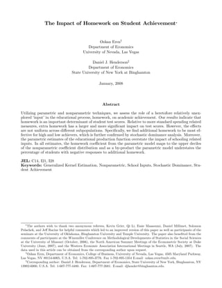
The final set of results are provided in Table 8. We report the p-values associated with the null
hypotheses of equality and FSD for the homework coefficient distributions among the four subgroups.
The corresponding cumulative distribution functions are plotted in Figure 1. For all subgroups, we can
easily reject equality of distributions at conventional confidence levels (p-value = 0.00). In terms of
rankings, homework return for the three subgroups (high, low and widely differing) dominate average
achievers’ returns in the first order sense and further confirm that extra homework is less effective or
may not be effective at all for average achievers. We do not observe FSD between the widely differing
ability group and low or high achievers. There is some evidence of FSD for the return distribution of
high achievers over low achievers, but this evidence is relatively weak.15
As discussed, the theoretical models suggest that homework should positively affect the student’s
achievement up to some limit and then have no effect. In this respect, extra homework leading gains for
15
We also examine the returns to homework for subgroups based on gender and race. The tests do not lead to strong
conclusions for FSD. The results are available upon request.

22. high achievers is not at odds with theory. The mean hours of homework for high achievers is 0.74 (0.40),
but this amount may be far away from the subgroup’s “give-up” limit. The potential puzzle in our results
is that extra homework is not effective for average achievers, despite leading gains for low achievers. One
possibility is that average achievers are at the edge of their maximum effort, whereas low achievers are
below their threshold level. The mean hours of homework are 0.64 (0.36) and 0.53 (0.37) for average and
low achievers, respectively. If the “give-up” level for low achievers is some value greater than 0.53, then
they will benefit from the extra homework. Although this is by no means a definitive explanation for our
findings, it is a plausible explanation.16
6 Conclusion
The stagnation of academic achievement in the United States has given rise to a growing literature seeking
to understand the determinants of student learning. Utilizing parametric and nonparametric techniques,
we assess the impact of a heretofore relatively unexplored “input” in the educational process, homework,
on tenth grade test performance.
Our results indicate that homework is an important determinant of student achievement. Relative
to more standard spending related measures such as class size, extra homework appears to have a larger
and more significant impact on math test scores. However, the effects are not uniform across different
subpopulations. We find additional homework to be most effective for high and low achievers. This
is further confirmed by introducing stochastic dominance techniques into the examination of returns
between groups from a nonparametric regression. In doing so we were able to find that the returns for
both the high and low achievement groups uniformly dominate the returns for the average achievement
group.
Further, in contrast to time spent on homework, time spent in class is not a significant contributor
16
As a robustness check, we also divide the sample based on the eighth grade math score distribution to evaluate homework
effectiveness. Consistent with the teacher’s overall class evaluation, we do not obtain any significant effect for average
achievers. The coefficient estimates for low and high achievers are statistically significant and large in magnitude. These
results are available upon request.

23. to math test scores. This may suggest that learning by doing is a more effective tool for improvement in
student achievement. Finally, parametric estimates of the educational production function overstate the
impact of schooling related inputs and thus raise concerns regarding the commonly used specifications
in the existing literature. Specifically, in all estimates, both the homework and class size coefficients
from the parametric model map to the upper deciles of the nonparametric coefficient distribution and
as a by-product parametric estimates understate the percentage of students with negative responses to
additional homework.

24. References
[1] Abadie, A. (2002), “Bootstrap Tests for Distributional Treatment Effects in Instrumental Variable
Models,” Journal of the American Statistical Association, 97, 284-292.
[2] Aitchison, J. and C.G.G. Aitken (1976), “Multivariate Binary Discrimination by Kernel Method,”
Biometrika, 63, 413-420.
[3] Aksoy, T. and C.R. Link (2000), “A Panel Analysis of Student Mathematics Achievement in the US
in the 1990s: Does Increasing the Amount of Time in Learning Activities Affect Math Achievement?”
Economics of Education Review, 19, 261-277.
[4] Altonji, J., T. Elder and C. Taber (2005), “Selection on Observed and Unobserved Variables: As-
sessing the Effectiveness of Catholic Schools,” Journal of Political Economy, 113, 151-184.
[5] Bertrand, M. and S. Mullainathan (2001), “Do People Mean What They Say? Implications for
Subjective Survey Data,” American Economic Review, 91, 67-72.
[6] Betts, J.R. (1997), “The Role of Homework in Improving School Quality,” Unpublished Manuscript,
Department of Economics, University of California, San Diego.
[7] Boozer, M.A. and C. Rouse (2001), “Intraschool Variation in Class Size: Patterns and Implications,”
Journal of Urban Economics, 50, 163-189.
[8] Eren, O. and D.L. Millimet (2007), “Time to Learn? The Organizational Structure of Schools and
Student Achievement,” Empirical Economics, 32, 301-332.
[9] Figlio, D.N. and M.E. Lucas (2003), “Do High Grading Standards Affect Student Performance?”
Journal of Public Economics, 88, 1815-1834.
[10] Fuchs, T. and L. Wößmann (2007), “What Accounts for International Differences in Student Per-
formance? A Re-Examination Using PISA Data,” Empirical Economics, 32, 433-464.

25. [11] Goldhaber, D.B. and J.B. Brewer (1997), “Why Don’t Schools and Teachers Seem to Matter? As-
sessing the Impact of Unobservables on Educational Productivity,” Journal of Human Resource, 32,
505-523.
[12] Grogger, J. and E. Eide (1995), “Changes in College Skills and the Rise in the College Wage Pre-
mium,” Journal of Human Resources, 30, 280-310.
[13] Hanushek, E.A. (1979), “Conceptual and Empirical Issues in the Estimation of Educational Produc-
tion Functions,” Journal of Human Resources, 14, 351-388.
[14] ––—. (2003), “The Failure of Input Based Schooling Policies,” Economic Journal, 113, 64-98.
[15] ––—. (2005), “Teachers, Schools and Academic Achievement,” Econometrica, 73, 417-458.
[16] Henderson, D.J., A. Olbrecht and S. Polachek (2006), “Do Former Athletes Earn More at Work? A
Nonparametric Assessment,” Journal of Human Resources, 41, 558-577.
[17] Hoxby, C.M. (1999), “The Productivity of Schools and Other Local Public Goods Producers,” Jour-
nal of Public Economics, 74, 1-30.
[18] Hsiao, C., Q. Li and J. Racine (2007), “A Consistent Model Specification Test with Mixed Categorical
and Continuous Data,” Journal of Econometrics, 140, 802-826.
[19] Kniesner, T.J. and Q. Li (2002), “Nonlinearity in Dynamic Adjustment: Semiparametric Estimation
of Panel Labor Supply,” Empirical Economics, 27, 131-48.
[20] Li, Q. and J. Racine (2004), “Cross-Validated Local Linear Nonparametric Regression,” Statistica
Sinica, 14, 485-512.
[21] ––—. (2006), Nonparametric Econometrics: Theory and Practice, Princeton University Press,
Princeton.
[22] Maasoumi, E., D.L. Millimet and V. Rangaprasad (2005), “Class Size and Educational Policy: Who
Benefits from Smaller Classes?” Econometric Reviews, 24, 333-368.

26. [23] Maasoumi, E., J. Racine and T. Stengos (2007), “Growth and Convergence: A Profile of Distribution
Dynamics and Mobility,” Journal of Econometrics, 136, 483-508.
[24] Murnane, R.J., J.B. Willett and F. Levy (1995), “The Growing Importance of Cognitive Skills in
Wage Determination,” Review of Economics and Statistics, 77, 251-266.
c
[25] N °, Nonparametric software by Jeff Racine (http://www.economics.mcmaster.ca/racine/).
[26] Neilson, W. (2005), “Homework and Performance for Time-Constrained Students,” Economics Bul-
letin, 9, 1-6.
[27] Racine, J. and Q. Li (2004), “Nonparametric Estimation of Regression Functions with Both Cate-
gorical and Continuous Data,” Journal of Econometrics, 119, 99-130.
[28] Rose, H. and J.R. Betts (2004), “The Effect of High School Courses on Earnings,” Review of Eco-
nomics and Statistics, 86, 497-513.
[29] Todd, P.E. and K.I. Wolpin (2003), “On the Specification and Estimation of the Production Function
for Cognitive Achievement,” Economic Journal, 113, F3-F33.
[30] Wang, M.C. and J.V. Ryzin (1981), “A Class of Smooth Estimators for Discrete Estimation,” Bio-
metrika, 68, 301-309.

27. Table 1: Sample Statistics of Key Variables
Public School Math Sample Regression Sample
Mean SD Mean SD
10th Grade Math Test Score 51.306 9.850 52.225 9.547
Assigned Daily Hours of Homework 0.643 0.392 0.644 0.381
Weekly Hours of Math Class 3.922 1.033 3.972 1.022
8th Grade Math Test Score 51.488 9.931 52.354 9.901
Mother's Education
High School Dropout 0.133 0.340 0.127 0.333
High School 0.396 0.489 0.418 0.493
Junior College 0.136 0.343 0.139 0.349
College Less Than 4 Years 0.097 0.296 0.091 0.288
College Graduate 0.146 0.353 0.136 0.342
Master Degree 0.069 0.255 0.071 0.257
Ph.D., MD., etc 0.019 0.137 0.015 0.124
Family Size 4.606 1.400 4.565 1.315
Female 0.498 0.500 0.493 0.498
Race
Black 0.117 0.321 0.087 0.281
Hispanic 0.085 0.280 0.068 0.251
Other 0.042 0.202 0.031 0.173
White 0.753 0.499 0.813 0.389
Ever Held Back a Grade (1=Yes) 0.135 0.343 0.134 0.341
Ever Enrolled in a Gifted Class (1=Yes) 0.213 0.409 0.217 0.412
% of Teachers Holding a Graduate Degree 0.508 0.499 0.517 0.499
Teacher's Race
Black 0.050 0.218 0.036 0.186
Hispanic 0.017 0.129 0.016 0.126
Other 0.017 0.131 0.011 0.108
White 0.914 0.279 0.935 0.245
Teacher's Evaluation of the Overall Class Achievement
High Level 0.254 0.435 0.287 0.452
Average Level 0.410 0.491 0.415 0.492
Low Level 0.236 0.424 0.197 0.398
Widely Differing 0.099 0.299 0.100 0.300
Class Size 23.521 7.315 23.442 7.278
Number of Observations 6913 3733
NOTES: Weighted summary statistics are reported. The variables are only a subset of those utilized in the analysis. The remainder are excluded in the interest of brevity. The
full set of sample statistics are available upon request.
26

28. Table 2: Means and Standard Deviations of 10th Grade Math Test Scores by Achievement Levels
Teacher's Evaluation of the Overall Class Achievement Mean SD Within-Class SD
High Achievement 59.769 7.517 3.577
Average Achievement 51.795 8.142 4.177
Low Achievement 43.863 6.618 3.025
Widely Differing 49.995 9.904 4.347
NOTE: Achievement levels are based on teachers' evaluations. See text for further details.
27

29. Table 3: Parametric Estimates of 10th Grade Math Test Scores on Homework
Coefficient
(Standard Error)
(1) (2) (3) (4) (5) (6) (7) (8) (9)
Homework 4.011 3.474 0.905 0.768 0.825 0.921 0.919 0.453 1.136
(0.586) (0.505) (0.213) (0.202) (0.229) (0.229) (0.229) (0.215) (0.429)
Homework Squared … .. … .. … .. … .. … .. … .. … .. … .. -0.192
(0.098)
8th Grade Math Test Score … .. … .. 0.792 0.732 0.725 0.723 0.721 0.661 0.660
(0.008) (0.010) (0.011) (0.011) (0.011) (0.012) (0.012)
Class Size … .. … .. … .. … .. … .. … .. 0.025 0.014 0.014
(0.015) (0.014) (0.014)
Weekly Hours of Math Class … .. … .. … .. … .. … .. … .. 0.009 -0.034 -0.032
(0.112) (0.109) (0.109)
R² 0.027 0.232 0.762 0.778 0.825 0.826 0.826 0.838 0.839
Other Controls:
Demographic and Family Characteristics No Yes Yes Yes Yes Yes Yes Yes Yes
Endowed Ability No No No Yes Yes Yes Yes Yes Yes
School Fixed Effects No No No No Yes Yes Yes Yes Yes
Teacher Characteristics No No No No No Yes Yes Yes Yes
Class Characteristics No No No No No No Yes Yes Yes
Teacher's Evaluation of the Overall Class Achievement No No No No No No No Yes Yes
NOTE: White standard errors are reported in paranthesis. See text for definition of the variables.
28

30. Table 4: Nonparametric Estimates of 10th Grade Math Test Scores on Homework
Coefficient
(Standard Error)
Mean 0.593
(0.523)
10% -0.589
(0.352)
20% -0.165
(0.531)
30% 0.108
(0.543)
40% 0.324
(0.296)
50% 0.513
(0.345)
60% 0.727
(0.398)
70% 0.963
(0.426)
80% 1.308
(0.432)
90% 1.847
(0.567)
R² 0.881
NOTES: Standard errors are obtained via bootstrapping. Estimations control for individual, family, endowed ability
teacher and classroom characteristcs as well as school fixed effects.
Table 5: Quartile Estimates for Selected Covariates
Coefficient
(Standard Error)
Mean Q1 Q2 Q3
8th Grade Math Test Score 0.722 0.658 0.724 0.785
(0.040) (0.023) (0.029) (0.023)
Class Size -0.006 -0.047 -0.016 0.029
(0.036) (0.029) (0.026) (0.085)
Weekly Hours of Math Class -0.229 -0.542 -0.222 0.075
(0.301) (0.230) (0.387) (0.805)
NOTE: Standard errors are obtained via bootstrapping.
29

31. Table 6: Parametric/Nonparametric Estimates of 10th Grade Math Test Scores on Homework by Achievement Level
Coefficient
(Standard Error)
High Achievement Average Achievement Low Achievement Widely Differing
Nonparametric Estimates
Mean 0.832 0.302 0.755 0.610
(0.397) (0.566) (0.413) (1.551)
0.10 0.072 -0.757 -0.608 -0.728
(0.476) (0.486) (1.864) (0.810)
0.20 0.285 -0.454 -0.103 -0.185
(0.728) (0.537) (0.493) (1.194)
0.30 0.413 -0.221 0.137 0.160
(0.364) (0.472) (0.613) (0.942)
0.40 0.553 0.011 0.362 0.488
(0.390) (0.556) (0.950) (0.885)
0.50 0.715 0.231 0.555 0.808
(0.419) (0.735) (0.526) (1.308)
0.60 0.901 0.453 0.794 1.090
(0.447) (0.538) (0.401) (0.895)
0.70 1.100 0.708 1.024 1.522
(0.578) (0.566) (0.599) (0.763)
0.80 1.378 1.019 1.414 1.886
(0.575) (0.648) (0.767) (1.051)
0.90 1.788 1.490 2.042 2.466
(0.489) (0.788) (0.676) (1.006)
Parametric Estimates
Homework 2.254 0.177 2.336 1.023
(0.531) (0.451) (1.587) (1.709)
Homework Squared N/A N/A -0.526 N/A
(0.312)
NOTES: Standard errors are obtained via bootstrapping for the nonparametric estimates and White standard errors are reported for the parametric estimates. Homework squared term
is excluded unless it is significant at 10 % level or better. Estimations control for individual, family, endowed ability, teacher and classroom characteristics as well as school fixed effects.
30

32. Table 7: Quartile Estimates for Selected Covariates by Achievement Level
Coefficient
(Standard Error)
Mean Q1 Q2 Q3 Parametric
High Achievement
8th Grade Math Test Score 0.646 0.593 0.644 0.690 0.587
(0.030) (0.022) (0.031) (0.031) (0.022)
Class Size -0.031 -0.055 -0.034 -0.010 -0.031
(0.036) (0.028) (0.034) (0.034) (0.030)
Weekly Hours of Math Class -0.125 -0.271 -0.099 0.095 -0.078
(0.188) (0.258) (0.211) (0.184) (0.273)
Average Achievement
8th Grade Math Test Score 0.746 0.698 0.743 0.790 0.675
(0.026) (0.023) (0.064) (0.037) (0.021)
Class Size -0.012 -0.047 -0.020 0.008 -0.001
(0.030) (0.034) (0.028) (0.038) (0.027)
Weekly Hours of Math Class -0.510 -0.756 -0.476 -0.253 -0.237
(0.258) (0.503) (0.208) (0.227) (0.200)
Low Achievement
8th Grade Math Test Score 0.752 0.704 0.756 0.809 0.623
(0.050) (0.065) (0.037) (0.034) (0.043)
Class Size 0.054 0.013 0.051 0.090 0.124
(0.046) (0.036) (0.036) (0.035) (0.064)
Weekly Hours of Math Class 0.029 -0.332 -0.007 0.337 0.482
(0.337) (0.371) (0.461) (0.439) (0.360)
Widely Differing
8th Grade Math Test Score 0.786 0.713 0.789 0.855 0.685
(0.044) (0.057) (0.047) (0.038) (0.064)
Class Size -0.021 -0.090 -0.017 0.052 -0.000
(0.060) (0.066) (0.125) (0.011) (0.090)
Weekly Hours of Math Class 0.079 -0.347 0.080 0.539 -0.585
(0.288) (0.419) (0.397) (0.284) (0.730)
NOTE: Standard errors are obtained via bootstrapping for the nonparametric estimates and White standard errors are reported for
the parametric estimates.
31

33. Table 8: Stochastic Dominance Tests of the Coefficient Distributions
Equality of Distributions First Order Stochastic Dominance
p-values p-values
High Achievement/Average Achievement 0.000 0.906
High Achievement/Low Achievement 0.000 0.165
High Achievement/Widely Differing 0.000 0.000
Low Achievement/Average Achievement 0.000 0.961
Low Achievement/Widely Differing 0.000 0.000
Widely Differing/Average Achievement 0.000 0.909
NOTES: Probability values are obtained via bootstrapping. The null hypothesis is rejected if the p-value is smaller than some significance level α (0<α<1/2).
32

34. 1
1
.8
.8
.6
.6
F(.)
F(.)
.4
.4
.2
.2
0
0
-10 -5 0 5 -4 -2 0 2 4 6
Support Support
High Achievers Average Achievers High Achievers Low Achievers
1
1
.8
.8
.6
.6
F(.)
F(.)
.4
.4
.2
.2
0
0
-4 -2 0 2 4 6 -10 -5 0 5 10
Support Support
High Achievers Widely Differ Average Achievers Low Achievers
1
1
.8
.8
.6
.6
F(.)
F(.)
.4
.4
.2
.2
0
0
-10 -5 0 5 10 -4 -2 0 2 4 6
Support Support
Average Achievers Widely Differ Low Achievers Widely Differ
Figure 1: Cumulative Distribution Functions of the Estimated Homework Coefficients from the General-
ized Kernel Estimation Procedure by Achievement Level

35. Appendix :
Table A1: Sample Statistics of Key Variables for Students with Negative Respsonses to Additional Homework
Negative Response Sample
Mean SD
10th Grade Math Test Score 49.586 8.566
Assigned Daily Hours of Homework 0.659 0.470
Weekly Hours of Math Class 3.867 1.114
8th Grade Math Test Score 48.991 8.240
Mother's Education
High School Dropout 0.142 0.349
High School 0.493 0.500
Junior College 0.114 0.318
College Less Than 4 Years 0.078 0.269
College Graduate 0.094 0.292
Master Degree 0.063 0.243
Ph.D., MD., etc 0.012 0.111
Family Size 4.575 1.322
Female 0.537 0.498
Race
Black 0.126 0.332
Hispanic 0.076 0.266
Other 0.023 0.151
White 0.773 0.418
Ever Held Back a Grade (1=Yes) 0.126 0.333
Ever Enrolled in a Gifted Class (1=Yes) 0.154 0.361
% of Teachers Holding a Graduate Degree 0.585 0.492
Teacher's Race
Black 0.061 0.239
Hispanic 0.020 0.142
Other 0.007 0.084
White 0.910 0.285
Teacher's Evaluation of the Overall Class Achievement
High Level 0.097 0.296
Average Level 0.627 0.483
Low Level 0.191 0.393
Widely Differing 0.083 0.277
Class Size 23.891 6.945
Number of Observations 966
NOTES: Weighted summary statistics are reported. The variables listed are only a subset of those utilized in the analysis. The remainder
are excluded in the interest of brevity. The full set of sample statistics are available upon request.
34