1. Designing the Business Process Dimensional Model
Overview
“To arrive at the simple is difficult.”
—Rashid Elisha
This chapter is about the basic concepts of dimensional modeling and the process of designing a business
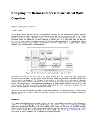
process dimensional model. Designing the dimensional model falls within the central section of the Kimball
Lifecycle, as shown in Figure 2.1. This middle row of the Lifecycle's central section focuses on data, hence
the clever name: the data track. The main objective of the data track is to make sure users get the data
they need to meet ongoing business requirements. The key word in this objective is ongoing: Your goal in
this step is to create a usable, flexible, extensible data model. This model needs to support the full range of
analyses, both now and for the foreseeable future.
Figure 2.1: The dimensional modeling step in the Lifecycle context
The dimensional model is the true heart of the DW/BI system. It is the target for the ETL system, the
structure of the database, and the model behind the user query and reporting experience. Clearly, the
model must be well designed. The first part of this chapter is a brief primer on dimensional modeling,
including an overview of facts, dimensions, the data warehouse bus matrix, and other core concepts. The
second major section of the chapter delves into more detail on several important design techniques, such as
slowly changing dimensions, hierarchies, and bridge tables. Once the basic concepts are in place, the third
section presents a process for building dimensional models.
The fourth part of the chapter describes a dimensional model for the Adventure Works Cycles orders
business process, providing an opportunity to explore several common dimensional modeling issues and
their solutions.
Resources
This chapter describes what a dimensional model is, why it's a useful design technique for a DW/BI system,
and how to go about designing a strong data foundation. You cannot possibly learn everything you need to
know about dimensional modeling in a single chapter—even a long one like this. For additional detailed
guidance on the techniques, including industry case studies, we refer you to The Data Warehouse Toolkit,
Second Edition, Ralph Kimball and Margy Ross (Wiley, 2002). We provide page references for more
information on specific concepts and techniques throughout this chapter.

2. Dimensional Modeling Concepts and Terminology
We approach the modeling process with three primary design goals in mind. We want our models to
accomplish the following:
Present the needed information to users as simply as possible
Return query results to the users as quickly as possible
Provide relevant information that accurately tracks the underlying business processes
Albert Einstein captured the main reason we use the dimensional model when he said, ―Make everything as
simple as possible, but not simpler.‖ As it turns out, simplicity is relative. There is broad agreement in data
warehousing and business intelligence that the dimensional model is the preferred structure for presenting
information to users. The dimensional model is much easier for users to understand than the typical source
system normalized model even though a dimensional model typically contains exactly the same content as a
normalized model. It has far fewer tables, and information is grouped into coherent business categories that
make sense to users. These categories, which we call dimensions, help users navigate the model because
entire categories can be disregarded if they aren't relevant to a particular analysis.
Unfortunately, as simple as possible doesn't mean the model is necessarily simple. The model must reflect
the business, and businesses are complex. If you simplify too much, typically by presenting only aggregated
data, the model loses information that's critical to understanding the business. No matter how you model
data, the intrinsic complexity of the data content is ultimately why most people will use structured reports
and analytic applications to access the DW/BI system.
Achieving our second goal of good performance is a bit more platform‐specific. In the relational
environment, the dimensional model helps query performance because of the denormalization involved in
creating the dimensions. By pre‐joining the various hierarchies and lookup tables, the optimizer considers
fewer join paths and creates fewer intermediate temporary tables. Analytic queries against the SQL Server
relational database generally perform better—often far better—against a dimensional structure than against
a fully normalized structure. At a more fundamental level, the optimizer can recognize the dimensional
model and leverage its structure to dramatically reduce the number of rows it returns. This is known as star
join optimization, and is, of course, an Enterprise Edition feature.
In the Analysis Services OLAP environment, the engine is specifically designed to support dimensional
models. Performance is achieved in large part by pre‐aggregating within and across dimensions.
Achieving the third goal requires a full range of design patterns that allow us to create models that
accurately capture and track the business. Let's start with the basic patterns first. A dimensional model is
made up of a central fact table (or tables) and its associated dimensions. The dimensional model is also
called a star schema because it looks like a star with the fact table in the middle and the dimensions serving
as the points on the star. We stick to the term dimensional model in this book to avoid confusion.
From a relational data modeling perspective, the dimensional model consists of a normalized fact table with
denormalized dimension tables. This section defines the basic components of the dimensional model, facts
and dimensions, along with some of the key concepts involved in handling changes over time.
Facts
Each fact table contains the measurements associated with a specific business process, like taking an order,
displaying a web page, admitting a patient, or handling a customer support request. A record in a fact table
is a measurement event. These events usually have numeric values that quantify the magnitude of the
event, such as quantity ordered, sale amount, or call duration. These numbers are called facts (or measures
in Analysis Services).

3. The primary key to the fact table is usually a multi‐part key made up of a subset of the foreign keys from
each dimension table involved in the business event.
Just the Facts
Most facts are numeric and additive (such as sales amount or unit sales), meaning they can be summed up
across all dimensions. Additivity is important because DW/BI applications seldom retrieve a single fact table
record. User queries generally select hundreds or thousands of records at a time and add them up. A simple
query for sales by month for the last year returns only 12 rows in the answer set, but it may sum up across
hundreds of thousands of rows (or more!). Other facts are semi‐additive (such as market share or account
balance), and still others are non‐additive (such as unit price).
Not all numeric data are facts. Exceptions include discrete descriptive information like package size or
weight (describes a product) or store square footage (describes a store). Generally, these less volatile
numeric values end up as descriptive attributes in dimension tables. Such descriptive information is more
naturally used for constraining a query, rather than being summed in a computation. This distinction is
helpful when deciding whether a data element is part of a dimension or fact.
Some business processes track events without any real measures. If the event happens, we get an entry in
the source system; if not, there is no row. Common examples of this kind of event include employment
activities, such as hiring and firing, and event attendance, such as when a student attends a class. The fact
tables that track these events typically do not have any actual fact measurements, so they're called factless
fact tables. We usually add a column called something like event count that contains the number 1. This
provides users with an easy way to count the number of events by summing the event count fact.
Some facts are derived or computed from other facts, just as a net sale number might be calculated from
gross sales minus sales tax. Some semi‐additive facts can be handled using a derived column that is based
on the context of the query. Month end balance would add up across accounts, but not across date, for
example. The non‐additive unit price example could be addressed by defining it as an average unit price,
which is total amount divided by total quantity. There are several options for dealing with these derived or
computed facts. You can calculate them as part of the ETL process and store them in the fact table, you can
put them in the fact table view definition, or you can include them in the definition of the Analysis Services
database. The only way we find unacceptable is to leave the calculation to the user.
Note Using Analysis Services to calculate computed measures has a significant benefit in that you can define
complex MDX calculations for semi‐additive facts that will automatically calculate correctly based on
the context of each query request.
The Grain
The level of detail contained in the fact table is called the grain. We strongly urge you to build your fact
tables with the lowest level of detail that is possible from the original source—generally this is known as the
atomic level. Atomic fact tables provide complete flexibility to roll up the data to any level of summary
needed across any dimension, now or in the future. You must keep each fact table at a single grain. For
example, it would be confusing and dangerous to have individual sales order line items in the same fact
table as the monthly forecast.
Note Designing your fact tables at the lowest practical level of detail, the atomic level, is a major contributor
to the flexibility of the design.
Fact tables are very efficient. They are highly normalized, storing little redundant data. For most
transaction‐driven organizations, fact tables are also the largest tables in the data warehouse database,
often making up 95 percent or more of the total relational database size. The relational fact table
corresponds to a measure group in Analysis Services.

4. Dimensions
Dimensions are the nouns of the dimensional model, describing the objects that participate in the business,
such as employee, subscriber, publication, customer, physician, vehicle, product, service, author, and store.
Each dimension table joins to all the business processes in which it participates. For example, the product
dimension participates in supplier orders, inventory, shipments, and returns business processes. A single
dimension that is shared across all these processes is called a conformed dimension. We talk more about
conformed dimensions in a bit.
Think about dimensions as tables in a database because that's how you'll implement them. Each table
contains a list of homogeneous entities—products in a manufacturing company, patients in a hospital,
vehicles on auto insurance policies, or customers in just about every organization. Usually, a dimension
includes all occurrences of its entity—all the products the company sells, for example. There is only one
active row for each particular occurrence in the table at any time, and each row has a set of attributes that
identify, describe, define, and classify the occurrence. A product will have a certain size and a standard
weight, and belong to a product group. These sizes and groups have descriptions, like a food product might
come in ―Mini‐Pak‖ or ―Jumbo size.‖ A vehicle is painted a certain color, like ―White,‖ and has a certain
option package, such as the ―Jungle Jim sports utility‖ package (which includes side impact air bags, six‐disc
CD player, DVD system, and simulated leopard skin seats).
Some descriptive attributes in a dimension relate to each other in a hierarchical or one‐to‐many fashion. A
vehicle has a manufacturer, brand, and model (such as GM Chevrolet Silverado, or Toyota Lexus RX Hybrid).
Dimensions often have more than one such embedded hierarchy.
The underlying data structures for most relational transaction systems are designed using a technique
known as normalization. This approach removes redundancies in the data by moving repeating attributes
into their own tables. The physical process of recombining all the attributes of a business object, including
its hierarchies, into a single dimension table is known as denormalization. As we described earlier, this
simplifies the model from a user perspective. It also makes the join paths much simpler for the database
query optimizer than a fully normalized model. The denormalized dimension still presents exactly the same
information and relationships found in the normalized model—nothing is lost from an analytic perspective
except complexity.
You can spot dimensions or their attributes in conversation with the business folks because they are often
the ―by‖ words in a query or report request. For example, a user wants to see sales by month by product.
The natural ways users describe their business should be included in the dimensional model as dimensions
or dimension attributes. This is important because many of the ways users analyze the business are often
not captured in the transaction system. Including these attributes in the warehouse is part of the added
value you can provide.
The Power of Dimensions
Dimensions provide the entry points into the data. Dimensional attributes are used in two primary ways: as
the target for constraints and as the labels on the rows and columns of a report. If the dimensional attribute
exists, you can constrain and label. If it doesn't exist, you simply can't.
Bringing Facts and Dimensions Together
The completed dimensional model has a characteristic appearance, with the fact table in the middle
surrounded by the dimensions. Figure 2.2 shows a simple dimensional model for the classic example: the
retail grocery sales business process. Note that this is one of the business process rows from the retail bus
matrix shown in Figure 1.6 back in Chapter 1. It all ties together if you do it right.

5. Figure 2.2: A basic dimensional model for Retail Grocery Sales
This model allows users across the business to analyze retail sales activity from various perspectives.
Category managers can look at sales by product for different stores and different dates. Store planners can
look at sales by store format or location. Store managers can look at sales by date or cashier. There is
something for everyone in the organization in this dimensional model. While this model is reasonably robust,
a large retail grocer would have a few more dimensions, notably customer, and many more attributes.
In Figure 2.2, fields labeled PK are primary keys. In other words, these fields are the basis of uniqueness for
their tables. In a dimensional model, the primary keys of dimensions are always implemented physically as
single columns. The fields labeled FK are foreign keys, and must always match the corresponding PKs in the
dimensions in order to ensure referential integrity. The field labeled DD is a special degenerate dimension,
which is described later.
Resources
To grasp the concept of dimensions and facts, it's helpful to see examples of dimensional models from a
variety of industries and business processes. The Data Warehouse Toolkit, Second Edition has example
dimensional models from many different industries and business processes, including retail sales, inventory,
procurement, order management, CRM, accounting, HR, financial services, telecommunications and utilities,
transportation, education, health care, e‐commerce, and insurance.

6. The Bus Matrix, Conformed Dimensions, and Drill Across
The idea of re‐using dimensions across multiple business processes is the foundation of the enterprise
DW/BI system and the heart of the Kimball Bus Matrix. In the retail grocery example, a dimension such as
product will be used in both the retail sales and the store inventory dimensional models. Because they are
exactly the same products, both models must use the same dimension with the same keys to reliably
support true, cross‐business process analysis. If the logistics folks at the grocer's headquarters want to
calculate inventory turns, they need to combine data from retail sales and inventory at the product level.
This works only if the two business processes use the exact same product dimension with the same keys;
that is, they use a conformed dimension. Conformed dimensions are the cornerstone of the
enterprise‐enabled DW/BI system. This kind of analysis involving data from more than one business process
is called drill across.
Note The precise technical definition of conformed dimensions is that two dimensions are conformed if they
contain one or more fields with the same names and contents. These ―conformed fields‖ must then be
used as the basis for the drill‐across operation.
Note that this idea of drilling across multiple fact tables and combining the answer sets requires a
front‐end tool capable of supporting this function. A powerful reason to use Analysis Services is that
conformed dimensions are part of the basic architecture of the cube, so its calculation engine smoothly
supports drill across.
Examine the Adventure Works Cycles high‐level bus matrix shown in Figure 2.3. Each row of the bus matrix
represents a business process and defines at least one fact table and its associated dimensions. Often, a row
in the matrix will result in several related fact tables that help track the business process from different
perspectives. The orders business process might have an orders transaction fact table at the line‐item level
and an orders snapshot fact table at the order level. Both of these orders‐based dimensional models belong
to the orders business process. We call this grouping a business process dimensional model. The fully
populated enterprise DW/BI system contains sets of dimensional models that describe all the business
processes in an organization's value chain. As you create the business process dimensional models for each
row in the bus matrix, you end up with a much more detailed version of the matrix. Each dimensional model
has its own row grouped by business process. Order transactions and order snapshot would be separate
rows under the orders business process.

7. Figure 2.3: Adventure Works Cycles high‐level enterprise bus matrix
The bus matrix is the enterprise business intelligence data roadmap. Creating the bus matrix is mandatory
for any enterprise‐wide DW/BI effort. Getting enterprise agreement on conformed dimensions is an
organizational challenge for the data modeler and data steward. Having a single dimension table to describe
the company's products, customers, or facilities means the organization has to agree on how each
dimension table is defined. This includes the list of attributes, attribute names, hierarchies, and the business
rules needed to define and derive each attribute in the table. This is politically hard work, and the effort
grows as a function of the number of employees and divisions. But it is not optional. Conformed dimensions
ensure that you are comparing apples to apples (assuming you are selling apples).
Additional Design Concepts and Techniques
Even though the dimensional modeling concepts we've described are fairly simple, they are applicable to a
wide range of business scenarios. However, there are a few additional dimensional modeling concepts and
techniques that are critical to implementing viable dimensional models. We start this section with a couple of
key concepts: surrogate keys and slowly changing dimensions. Then we look at several techniques for
modeling more complex business situations. Finally, we review the different types of fact tables. We briefly
describe each concept or technique and provide references so you can find more detailed information if you
need it.

8. Surrogate Keys
You will need to create a whole new set of keys in the data warehouse database, separate from the keys in
the transaction source systems. We call these keys surrogate keys, although they are also known as
meaningless keys, substitute keys, non‐natural keys, or artificial keys. A surrogate key is a unique value,
usually an integer, assigned to each row in the dimension. This surrogate key becomes the primary key of
the dimension table and is used to join the dimension to the associated foreign key field in the fact table.
Using surrogate keys in all dimension tables reaps the following benefits (and more):
Surrogate keys help protect the DW/BI system from unexpected administrative changes in the keys
coming from the source system.
Surrogate keys allow the DW/BI system to integrate the same data, such as customer, from
multiple source systems where they have different keys.
Surrogate keys enable you to add rows to dimensions that do not exist in the source system. For
example, the date table might have a ―Date not known‖ row.
Surrogate keys provide the means for tracking changes in dimension attributes over time.
Integer surrogate keys can improve query and processing performance compared to larger
character or GUID keys.
The ability to track changes in dimension attributes over time is reason enough to implement surrogate keys
that are managed by the data warehouse. We've regretted it more than once when we decided not to track
changes in attribute values over time, and later found out the historical values were important to support
certain business analyses. We had to go back and add surrogate keys and re‐create the dimension's change
history. This is not a fun project; we encourage you to do it right the first time. If you use surrogate keys for
all dimensions at the outset, it's easier to change a dimension later so that it tracks history.
The biggest cost of using surrogate keys is the burden it places on the ETL system. Assigning the surrogate
keys to the dimension rows is easy. The real effort lies in mapping those keys into the fact table rows. A fact
row comes to the DW/BI system with its source transaction keys in place. We call the transaction system
key the businesskey (or natural key), although it is usually not business‐like. In order to join these fact rows
to the dimension tables, the ETL system must take each business key in each fact row and look up its
corresponding surrogate key in the appropriate dimension. We call this lookup process the surrogate key
pipeline. Integration Services, used to build the ETL system, provides functionality to support this lookup, as
we describe in Chapter 7.
Resources
The following resources offer additional information about surrogate keys:
The Data Warehouse Toolkit, Second Edition, pages 58–62.
Search http://msdn.microsoft.com using the search string ―surrogate key.‖
Slowly Changing Dimensions
Although we like to think of the attribute values in a dimension as fixed, any attribute can change over time.
In an employee dimension, the date of birth should not change over time (other than error corrections,
which your ETL system should expect). However, other fields, such as the employee's department, might
change several times over the length of a person's employment. Many of these changes are critical to
understanding the dynamics of the business. The ability to track these changes over time is one of the
fundamental reasons for the existence of the DW/BI system.
Almost all dimensions have attributes whose values will change over time. Therefore, you need to be
prepared to deal with a change to the value of any attribute. The techniques we use to manage attribute

9. change in a dimension are part of what we call slowly changing dimensions (SCDs). However, just because
something changes, it doesn't mean that change has significance to the business. The choice of which
dimension attributes you need to track and how you track them is a business decision. The main technique
used to deal with changes the business doesn't care about is called type 1, and the main technique used to
handle changes the business wants to track is called type 2.
How Slow Is Slow?
We call this concept a slowly changing dimension attribute because the attributes that describe a business
entity generally don't change very often. Take customer address, for example. The US Census Bureau did an
in‐depth study of migration patterns (www.census.gov/population/www/pop‐profile/geomob.html), and
found that 16.8 percent of Americans move in a given year, and 62 percent of these moves are within the
same county. If a change in zip code is considered to be a significant business event, a simple customer
dimension with name and address information should generate less than 16.8 percent change rows per
year. If an attribute changes rapidly, causing the dimension to grow at a dramatic rate, this usually indicates
the presence of a business process that should be tracked separately, either as a separate dimension, called
a mini‐dimension, or as a fact table rather than as a dimension attribute.
Handling changes using the type 1 technique overwrites the existing attribute value with the new value. Use
this method if the business users don't care about keeping track of historical values when the value of an
attribute changes. The type 1 change does not preserve the attribute value that was in place at the time a
historical transaction occurred. For example, the Adventure Works customer dimension has an attribute for
commute distance. Using type 1, when a customer moves, their old commute distance is overwritten with
the new value. The old value is gone. All purchases, including purchases made prior to the change, will be
associated with the new value for commute distance.
If you need to track the history of attribute changes, use the type 2 technique. Type 2 change tracking is a
powerful method for capturing the attribute values that were in effect at a point in time and relating them to
the business events in which they participated. When a change to a type 2 attribute occurs, the ETL process
creates a new row in the dimension table to capture the new values of the changed dimension attribute. The
attributes in the new row are in effect as of the time of the change moving forward. The previously existing
row is marked to show that its attributes were in effect right up until the appearance of the new row.
Using the type 2 technique to track changes to the example commute distance attribute will preserve
history. The ETL system writes a new row to the customer dimension, with a new surrogate key and date
stamps to show when the row came into effect and when it expires. (The system also updates the expiration
date stamp for the old row.) All fact rows moving forward will be assigned the surrogate key for this new
row. All the existing fact rows keep their old customer surrogate key, which joins to the old row. Purchases
made prior to the change will be associated with the commute distance that was in effect when the purchase
was made.
Type 2 change tracking is more work to manage in the ETL system, although it's transparent to the user
queries. Most of the popular ETL tools, including Integration Services, have these techniques built in. The
commute distance example is a good one in terms of its business impact. If a marketing analyst does a
study to understand the relationship between commute distance and bicycle purchasing, type 1 tracking will
yield very different results than type 2. In fact, type 1 will yield incorrect results, but that may not be
apparent to the analyst.
Here's a good guide for deciding if it's worth the effort to use type 2 change tracking for an attribute: Ask
yourself if the data has to be right.
Note A third change tracking technique, called type 3, keeps separate columns for both the old and new
attribute values—sometimes called ―alternate realities.‖ In our experience, type 3 is less common
because it involves changing the physical tables and is not very extensible. If you choose to use type 3
tracking, you will need to add a new type 3 column for every major change, which can lead to a wide
table. The technique is most often used for an organization hierarchy that changes seldom, perhaps

10. annually. Often, only two versions are kept (current and prior).
Resources
The following resources offer additional information about slowly changing dimensions:
The Data Warehouse Toolkit, Second Edition, pages 95–105.
Books Online: A search for ―slowly changing dimension support‖ will return several related topics.
Downloads
You can find a more detailed version of the commute distance example with example data on the book's web
site (kimballgroup.com/html/booksMDWTtools.html).
Dates
Date is the fundamental business dimension across all organizations and industries, although many times a
date table doesn't exist in the operational environment. Analyses that trend across dates or make
comparisons between periods (that is, nearly all business analyses) are best supported by creating and
maintaining a robust date dimension.
Every dimensional DW/BI system has a date (or calendar) dimension, typically with one row for every day
for which you expect to have data in a fact table. Calling it the date dimension emphasizes that its grain is
at the day level rather than time of day. In other words, the Date table will have 365 or 366 rows in it per
year.
Note The date dimension is a good example of a role‐playing dimension. It is common for a date dimension
to be used to represent different dates, such as order date, due date, and ship date. To support users
who will be directly accessing the relational database, you can either define a view for each role named
appropriately (e.g., Order_Date), or define synonyms on the base view of the date dimension. The
synonym approach is simple, but it only allows you to rename the entire table, not the columns within
the table. Reports that can't distinguish between order date and due date can be confusing.
If your users will access the data through Analysis Services only, you don't need to bother with views
or synonyms to handle multiple roles. Analysis Services has built‐in support for the concept of
role‐playing dimensions. As we discuss in Chapter 8, however, the Analysis Services role‐playing
dimensions are akin to creating relational synonyms: You can name the overall dimension role, but not
each column within the dimension role.
We strongly recommend using a surrogate key for date because of the classic problem often faced by
technical people: Sometimes you don't have a date. While we can't help the technical people here, we can
say that transactions often arrive at the data warehouse database without a date because the value in the
source system is missing, unknowable, or the event hasn't happened yet. Surrogate keys on the date
dimension help manage the problem of missing dates. Create a few rows in the date dimension that describe
such events, and assign the appropriate surrogate date key to the fact rows with the missing dates.
In the absence of a surrogate date key, you'll create date dimension members with strange dates such as
1‐Jan‐1900 to mean Unknown and 31‐Dec‐9999 to mean Hasn't happened yet. Overloading the fact dates in
this way isn't the end of the world, but it can confuse users and cause erroneous results.
The date dimension surrogate key has one slight deviation from the rule. Where other surrogate keys are
usually a meaningless sequence of integers, it's a good idea to use a meaningful value for the date

11. surrogate key. Specifically, use an integer that corresponds to the date in year‐month‐day order, so
September 22, 2010 would be 20100922. This can lead to more efficient queries against the relational
database. It also makes implementing date‐based partitioning much easier, and the partition management
function will be more understandable.
Just to prove that we're not entirely dogmatic and inflexible, we don't always use surrogate keys for dates
that appear as dimension attributes. Generally, if a particular date attribute has business meaning, we use
the date surrogate key. Otherwise we use a date or smalldatetime data type. One way to spot a good
candidate for a date surrogate key is if the attribute's date values fall within the date range of the
organizational calendar, and therefore are all in the Date table.
Resources
The following resources offer additional information about the date dimension:
The Data Warehouse Toolkit, Second Edition, pages 38–41.
Books Online: Search for the topic ―Time Dimensions (SSAS)‖ and related topics.
Degenerate Dimensions
Transaction identifiers often end up as degenerate dimensions without joining to an actual dimension table.
In the retail grocery example, all the individual items you purchase in a trip through the checkout line are
assigned a transaction ID. The transaction ID is not a dimension—it doesn't exist outside the transaction and
it has no descriptive attributes of its own because they've already been handled in separate dimensions. It's
not a fact—it doesn't measure the event in any way, and is not additive. We call attributes such as
transaction ID a degenerate dimension because it's like a dimension without attributes. And because there
are no associated attributes, there is no dimension table. We include it in the fact table because it serves a
purpose from an analytic perspective. You can use it to tie together all the line items in a market basket to
do some interesting data mining, as we discuss in Chapter 13. You can also use it to tie back to the
transaction system if additional orders‐related data is needed. The degenerate dimension is known as a fact
dimension in Analysis Services.
Snowflaking
In simple terms, snowflaking is the practice of connecting lookup tables to fields in the dimension tables. At
the extreme, snowflaking involves re‐normalizing the dimensions to the third normal form level, usually
under the misguided belief that this will improve maintainability, increase flexibility, or save space. We
discourage snowflaking. It makes the model more complex and therefore less usable, and it actually makes
it more difficult to maintain, especially for type 2 slowly changing dimensions.
In a few cases we support the idea of connecting lookup or grouping tables to the dimensions. One of these
cases involves rarely used lookups, as in the example of joining the Date table to the date of birth field in
the customer dimension so we can count customers grouped by their month of birth. We call this
purpose‐specific snowflake table an outrigger table. When you're building your Analysis Services database,
you'll see this same concept referred to as a reference dimension.
Sometimes it's easier to maintain a dimension in the ETL process when it's been partially normalized or
snowflaked. This is especially true if the source data is a mess and you're trying to ensure the dimension
hierarchy is correctly structured. In this case, there's nothing wrong with using the normalized structure in
the ETL application. Just make sure the business users never have to deal with it.
Note Analysis Services can handle snowflaked dimensions and hides the added complexity from the business
users. In the interest of simplicity, we encourage you to fully populate the base dimensions rather than
snowflaking. The one exception is that the Analysis Services build process can go faster for large

12. dimensions, say more than 1 million rows, when the source is snowflaked or fully denormalized in the
ETL staging database. Test it first before you do all the extra work.
Resources
The following resources offer additional information about snowflaking:
The Data Warehouse Toolkit, Second Edition, pages 55–57.
Books Online: Search for the topic ―Dimension Structure‖ and other Books Online topics on
dimensions.
Many‐to‐Many or Multivalued Dimensions
The standard relationship between a dimension table and fact table is called one‐to‐many. This means one
row in the dimension table will join to many rows in the fact table, but one row on the fact table will join to
only one row in the dimension table. This relationship is important because it keeps us from double
counting. Fortunately, in most cases this relationship holds true.
There are two common instances where the real world is more complex than one‐to‐many:
Many‐to‐many between the fact table and a dimension
Many‐to‐many between dimensions
These two instances are essentially the same, except the fact‐to‐dimension version is missing an
intermediate dimension that uniquely describes the group. In both cases, we introduce an intermediate table
called a bridge table that supports the more complex many‐to‐many relationship.
The Many‐to‐Many Relationship Between a Fact and Dimension
A many‐to‐many relationship between a fact table and a dimension occurs when multiple dimension values
can be assigned to a single fact transaction. A common example is when multiple sales people can be
assigned to a given sale. This often happens in complex, big‐ticket sales such as computer systems.
Accurately handling this situation requires creating a bridge table that assembles the sales rep combinations
into groups. Figure 2.4 shows an example of the SalesRepGroup bridge table.

13. Figure 2.4: An example SalesRepGroup bridge table
The ETL process needs to look up the appropriate sales rep group key in the bridge table for the combination
of sales reps in each incoming fact table record, and add a new group if it doesn't exist. Note that the bridge
table in Figure 2.4 introduces a risk of double counting. If we sum dollar sales by sales rep, every sales rep
will get credit for the total sale. For some analyses, this is the right answer, but for others you don't want
any double counting. It's possible to handle this risk by adding a weighting factor column in the bridge table.
The weighting factor is a fractional value that sums to one for each sales rep group. Multiply the weighting
factor and the additive facts to allocate the facts according to the contribution of each individual in the
group.
Note that you might need to add a SalesRepGroupKey table between Orders and SalesRepGroup to support
a true primary key ‐ foreign key relationship. This turns this fact‐to‐dimension instance into a
dimension‐to‐dimension instance.
Many‐to‐Many Between Dimensions
The many‐to‐many relationship between dimensions is an important concept from an analytic point of view.
Most dimensions are not entirely independent of one another. Dimension independence is more of a
continuum than a binary state. At one end of the continuum, the store and product dimensions in a retail
grocery chain are relatively independent, but not entirely. Some store formats don't carry certain products.
Other dimensions are much more closely related, but are difficult to combine into a single dimension
because of their many‐to‐many relationship. In banking, for example, there is a direct relationship between
account and customer, but it's not one‐to‐one. Any given account can have one or more customers as
signatories, and any given customer can have one or more accounts. Banks often view their data from an
account perspective; the MonthAccountSnapshot is a common fact table in financial institutions. The account
focus makes it difficult to view accounts by customer because of the many‐to‐many relationship. One
approach would be to create a CustomerGroup bridge table that joins to the fact table, such as the
SalesRepGroup table in the previous many‐to‐many example. A better approach takes advantage of the
relationship between account and customer, as shown in Figure 2.5.

14. Figure 2.5: An example many‐to‐many bridge table between dimensions
An AccountToCustomer bridge table between the account and customer dimensions can capture the
many‐to‐many relationship with a couple of significant benefits. First, the relationship is already known in
the source system, so creating the bridge table will be easier than the manual build process required for the
SalesRepGroup table. Second, the account‐customer relationship is interesting in its own right. The
AccountToCustomer bridge table allows users to answer questions such as ―What is the average number of
accounts per customer?‖ without joining to any fact table.
Bridge tables are often an indicator of an underlying business process. This is especially true if you must
keep track of changes to bridge tables over time (that is, the relationship itself is type 2). For customers and
accounts, the business process might be called account maintenance, and one of the transactions might be
called ―Add a signatory.‖ If three customers were associated with an account, there would be three Add
transactions for that account in the source system. Usually these transactions and the business processes
they represent are not important enough to track in the DW/BI system with their own fact tables. However,
the relationships and changes they produce are important to analyzing the business. We include them in the
dimensional model as slowly changing dimensions, and in some cases as bridge tables.
Note Analysis Services has functionality to support many‐to‐many dimensions. Analysis Services expects the
same kind of structure that we described in this section. They call the bridge table an intermediate fact
table, which is exactly what it is.
Resources
The following resources offer additional information about many‐to‐many relationships:
The Data Warehouse Toolkit, Second Edition, pages 262–265 for many‐to‐many between fact and
dimension and pages 205–206 for many‐to‐many between dimensions.
Books Online: Enter the search string ―Defining a Many‐to‐Many Relationship‖ for a list of related
Books Online topics.
Hierarchies
Hierarchies are meaningful, standard ways to group the data within a dimension so you can begin with the
big picture and drill down to lower levels to investigate anomalies. Hierarchies are the main paths for
summarizing the data. Common hierarchies include organizational hierarchies, often starting from the
individual person level; geographic hierarchies based on physical location, such as a customer address;
product hierarchies that often correspond to merchandise rollups such as brand and category; and
responsibility hierarchies such as sales territory that assign customers to sales reps (or vice versa). There
are many industry‐related hierarchies, such as the North American Industrial Classification System
(replacement for the Standard Industrial Classification [SIC] code) or the World Health Organization's
International Classification of Diseases—Tenth Modification (ICD‐10).
Simple hierarchies involving a standard one‐to‐many rollup with only a few fixed levels should be
denormalized right into the granular dimension. A four‐level product hierarchy might start with product,
which rolls up to brand, then to subcategory, and finally to category. Each of these levels would simply be
columns in the product dimension table. In fact, this flattening of hierarchies is one of the main design tasks

15. of creating a dimension table. Many organizations will have several different simple hierarchies in a given
dimension to support different analytic requirements.
Of course, not all hierarchies are simple. The challenge for the dimensional modeler is to determine how to
balance the tradeoff between ease of use and flexibility in representing the more difficult hierarchies. There
are at least two common hierarchy challenges: variable‐depth (or ragged hierarchies) and frequently
changing hierarchies. Both of these problems require more complex solutions than simple denormalization.
We briefly describe these solutions here, and refer you to more detailed information in the other Toolkit
books if you should need it.
Variable‐Depth Hierarchies
A good example of the variable‐depth hierarchy is the manufacturing bill of materials that provides the
information needed to build a particular product. In this case, parts can go into products or into intermediate
layers, called sub‐assemblies, which then go into products, also called top assemblies. This layering can go
dozens of levels deep, or more, in a complex product (think about a Boeing 787).
Those of you who were computer science majors may recall writing recursive subroutines and appreciate the
efficiency of recursion for parsing a parent‐child or self‐referencing table. In SQL, this recursive structure is
implemented by simply including a parent key field in the child record that points back to the parent record
in the same table. For example, one of the fields in an Employee table could be the Parent Employee Key (or
Manager Key).
Recursive Capabilities
SQL 99 introduced recursion into the ―official‖ SQL language using the WITH Common Table Expression
syntax. All the major relational database products provide this functionality in some form, including SQL
Server. Unfortunately, recursion isn't a great solution in the relational environment because it requires more
complex SQL than most front‐end tools can handle. Even if the tool can recursively unpack the
self‐referencing dimension relationship, it then must be able to join the resulting dataset to the fact table.
Very few of the query tools are able to generate the SQL required to navigate a parent‐child relationship
together with a dimension‐fact join.
On the other hand, this kind of recursive relationship is easy to build and manage in the Analysis Services
dimensional database. Analysis Services uses different terminology: parent‐child rather than variable‐depth
hierarchies.
The Data Warehouse Toolkit, Second Edition describes a navigation bridge table in Chapter 6 that solves this
problem in the relational world. But this solution is relatively unwieldy to manage and query. Fortunately, we
have some powerful alternatives in SQL Server. Analysis Services has a built‐in understanding of the
parent‐child data structure, and Reporting Services can navigate the parent‐child hierarchy using some of
the advanced properties of the tablix control. If you have variable‐depth hierarchies and expect to use the
relational database for reporting and analysis, it makes sense to include both the parent‐child fields and the
navigation bridge table to meet the needs of various environments.
Frequently Changing Hierarchies
If you need to track changes in the variable‐depth hierarchy over time, your problem becomes more
complex, especially with the parent‐child data structure. Tracking changes, as you recall, requires using a
surrogate key. If someone is promoted, they will get a new row in the table with a new surrogate key. At
that point, everyone who reports to that person will have to have their manager key updated. If manager
key is a type 2 attribute, new rows with new surrogate keys will now need to be generated for these rows. If
there are any folks who report to these people, the changes must ripple down until we reach the bottom of
the org chart. In the worst case, a change to one of the CEO's attributes, such as marital status, causes the

16. CEO to get a new surrogate key. This means the people who report to the CEO will get new surrogate keys,
and so on down the entire hierarchy.
Ultimately, this problem is really about tracking the Human Resources business process. That is, if keeping
track of all the changes that take place in your employee database is a high priority from an analytic point of
view, you need to create a fact table, or a set of fact tables that track these events. Trying to cram all this
event‐based information into a type 2 dimension just doesn't work very well.
Resources
The following resources offer additional information about hierarchies:
The Data Warehouse Toolkit, Second Edition, pages 161–168.
The Data Warehouse Lifecycle Toolkit, Second Edition, pages 268–270.
SQL Server Books Online: Enter the search string ―Attributes and Attribute Hierarchies‖ as a starting
point.
Aggregate Dimensions
You will often have data in the DW/BI system at different levels of granularity. Sometimes it comes to you
that way, as with forecast data that is created at a level higher than the individual product. Other times you
create it yourself to give the users better query performance. There are two ways to aggregate data in the
warehouse, one by entirely removing a dimension, the other by rolling up in a dimension's hierarchy. When
you aggregate using a hierarchy rollup in the relational database, you need to provide a new, shrunken
dimension at this aggregate level. Figure 2.6 shows how the Adventure Works Cycles Product table can be
shrunken to the subcategory level to allow it to join to forecast data that is created at the subcategory level.

17. Figure 2.6: A Subcategory table extracted from the Adventure Works Cycles Product dimension table
Each subcategory includes a mix of color, size, and weight attributes, for example. Therefore, most of the
columns in the Product table do not make sense at the Subcategory level. This results in a much shorter
dimension, hence the common term shrunken dimension.
The keys for aggregate dimensions need to be generated in the ETL process and are not derived from the
base table keys. Records can be added or subtracted from the base table over time and thus there is no
guarantee that a key from the base table can be used in the aggregate dimension.
Note The Analysis Services OLAP engine automatically manages all this behind the scenes.
You can easily hook in a fact table at any level of a dimension. Of course you may still need aggregate
dimensions to support business process metrics (such as forecast), which live at the aggregate level
only.
Resources
The following resource offers additional information about aggregate dimensions:
Kimballgroup.com: Search for the string ―Shrunken Dimensions‖ for an article on aggregate
dimensions. This article also appears on page 539 of the Kimball Group Reader.

18. Junk Dimensions
Many business processes involve several flags or status indicators or types. In a pure dimensional model,
these would each be placed in their own dimension table, which often is just the surrogate key and the
descriptive column, usually with only a few rows. For example, an order transaction might have a payment
type dimension with only three allowed values: ―Credit,‖ ―Cash,‖ or ―Account.‖ Another small order
dimension could be transaction type with only two allowed values: ―Order,‖ or ―Refund.‖ In practice, using a
single table for each small dimension can make the model confusing because there are too many tables.
Worse, it makes the fact table much larger because each small dimension table adds a key column to the
fact table.
The design pattern we apply to this situation is called a junk dimension. A junk dimension is a combination
of the columns of the separate small dimensions into a single table. Transaction type and payment type
could be combined into a single table with two attribute columns: Transaction_Type and Payment_Type. The
resulting TransactionInfo table would only need six rows to hold all possible combinations of payment type
and transaction type. Each fact row would contain a single transaction info key that would join to the
dimension row that holds the correct combination for that fact row.
Note In Analysis Services, each of the different attributes included in the junk dimension becomes a
separate attribute hierarchy. As in the relational data model, the disparate attribute hierarchies would
be grouped together under one dimension, TransactionInfo in our example. You'd hide the bottom
level of the dimension that has the surrogate key representing the intersection of the codes.
Resources
The following resources offer additional information about junk dimensions:
The Data Warehouse Toolkit, Second Edition, pages 117–119.
The Data Warehouse Lifecycle Toolkit, Second Edition, pages 263–265.
Kimballgroup.com: Search for the topic ―Junk Dimensions‖ for a relevant article.
The Three Fact Table Types
There are three fundamental types of fact tables in the DW/BI system: transaction, periodic snapshot, and
accumulating snapshot. Most of what we have described thus far falls into the transaction category.
Transaction fact tables track each transaction as it occurs at a discrete point in time—when the transaction
event occurred. The periodic snapshot fact table captures cumulative performance over specific time
intervals. It aggregates many of the facts across the time period, providing users with a fast way to get
totals. Where periodic snapshots are taken at specific points in time, after the month‐end close, for example,
the accumulating snapshot is constantly updated over time. Accumulating snapshots is particularly valuable
for combining data across several business processes in the value chain. Generally, the design of the
accumulating snapshot includes several date fields to capture the dates when the item in question passes
through each of the business processes or milestones in the value chain. For an orders accumulating
snapshot that captures metrics about the complete life of an order, these dates might include the following:
Order date
Requested ship date
Manufactured date
Actual ship date
Arrival date
Invoice date
Payment received date

19. The accumulating snapshot provides the status of open orders at any point in time and a history of
completed orders just waiting to be scrutinized for interesting metrics.
Note Transaction fact tables are clearly what Analysis Services was designed for. Your Analysis Services
database can accommodate periodic and accumulating snapshots, but you do need to be careful. The
problem is not the model, but the process for updating the data. Snapshot fact tables—particularly
accumulating snapshots—tend to be updated a lot in the ETL process. This is expensive but not
intolerable in the relational database. It's far more expensive for Analysis Services, which doesn't really
support fact table updates at all.
For snapshot facts to work in Analysis Services for even moderate‐sized data sets, you'll need the
Enterprise Edition feature that allows cube partitioning or you'll need to reprocess the entire cube on
every load.
Resources
The following resources offer additional information about the three fact table types:
The Data Warehouse Toolkit, Second Edition, pages 128–130 and 132–135.
The Data Warehouse Lifecycle Toolkit, Second Edition, pages 273–276.
Kimballgroup.com: Enter the search string ―Snapshot Fact Table‖ for articles on the different
fact table types.
Aggregates
Aggregates are precalculated summary tables that serve the primary purpose of improving performance. If
the database engine could instantly roll the data up to the highest level, you wouldn't need aggregate
tables. In fact, precalculating aggregates is one of the two reasons for the existence of OLAP engines such
as Analysis Services (the other reason being more advanced analytic capabilities). SQL Server Analysis
Services can create and manage aggregate tables in the relational platform (called relational OLAP or
ROLAP) or in the OLAP engine. The decision to create aggregate tables in the relational versus OLAP engines
is a tradeoff. If the aggregates are stored in Analysis Services' format, access to the data is limited to tools
that generate MDX. If the aggregates are stored in the relational database, they can be accessed by tools
that generate SQL. If your front‐end tool is adept at generating MDX, using Analysis Services to manage
aggregates has significant advantages. If you must support relational access, especially ad hoc access, you
need to create and manage any aggregate tables needed for performance (using indexed views if possible),
along with the associated aggregate dimensions described earlier.
Note Kimball Group refers to the summary tables as aggregates and the summarization process as
aggregation. SQL Server Analysis Services uses essentially the opposite terminology; in that
environment, an aggregation is the summary table, and aggregates are the rules that define how the
data is rolled up.
In this section, we have covered several of the common design challenges you will typically run up against
in developing a dimensional model. This is not an exhaustive list, but it should be enough to help you
understand the modeling process. If you are charged with the role of data modeler and this is your first
dimensional modeling effort, we again strongly encourage you to continue your education by reading The
Data Warehouse Toolkit, Second Edition.