I will start with a question "why signal can be compressed?" I will then describe quantization, entropy-coding, difference-PCM, and Discrete Cosine Transform (DCT). My main motive will be to illustrate the basic principle rather than to describe the details of each method. Finally I will discuss how these various algorithm combined to get the JPEG standard for image compression. Time permitting, I will comment on various famous theories which lead to JPEG standard.
From the Un-Distinguished Lecture Series (http://ws.cs.ubc.ca/~udls/). The talk was given May 18, 2007.
12. Why can Signals be Compressed?
Because infinite accuracy of signal amplitudes is
(perceptually) irrelevant
24 bit (16777200 different colors) 8 bit (256 different colors)
Compression factor 3
Rate-distortion theory, scalar/vector quantization
-12-
13. Why can Signals be Compressed?
Because signal amplitudes are statistically redundant
Information theory, Huffman coding
-13-
14. Why can Signals be Compressed?
Because signal amplitudes are mutually dependent
250
200
150 “S”
100
50
0 500 1000 1500 2000 2500 3000 3500 4000 4500
200
150 “O”
100
0 1000 2000 3000 4000 5000
Rate-distortion theory, transform coding
-14-
15. Why can Signals be Compressed?
Example of signal with no dependencies between
successive amplitudes (Gaussian uncorrelated noise)
Indeed “noise” compresses badly
-15-
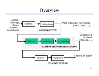
16. System Overview
Analog
capturing PCM encoded or “raw” signal
Sampling Fine Quantization
device (“wav”, “bmp”, …)
(camera,
microphone) A/D CONVERTER
Compressed
bit stream
(mp3, jpg, …)
Transform Quantizer VLC encoding
COMPRESSION/SOURCE CODING
Channel bit stream
Encipher Error protect.
CHANNEL CODING
-16-
17. Quantization
Even Uniform Odd Uniform Q(x)
p(x)
Even Non-uniform Odd Non-uniform
Quantizer level more probable
-17-
20. Run Length Coding
Representing “0 0 0 0 0 0 0 0 1 1 0 0 0 0 0 0 1 1 1 1 1 0 0 ...”
“Runs” : 8 (“zeros”) 2 (“ones”) 6 (“zeros”) 5 (“ones”) ……
The run lengths are also encoded (e.g. with Huffman coding)
Efficient transforms (like DCT) used in compression produce
A lot of “zero” values
And a “few” (significant) non-zero values
Typical symbol sequences to be coded “5 1 0 0 0 0 0 0 0 3 0
0 6 0 0 0 0 1 0 0 0 0 …..”
will be done by {zero-run, non-zero symbol/0} pairs
Here: “{0,5},{0,1},{7,3},{2,6},{4,1},…..”
The pairs will now be assigned a Huffman code
This is used in JPEG
-20-
21. General Compression System
Analog
capturing PCM encoded or “raw” signal
Sampling Fine Quantization
device (“wav”, “bmp”, …)
(camera,
microphone) A/D CONVERTER
Compressed
bit stream
(mp3, jpg, …)
Transform Quantizer VLC encoding
COMPRESSION/SOURCE CODING
Channel bit stream
Encipher Error protect.
CHANNEL CODING
-21-
22. Correlation in Signals - I
Meaningful signals are often highly predictable:
Δx(n)=x(n)-x(n-1)
100
4 250
200
150 0
100
50 100
0 500 1000 1500 2000 2500 3000 3500 4000 4500 500 1000 1500 2000 2500 3000 3500 4000 4500
(Linear) Predictability has something to do with the
autocorrelation function
n
-22-
23. Principle of Differential PCM
x(n) Δx(n) Δx*(n) 001010010
- Q VLC
ˆ
x ( n)
Previous
Predict x(n)
signal values (“past”)
x(n-1), x(n-2), x(n-3), ….
-23-
26. DPCM
Signal to be encoded Prediction difference/error
Predicted signal Reconstructed signal
-26-
27. What Linear Predictor to Use?
Examples:
PCM x( n ) = 0
$
Simple differences x ( n ) = ~ ( n − 1)
$ x
Average last two samples x( n ) = h1 ~ ( n − 1) + h2 ~ ( n − 2)
$ x x
N
x( n) = ∑ hk ~( n − k )
General linear predictor $ x
k =1
-27-
28. DPCM on Images
Same principle as 1-D
Definition of “Past”
and “Future” in Images:
Predictions:
horizontal (scan line)
vertical (column)
2-dimensional
-28-
29. General Compression System
Analog
capturing PCM encoded or “raw” signal
Sampling Fine Quantization
device (“wav”, “bmp”, …)
(camera,
microphone) A/D CONVERTER
Compressed
bit stream
(mp3, jpg, …)
Transform Quantizer VLC encoding
COMPRESSION/SOURCE CODING
Channel bit stream
Encipher Error protect.
CHANNEL CODING
-29-
30. Transform Coding
channel
x(n) x T θ θ$ T-1 $
x $
x(n)
Decorrelating Correlating Inverse
Vectorize
Transform Q Q-1 Transform Vectorize
Which transform used?
-30-
34. Decomposition
N
⎛θ1 ⎞ ⎛ t11 L t1,N ⎞⎛ x1 ⎞
⎜ ⎟ ⎜ , ⎟⎜ ⎟
θk = ∑t
n =1
k ,n xn k = 1, 2 , K , N
θ = ⎜ M ⎟ = ⎜ M O M ⎟⎜ M ⎟ = Tx N
⎜ ⎟ ⎜
⎠
⎜ ⎟
⎝θN⎠ ⎝tN,1 L tN,N⎟⎝ xN⎠ xn = ∑θ
k =1
k t n ,k n = 1, 2 , K , N
N
x = ∑θ
k =1
k t k = θ1 t 1 + θ 2 t 2 + L + θ N t N
t1 0.707
0.25
-0.125 x
0.0
0.0
-0.702
3.165
1.718
2.266
4.516
1.020
0.638
3.377
0.063
-0.2
(Example) t8 -0.025 θ -34-
47. User Controllable Quality
User has control over a “quality parameter” that
runs from 100 (“perfect”) to 0 (“extremely poor”)
Q'
Parameter used to scale
the normalization matrix
6
5
4
3
2
1
0 Q
0 10 20 30 40 50 60 70 80 90 100
Increasing quality
-47-
48. Entropy coding
Runlength coding
Huffman coded then huffman or
arithmetic coding
-48-
51. VLC Coding of AC Coefficients
The (zero run-length, amplitudes) are put into categories
Category AC Coefficient Range
1 -1,1
2 -3,-2,2,3
3 -7,...,-4,4,...,7
4 -15,...,-8,8,...,15
5 -31,...,-16,16,...,31
6 -63,...,-32,32,...,63
7 -127,...,-64,64,...,127
8 -255,...,-128,128,...,255
9 -511,...,-256,256,...,511
10 -1023,...,-512,512,...,1023
The (zero run-length, categories) are Huffman encoded
The sign and offset into a category are FLC encoded
(required #bits = category number)
-51-
52. JPEG AC Huffman Table
Z ero R u n C a teg o ry C o d e len g th C o d ewo rd
0 1 2 00
0 2 2 01
0 3 3 100
0 4 4 1011
0 5 5 11010
0 6 6 111000
0 7 7 1111000
. . . .
. . .
1 1 4 1100
1 2 6 111001
1 3 7 1111001
1 4 9 111110110
. . . .
. . . .
2 1 5 11011
2 2 8 11111000
. . . .
. . . .
3 1 6 111010
3 2 9 111110111
. . . .
. . . .
4 1 6 111011
5 1 7 1111010
6 1 7 1111011
7 1 8 11111001
8 1 8 11111010
9 1 9 111111000
10 1 9 111111001
11 1 9 111111010
. . . .
. . . .
EOB 4 1010
-52-
53. Example - III
The series {1,-2}{0,-1}{0,-1}{0,-1} {2,-1} EOB
now becomes
111001 01/00 0/00 0/00 0/11011 0/1010
Bit rate for AC coefficients in this DCT block 27
bits/64 pixels = 0.42 bit/pixel
-53-