Hanan Einav-Levy Msc Thesis
•
1 j'aime•667 vues

Heat and mass transfer from aerosol bound species, for application in the solar seeded reactor. Supervisors – Prof. Yinon Rudich, Prof. Jacob Karni A method for measuring the sherwood number of aerosols was developed, utilizing an Aerosol mass spectrometer, a thermal denuder, and a differential mobility analyzer and a condensation particle counter. The goal is to use the measured sherwood number for predicting the nusselt number through the heat to mass analogy, as described in the text.

Recommandé
Contenu connexe
Tendances
Tendances (18)
Similaire à Hanan Einav-Levy Msc Thesis
Similaire à Hanan Einav-Levy Msc Thesis (20)
Plus de Hanan E. Levy
Plus de Hanan E. Levy (20)
Dernier
Dernier (20)
Hanan Einav-Levy Msc Thesis
- 1. Thesis for the degree *+"1' (,%1) *#& 1/"-. Master of Science ($./#' 8#)"# Submitted to the Scientific Council of the '! 1$./#, ,9."#' 1!&"# Weizmann Institute of Science ./#' 7#9$" 7"6# Rehovot, Israel '+*!$ ,1"-"4* By 1+# Hanan Einav-Levy $"' -2$. 724 !"#$!" %&' ($'")"*+# ,)# *-.# (/0# 1/$/#' 1$$")$2 ,3$! 4"1$5 (4, *-.# (/0# '+ ,6'!, (!' ,)# *-.#' (4 *-.# 7$- ,$&"'2+- Development of Method for Measuring Mass Transfer Coefficients of Particles and Use of the Mass-Heat Transfer Analogy to Obtain Heat Transfer Coefficients Advisors: :($42# Jacob Karni 8$/"* 7"2$ Yinon Rudich $2*0 -0.$ January 2010 ."!1 3-! - 1
- 2. Abstract ..........................................................................................................................................6 Acknowledgements.........................................................................................................................7 1 Introduction...............................................................................................................................7 1.1 Solar thermal energy...........................................................................................................7 1.2 Convective heat transfer .....................................................................................................8 1.3 The heat to mass transfer analogy.......................................................................................9 1.3.1 Heat and Mass Transfer in the Continuum Regime ......................................................9 1.3.2 The dynamic transfer conditions ................................................................................10 1.3.3 The transition regime.................................................................................................13 2 Research Objectives ................................................................................................................13 3 Experimental Apparatus and Test Results................................................................................14 3.1 Experimental system ........................................................................................................14 3.1.1 Aerosol generation.....................................................................................................16 3.1.2 Coating with High Vapor Pressure Material (Benzo(a)pyrene)...................................16 3.1.3 Controlled evaporation...............................................................................................17 3.1.3.1 Increase of coating material (BaP) ambient vapor pressure..................................18 3.1.3.2 Initial design .......................................................................................................19 3.1.3.3 Final Design........................................................................................................21 3.1.4 Measurement .............................................................................................................22 3.1.5 Experimental Procedure.............................................................................................25 3.1.5.1 Data collection....................................................................................................25 3.1.5.2 Measurement of the side-center temperature correlation matrix...........................26 3.1.5.3 Data analysis procedure ......................................................................................29 3.2 Results .............................................................................................................................31 3.2.1 Mobility and vacuum aerodynamic distributions........................................................31 3.2.2 SMPS measured and AMS mass based final diameter and shape factor......................33 3.2.3 Effects of Residence time ..........................................................................................36 4 Discussion...............................................................................................................................38 4.1 Derivation of the Sherwood number .................................................................................38 4.2 Possible sources of measurement bias...............................................................................40 4.2.1 Coating thickness effect on the Sherwood number .....................................................40 4.2.2 The influence of coating thickness on the calibration ratio RM ...................................42 4.2.3 Possible uneven flow splitting effect on bias..............................................................45 4.3 Error analysis ...................................................................................................................45 4.4 Repeatability ....................................................................................................................47 4.5 Measurement of the Sherwood numbers for suspended nano-particles ..............................47 4.6 The use of the heat to mass analogy for suspended nano-particles.....................................48 4.7 Measurement of fractal soot particles................................................................................49 4.8 Correlation of heat and mass transfer vs. particle size and shape.......................................49 5 Conclusion ..............................................................................................................................50 Appendix A Calculating the Sherwood number from a non isothermal aerosol mass transfer experiment ....................................................................................................................................51 Appendix B Theoretical estimation of the diffusion coefficient of nitrogen-PAH mixture .............52 Appendix C Measuring the desorption energy of PAHs from suspended aerosols..........................53 Bibliography .................................................................................................................................54 2
- 3. List of figures Figure 1: Relevant models for describing transfer dynamics over different ranges of the Knudsen number (Fang 2003) ..............................................................................................................11 Figure 2: Sherwood and Nusselt number prediction for the transition regime ................................12 Figure 3: Experimental system diagram ........................................................................................15 Figure 4: Coating process schematics............................................................................................16 Figure 5: Maximum BaP coating vapor density build up in the Thermal Denuder. ........................20 Figure 6: Final Thermal Denuder (TD) design...............................................................................22 Figure 7: Minimal denuded layer thickness vs. number concentration ...........................................24 Figure 8: HR-AMS mass fragments for BaP coating on PSL.........................................................24 Figure 9: Typical raw data for measurement of BaP evaporation from PSL spheres ......................25 Figure 10: TC probe configuration ................................................................................................26 Figure 11: temperature scan for fast and normal flow rates............................................................28 Figure 12: Calibrating the side thermocouples (T0-T8) versus a central probe (T9) .......................28 Figure 13: Particle size distribution for different extents of evaporation corresponding ................33 Figure 14: Comparison of vacuum aerodynamic distribution for m/z=104 and 252 .......................32 Figure 15: Change in coating thickness due to evaporation............................................................35 Figure 16: Shape factor versus coating thickness...........................................................................35 Figure 17: Effect of residence time. 200 nm PSL sphere, 15 nm thick BaP coating........................36 Figure 18: Effect of residence time. 300 nm PSL sphere 20-25 thick BaP coating .........................37 Figure 19: Effect of residence time. 400 nm PSL sphere 22-30 nm BaP coating............................37 Figure 20: Sherwood number vs. particle diameter........................................................................38 Figure 21: The effect of Coating thickness on the evaporation rate for two limiting cases. ............41 Figure 22: Partial coating scenario schematics...............................................................................42 Figure 23: Calibration ratio of AMS fragment peak mass signal vs. SMPS & CPC mass...............43 Figure 24: Median mobility diameter variations for different PSL sphere diameters......................46 List of tables Table 1 Benzo[a]pyrene (BaP) properties......................................................................................17 Table 2: Typical side-center temperature correlation matrix ..........................................................27 3
- 4. Nomenclature ai, j Temperature L [m] Typical length correlation matrix D [m],[nm] Particle diameter Lmin [nm] Minimum AMS detectable coating thickness Dva [nm] Particle vacuum Loven [m] Thermal Denuder (TD) oven aerodynamic diameter length Dm [nm] Particle mobility ! m '' [Kg s·m ] Mass transfer rate 2 diameter Dm!core [nm] Particle core mobility m0 [ µ g] Residue mass of coating, diameter obtained by Sherwood theory fit Dm!TD [nm] Particle mobility mg [Kg] Gas molecule mass diameter, for aerosols passing through the TD Dm!bypass [nm] Particle mobility mm/z [µg / m 3 ] Mass loading of a single m/z diameter, for aerosols bypassing the TD Df [m 2 s] Binary diffusion mv [Kg] Particle coating molecule mass coefficient DAMS [nm] Equivalent diameter Mw [g / mole] Molecular weight calculated according to AMS and SMPS measurement DSh [nm] Sherwood diameter M coat [g / mole] Coating molecular weight H [KJ / Kg] Latent heat of M AMS [ µ g] Single aerosol coating main evaporation bypass M AMS fragment [m/z] mass, measured by AMS, for aerosols (general – TD M AMS no superscript), or aerosols bypassing the TD (bypass superscript), or going through the TD. h !W m 2 K # Heat transfer M SMPS [ µ g] Single aerosol coating mass, " $ coefficient measured by SMPS, for aerosols M bypass hm [m s] Mass transfer SMPS (general, no superscript), or TD coefficient M SMPS aerosols bypassing the TD, or going through the TD. I [kg / m] Evaporation driving hL Nusselt number Nu = force k ˆ I [ µ g] Normalized n Analogy fit parameter evaporation driving force k [W / mK ] Thermal conductivity No [#/ m 3 ] Molecule number concentration kB [m Kg s K ] Boltzman constant 2 2 N [# m 3 ] Particle number concentration [# cm 3 ] kv [W / mK ] N 2 gas thermal N bypass [#/ cm 3 ] Particle number concentration, conductivity for aerosols bypassing the TD ! Knudsen number Kn = L 4
- 5. p [Pa] Pressure V frac Volume fraction of aerosol ps [Pa] Saturation vapor x o , yo , z o Normalized Cartesian pressure directions pd [Pa] Saturation vapor ! [m 2 s] Thermal diffusivity pressure with Kelvin effect ! Prandtel number !c Energy accommodation Pr = coefficient " q '' !W m 2 # Heat transfer rate ! Relaxation parameter for ai, j " $ correlation matrix calculation Q 3 [m / s] Volumetric flow rate ! o Average gas adiabatic constant R [J / K·mol] The gas constant ! coat [dyne / cm] Coating material surface tension UL Reynolds number !D[m] Coating thickness ReL = ! Roven [m] Thermal Denuder !mAMS"SMPS [ µ g] Single aerosol evaporated (TD) oven radius coating mass, measured by AMS and SMPS RM M SMPS Calibration ratio, for !mSMPS [ µ g] Single aerosol evaporated = aerosols bypassing or coating mass, measured by M AMS passing in the TD SMPS bypass RM M bypass Calibration ratio, for ! [m] Mean free path = SMPS aerosols bypassing the M bypass AMS TD oven S Jayne shape factor ! [m 2 s] Kinematic diffusivity ! Schmidt number !coat [Kg m 3 ] Coating bulk density Sc = Df [g cc] hm L Sherwood number !coat "vapor [Kg m 3 ] Coating vapor density, near the Sh = particle surface, and in the free Df !coat "ambient stream respectively T [K ] Temperature !p [Kg m 3 ] Particle density To Normalized !g [Kg m 3 ] Gas density temperature Tp [K ] Particle temperature !0 [Kg m 3 ] Normalization unit density for Jayne shape factor calculation Tg [K ] Gas temperature ! [!], [K] Lennard Jones potential !, parameters kb Ti (t) [K ] Center of oven ! "m#EV , [ µ g] Repeatability error for !m and temperature ! I "EV I respectively T j (t) [K ] Side of oven ! (Kn) Fuchs correction for mass temperature transfer in transition regime U [m s] Gas velocity ! Dynamic shape factor u o , vo , wo Normalized velocity !o Normalized mass fraction in x o , y o , z o directions 5
- 6. Abstract The use of solar energy for the production of solar fuels is currently studied throughout the world. The first step in the process of solar thermal fuel production is to concentrate the solar flux onto a gas stream. The gas stream used is typically transparent in the solar wavelengths. Therefore, an absorbing medium is employed to absorb the solar flux, and transfer the heat to the gas flow. Recently, Kogan, Kogan & Barak (2005) proposed to use nano-sized black soot particles and the idea was tested in the solar facilities of the Weizmann Institute of Science. The aim of this research is to develop a method for measuring mass transfer from nano- sized particles, such as soot particles, and then obtain heat transfer coefficients through the analogy between mass and heat transfer. The purpose of the mass transfer experiments in this research is to examine the influence of the different experimental parameters on the mass transfer rate, and compare the results to a known theory, thus assessing the efficacy of the measurement method for obtaining mass and heat transfer coefficients. A high resolution Aerodyne aerosol mass spectrometer (AMS) in conjunction with a scanning mobility particle analyzer (SMPS) is used for measuring mass transfer rates of Benzo(a)pyrene (BaP) from polystyrene latex (PSL) spherical particles of different sizes. The experimental apparatus consists of a thermal denuder (TD) with a very uniform and stable temperature profile (±0.2°C over 50 cm). The aerosols were coated by a thin layer of BaP, and then passed through the TD at different speeds and different temperatures. The remaining mass of the BaP was measured by the AMS and was compared to the original mass. A scan of different residence times yields the so-called Sherwood number, which is a dimensionless mass transfer coefficient, describing the ratio of convective to conductive transfer. Experiments were carried out in the transition zone, between the continuum and the kinetic regime where the Sherwood number is expected to decrease monotonically as the particles diameter decreases in this regime. Measurements where performed for 200,300 and 400 nm diameter core PSL spheres, coated by 15-25 nm thick BaP. The results underestimate the theory by 5-25%, with measurement error of ±5-10%, and show the expected trend of increasing Sherwood number with particle diameter. This implies that the proposed method can measure sublimation of thin coatings on high enough number concentrations of aerosols, and the results are similar to pure conduction transport theory, indicating that the process is slow enough and the mass transfer is mainly by conduction. 6
- 7. 9*78; .-&3% -," 98(1 ,.*1"&!/ .*8-$" :&/*:% ;! ;*;&3/:/ %9&7" ;*(5%- ;1/ -3 !&% ,;*:&/*: ;*/9; %*#91!- :/: ;*#91! ;9/%" 0&:!9% "-:% .:/:% ;**#91! .&(; .-&,, ."&9 .% .*/**8% .*/9&'% .(-'&1 &! '#) .9&' .&/*(& ;&!9/ +93/ *"3 %1*98% '&,*9 :* $*/; 0,- .%1*98% ;! .*3-&" .1*! 0,-& ,:/:% ;1*98 -: -#% *,9&! */&(;" .*5&8: -! %32%& %,-&%" .(% ;! 9*"3*& ,./(;* ,:/:% ;1*98 ;! 3-"*: – .( 4*-(/" +9&7 .*-$#" (*5 *8*8-(" :/;:%- &3*7% (2005) 89"& 0#&8 ,0#&8 ,%1&9(!- .&,9$ 9"&3% .9&'% .3$/- 0/7*& 0&,/ -: :/:% -$#/" 0("1 %' 0&*39& ,.(% 4*-(/, .**9)/&11 -: ():% *15/ %2/% 9"3/ .$8/ ;$*$/- %)*: (;5- %;*% %'% 98(/% ;9)/ +*-:%- .( 9"3/- %2/ 9"3/ 0*" %*#&-1!% *"3& ,-"1% (*5% *8*8-( 0&#, ,.*-&2&9! %35:%% ;! 99"- &*% %' 98(/" .**&2*1% -: %9)/% ..(% 9"3/ .$8/ -! &' %$*$/ %2/% 9"3/ "78 -3 (%/*9' ;&9*%/ ,%9&)95/)) ;**&2*1% %)*:" .*9)/95 -: +*93%- +, *"3& ,.**9&$, *8*8-( 9&"3 %3&$* %*9&!*;- ;&&:%- ,.*3&$* .**9&$, .*8*8-(/ .."*"2 '#- .*-&2&9!/ %2/ 9"3/ */$8/ ;$*$/" (;&5: **&2*1% +93/% 8&*$& ;&-*3* ;! ;*-/:( ;&9*"3 9)&8 89&2 "&-*:" (AMS) .*-&2&9!- *$&3** ;&2/ 9)/&9)852 .*8*8-(/ %2/% 9"3/ "78 ;$*$/- &:/*: (SMPS – scanning mobility particle sizer) **&2*1% +93/% .BaP, Benzo[a]pyrene -" .*5&7/ (PSL) 28)- 09*)2*-&5/ .**&:3 .**9&$, +&9! 3)8" $*(! %9&)95/) -*5&95 .3 (Thermal denuder – TD) -*&,/ *&$*! 9&1; --, TD-% +9$ &9"3&% '!& ,BaP -: %8$ %",:" &5&7 .*-&2&9!% .(/"2 50 +9&!- !0.2°C) %;&&:&% BaP-% -: ;9;&1% %2/% ;&/, .;&1&: ;&9&)95/)& ;&1&: %/*9' ;&*&9*%/" ;&*&9*%/ -: .&(; -: %8*92 .SMPS-%& AMS-% *"3 &$$/1: *5, ,;*9&8/% %2/% ;&/,- !&%: ,$&&9:% 952/ ;! -"8- ;1/ -3 %9("1 TD-% -: %9&)95/) %;&!" ;&1&: %/*9' .%*'&5*$" %2/% 9"3/ 0*"- %2/% 9"3/ .$8/ 0*" 2(*% ;! 9!;/% $/*/ 92( 952/ (continuum dynamics) 479% ;(1% .&(; 0*" ,9"3/% .&(;" &37";% .**&2*1% ;$*9* .3 ,%' .&(;" ;*1&)&1&/ ;$9- %5&7/ $&&9:% 952/& ,(kinetic regime) *)1*8% .&(;%& .%9&)95/)& 6(- *!1; .;&!" 8*8-(% -: 9)&8% 15-25 -: .**&5*7 .3 ,9)/&11 400-& 200,300 .*9)8" PSL *8*8-( -3 &:31 ;&$*$/ -: %!*#: .3 %9&!*;% ;! ;/!&;% ,$&&9: 952/" %$*9* &!9% ;&$*$/% .BaP -: 9)/&11 *&2*1% ;)*:& **&2*1% +93/%: %!9/ &' %$*$/ .!5-10% -: %$*$/ ;!*#:& ,5-25% 0*" %2/ 9"3/ -: %(1%%:& ,.*5&7/ .*-&2&9!/ ;&8$ ;&",: -: *&$*! ;$*$/- .*/*!;/ -! %,-:% 9&"3 .*!;%- ;&-&,* %-!, ;&$*$/ 0,-& ,%1&,1 !*% 4! .( 9"3/ !-- ;*)*! ..( 9"3/- %2/ 9"3/ 0*" %*#&-1!% +9$ .(% 9"3/ .$8/
- 8. Acknowledgements I would like to acknowledge Jacob Karni and Yinon Rudich for their priceless advice and support, walking me through the last year and a half of research and education. Yinon sent me to learn first hand on the operation of the AMS, the main and most complicated measurement apparatus, without which I would not have been able to conduct this research in the short time frame I had. He followed my progress closely, making sure I know what I am after at each point. After my first set of experiments I was perplexed by a clear difference between my results and the theory. Jacob went with me through my experimental system step by step, trying to figure out the error, and through his suggestions I found the mistake, and learned to take a pause, and try to look at the problem from a different point of view. For that lesson I am deeply thankful. I would also like to thank the Weizmann institute of science for supporting me with a generous stipend allowing me to dedicate the last 2 years to my Ms.c. studies and research. 1 Introduction 1.1 Solar thermal energy The use of solar energy for the production of electricity and fuels is investigated in industry and academy with the purpose of gradual replacement of non-renewable and polluting energy sources. Solar energy can be utilized in various ways, among them the thermo-solar method, where the sun’s radiation flux is concentrated and used to heat a fluid, which is either used to drive a thermodynamic cycle, which in turn drives a generator and produces electricity (Kribus et al. 1998), or to facilitate a high temperature chemical reaction to produce fuel (Kogan, Kogan, and Barak 2005; Epstein, Ehrensberger, and Yogev 2004). A highly efficient way to facilitate high temperature chemical reactions using particle-laden flow exposed to high concentration of solar flux was proposed and tested (Klein et al. 2007). In this method, a volume of gas, seeded with black soot particles is entrained in a cylinder and exposed to a high concentration of solar flux. The soot particles absorb the flux, heat up, and transfer the heat to the gas by conduction primarily. The experiment conducted by Klein et al. (2007) resulted in an exhaust gas stream with about 200 K higher temperature then the projected values of their model. The most probable reason for this is an under estimation of the conductive heat transfer from the soot particles, since the theory used was based on spherical particles having equivalent surface area to that of the real soot distribution. Thus a system for measuring the real heat transfer coefficient of soot particles, or any particle ensemble, as a function of measurable particle morphology parameters such as the mobility and aerodynamic diameters is desired. 7
- 9. 1.2 Convective heat transfer The process of particle to gas heat transfer is best described by the heat transfer equation q '' = h·(T p ! Tg ) (1) h !W m 2 K # is a heat transfer coefficient, q '' !W m 2 # is the heat flux per particle surface area, " $ " $ T p [K ] and Tg [K ] are the particle surface temperature and free stream gas temperature respectively. The heat transfer coefficient relates the heat flux to the temperature difference, and is a function of the particle morphology; fluid properties and heat transfer mechanism. The heat transfer coefficient can be expressed in a dimensionless form, known as the Nusselt number, relating convective to hL conductive heat transfer across the surface boundary - Nu = where L[m] is a typical length and k k[W / mK ] is the thermal conductivity of the fluid. There are various theoretical and empirical correlations between the Nusselt number and other non-dimensional parameters of the process such as the Reynolds, Grashof and Prandtl numbers (Bird, Warren, and LightFoot 2002) describing the heat transfer of various configurations. Klein et al. (2007) assumed that the relative velocity between each soot particle and the gas stream is zero, and used the pure conduction result for spheres – Nusselt = 2 (Bird, Warren, and LightFoot 2002) ,corrected for the Knudsen number. Since in many cases the particles dimension is relatively close to the mean free path between the gas molecules ![m] , the heat transfer occurs in the transition regime, between continuous transfer dynamics and the kinetic regime, 0.1 < Kn < 10 , ! as defined by the Knudsen number Kn = . In this region the heat transfer coefficient, and L associated Nusselt number, are lower then the continuum solution. Several solutions for the effect of the transition regime on the Nusselt number exist, all built upon the Fuchs boundary layer approach (Filippov and Rosner 2000). To simulate the heat transfer from the soot particles to the gas, Klein et al. (2007) utilized the volume distribution of the soot particle batch used in their tests, as obtained from SEM images, and assumed the Nusselt number relating to each volume segments diameter. The resulting simulations underestimated the experiment by 200 K (~14%). The main reason for this mismatch is assumed to be the heat transfer coefficient used. The particles are not spheres, and consequently the equivalent volume approach was not accurate enough, or may have missed a fundamental difference between the heat transfer from soot agglomerate particles and an equivalent surface area of spheres. Even simpler, this could be the result of the in ability to measure the exact surface area of a soot particle distribution by analyzing 2D SEM pictures. 8
- 10. 1.3 The heat to mass transfer analogy 1.3.1 Heat and Mass Transfer in the Continuum Regime In the continuum regime there is a mathematical-physical equivalence between the energy equation for convective heat transfer, and the species mass transfer equation. The normalized energy equation is (Hong and Song 2007) !T o o !T o o !T o 1 " ! 2T o ! 2T o ! 2T o % uo +v +w = 2 + 2 + (2) !z o ReL Pr $ !x o 2 ' !x o !y o # !y o !z o & UL ! Where the Reynolds number is ReL = , the Prandtl number is Pr = , ! [m 2 s] is the ! " kinematic viscosity, ! [m 2 s] is the thermal diffusivity, U[m s] is a typical velocity, u o , v o , w o are normalized velocities in the normalized directions x o , y o , z o respectively, and T o is the normalized temperature. The normalized mass transfer equation is !" o o !" o o !" o 1 # ! 2" o ! 2" o ! 2" o & u o +v +w = 2 + 2 + (3) ReL Sc % !x o 2 ( !x o !y o !z o $ !y o !z o ' Where ! o is the normalized mass fraction of the transported species in the gas stream, ! Sc = is the Schmidt number and D f [m 2 s] is the diffusion coefficient of the species involved in Df the gas stream. The analogues mass transfer equation to the integral form of the heat transfer equation, (equation (1)), is m '' = hm ·( ! p " !g ) ! (4) ! Where m ''[Kg s·m 2 ] is the mass transfer per unit time and particle surface area; hm [m s] is the mass transfer coefficient; ! p [Kg / m 3 ] and !g [Kg / m 3 ] are the vapor densities of the species being transferred from the particle surface and away from the particles respectively. The mass transfer hm L coefficient is related to the non-dimensional Sherwood number Sh = in the same manner that Df the heat transfer coefficient is related to the Nusselt number. If the Prandtl and Schmidt numbers are the same (which is not common in most fluids), then the Sherwood and Nusselt numbers also equal, for the same flow configuration and boundary conditions. This allows a mass transfer experiment resulting in the Sherwood number to give the Nusselt number by analogy (Hong and Song 2007). Because the Prandtl and Schmidt numbers are not the same in practice, the following approximate relationship is used 9
- 11. n ! Pr $ Nu = Sh # & (5) " Sc % Where n is a fit parameter obtained empirically or by calculation according to the geometry and temperature difference sign (heating or cooling) and is typically between 0.3-0.4 (Incropera and Dewitt 1996; Bird, Warren, and LightFoot 2002). Many expressions for the Nusselt number have been obtained from Sherwood number experiments. For instance, in case of forced convection on a solid sphere Sh = 2 + 0.6 Re1 2 Sc1 3 (6) And by analogy Nu = 2 + 0.6 Re1 2 Pr1 3 (7) The analogy is valid if the following conditions are met: 1. Constant physical properties 2. Small net mass transfer rates 3. No chemical reactions 4. No viscous dissipation heating 5. No absorption or emission of radiant energy 6. No pressure diffusion, thermal diffusion, or forced diffusion 7. Similar boundary conditions In the case of pure diffusion, or pure conduction, the Sherwood and Nusselt numbers are not dependent on the working medium properties (Schmidt or Prandtl numbers) or on flow conditions (Reynolds number). Therefore, the analogy is expected to be even simpler (further discussion on the analogy for suspended aerosols in the transition regime is presented in section 4.6). 1.3.2 The dynamic transfer conditions The objective of the current research is to develop a method for measuring the mass transfer coefficient for nano-size soot and other aerosols, at atmospheric pressure. The measured mass transfer coefficient can be used in conjunction with the heat to mass transfer analogy to give the heat transfer coefficient, which is necessary for further development of the solar thermal seeded particle reactor configuration (see section 2.1 on Solar thermal energy). In the current research, all of the conditions stated in the previous section (top of p. 10) were taken into consideration (see Chapter 4 – Experimental Apparatus and Test Results). The main difference between the heat-mass transfer analogy as previously used and the current one is the dynamic transfer conditions. Soot-particles diameter is typically around 200nm ! 10 µ m , which corresponds to Knudsen numbers of 0.1-10. This is in the transition regime between the continuum 10
- 12. and free molecular regimes (Figure 1). The analogy is known and holds for the continuum regime, but has not been tested for the transition or free molecular regime. The heat and mass transfer equations for the free molecular regime are given by Lees (1965) for instance, for the case of no net flow perpendicular to a surface 4 2kB p $T q fm = ! ! # g [w m 2 ] (8) 3 m g" Tg $x 4 1 $ %p m fm = ! ! # g [Kg m 2 s] (9) 3 2" pg %x Where ![m] is the mean free path of the gas-particle system, defined as $ # + D' !" 2 2 2 ! =1 "No & where [m ] is the effective gas molecule cross-section and D[m] is the % 2 ) ( 4 particle diameter, N o [#/ m 3 ] is the particle number density, mg [Kg] is the gas molecule mass (apparently, it is not specified in the article) and kB [m 2 Kg s 2 K ] the Boltzman constant. Figure 1: Relevant models for describing transfer dynamics over different ranges of the Knudsen number (Fang 2003) For spherical particles the expressions are similar, Filippov and Rosner (2000) give pg ! c kB % # o + 1( q fm = ! ' # o $ 1 * (Tg $ T p ) [W m ] 2 (10) Tg 2 " mg & ) Where ! c is the energy accommodation coefficient (Burke and Hollenbach 1983), and ! o is the average gas adiabatic constant (Filippov and Rosner 2000). Griffin and Loyalka (1994) give the mass transfer to a spherical particle in the free molecular regime: 11
- 13. 8k B m fm = Tg ! ( "g # " p ) [Kg m 2 s] (11) ! mv Where mv [Kg] is the molecular mass of the gas phase molecule. The driving force is similar in both heat and mass transfer expressions (Eq. (10) and (11), respectively), the temperature difference being analogues to the partial pressure (or concentration) difference, but there is no direct correspondence of transport properties coefficients. Instead, these coefficients are related to the pressure, temperature and density of the gas, in different or even opposite ways. The change of the transport properties in the continuum regime with pressure and temperature is also not exactly similar, and this is taken into consideration through the n parameter (Eq. (5)) relating the Schmidt and Prandtel numbers. In the transition regime however, the deviation from the continuum model is similar for both heat and mass transfer, as can be seen in Figure 2, reproducing results for the Nusselt number given by Klein et al. (2007), with Davies results for the Sherwood number shown as well (Eq. (12)). The trend is the same for both non- dimensional numbers, the deviation arising from the models themselves, as can be seen for the large variation for the 4 Nusselt models shown. The Fuchs solution for instance, is the same for both heat and mass transfer in the transition regime (Filippov and Rosner 2000). Analysis of the heat and mass transfer analogy in the transition regime is provided in section 4.6. Figure 2: Sherwood and Nusselt number prediction for the transition regime compared. Nusselt plot reproduced from Klein et al. 2007. Only new addition is the Sherwood number theory by Davies given according to Eq. (12). The Fuchs model (black dashed curve) applies to both mass (Sh) and heat (Nu) transfer as indicated in the figure. 12
- 14. 1.3.3 The transition regime The experiments presented in Chapter 3.2 were conducted in the transition regime; 0.2 < Kn < 0.7 where the dynamics are best described as a combination of a continuum and free molecular dynamics, such as the Fuchs 2-layer approach (Filippov and Rosner 2000): The theory is based on a boundary layer approach. Since there is no general analytical solution of the Boltzmann equation describing gas behavior in the intermediate regime of moderate Knudsen numbers, an interpolation formula is used which is based on the separation of the space outside the particle surface into two parts: Close enough to the surface of the particle (the boundary layer), the conditions are assumed to be collision-less – no collisions between gas molecules, only gas-aerosol interactions are assumed. The boundary layer thickness is typically set to be the same as the gas mean free path. Outside of the boundary layer, the conditions are described by the continuum dynamics. A consistent solution is found for both regimes by ascribing the same heat (or mass) transfer rate at the boundary. Different interpolation formulas exist for mass transfer in the transition regime, as discussed above. Our results are compared to the derivation of Davies (1978) from ((Hinds 1999) p. 288): 2" + D ShKn = 2·! (Kn) = 2· (12) D + 5.33(" 2 D) + 3.42 " Where ! (Kn) is referred to as the Knudsen correction. Multiplying the Knudsen correction by 2, gives the pure diffusion result for Re = 0 (as also predicted by equation (6)). The mean free path is kT calculated according to ! = [m] where p[ pa] is the pressure. In the limiting cases of "d p 2 2 N2 4 1 molecular and continuum regimes, the Sherwood number values are therefore · & 2, 5.33 Kn respectively. Although this derivation is for the case of a light molecule evaporating through a bath gas made out of heavier molecules, which is not our case, using more apparently appropriate derivation, such as Sitarski and Nowakowski (1979) (see Davis 1983) gives very similar results, and so we settled for this simpler derivation. 2 Research Objectives The research objectives are: • Development of an experimental method to measure the evaporative mass transfer from nano aerosol particles in the transition regime • Use the analogy between heat and mass transfer to relate the mass transfer coefficient to the heat transfer coefficient (Eq. (5)). 13
- 15. An important additional objective is the validation of the proposed method – using spherical particles suspended in nitrogen – by experimentally obtaining the theoretically predicted rate of mass transfer, corresponding to each particles size, in the transition regime. 3 Experimental Apparatus and Test Results 3.1 Experimental system A system was designed and built to measure the mass transfer rate from aerosol particles. It is composed of the following components (Figure 3: Experimental system diagram): 1. Aerosol Generation: Create a suspension of monodisperse aerosol – polystyrene latex (PSL) spheres – in nitrogen at atmospheric pressure. 2. Coating of Aerosol with a thin layer of a high vapor pressure material – Benzo(a)pyrene (BaP) 3. Evaporation step: Allows the aerosols to flow through one of two paths: a. A thermal denuder (TD) with precisely controlled temperature and flow rate. b. Bypass at room temperature 4. Measurement of aerosol mass and composition: the aerosol flow is split into a measuring system consisting of a scanning mobility particle sizer (SMPS), Aerodyne high-resolution aerosol mass spectrometer (AMS), and a condensation particle counter (CPC). The flow is continuously split into these three measurement devices, and measurements are acquired (>10 Hz), averaged and saved on intervals of 1 second (CPC), 0.5 minute (AMS) and 1 minute (SMPS). All instruments are controlled through a PC computer. These instruments are discussed in more detail in section 3.1.5.1 14
- 16. Figure 3: Experimental system diagram PSL: polystyrene latex, DMA: differential mobility analyzer HR-AMS: high resolution aerosol mass spectrometer, CPC: condensation particle counter SMPS: scanning mobility particle sizer (combination of CPC and DMA) 15
- 17. 3.1.1 Aerosol generation A standard atomizer (TSI 3076) was used to atomize a solution of nanopure water and polystyrene latex (PSL) spheres. A magnetic stirrer was used to ensure homogenous suspension. 85 The suspended aerosols subsequently flow through a silica gel diffusion dryer, followed by a Kr radioactive source that creates a symmetrical Boltzman charge distribution. In all of the experiments the particles’ number concentration increased gradually from about 500[#/cc] to about 800[#/cc] (example for 300 nm PSL spheres), due to increased solution concentration caused by evaporation of water from the solution. The dried and charged aerosols then passed through the electrostatic classifier (differential mobility analyzer, DMA), set at the PSL spheres nominal diameter, to remove all other particles, except the PSL-sphere aerosols with the designated diameter. 3.1.2 Coating with High Vapor Pressure Material (Benzo(a)pyrene) Figure 4: Coating process schematics The nearly mono-disperse PSL aerosol (Duke scientific corp., normally D±1-3%) is injected into an oven containing a batch of the organic material (Figure 4), in which a type T thermocouple is attached and used to control an electrical heating tape surrounding the glass oven. The glass vessel has a central input tube, which impinges the aerosols towards the bottom, and an annular exit. The suspended aerosols typically stay in the oven for 1-7.5 seconds. Another outlet allows for the insertion of a thermocouple. The coating materials used is the polycyclic aromatic hydrocarbon (PAH) benzo[a]pyrene (BaP). A PAH was chosen for three reasons: 1. Stable materials, which do not react with PSL or any other material in the system. 16
- 18. 2. High molecular mass. The HR-AMS fragmentation pattern of BaP has its major peak well above the 104 m/z (ion mass over charge) peak associated with PSL (see Figure 8) allowing for simple mass calibration of the main fragment peak and the real coating mass. 3. Vapor pressures are low enough to have very small evaporation rate at room temperature, but high enough to enable measurements at not too high oven temperatures (oven temperatures were 80-160 C o ) The coating material chosen for this research is Benzo[a]pyrene (BaP) (see Table 1). There are tabulated physical-chemical data for this material at the relevant temperature and pressure ranges of this research, except for the binary diffusion coefficients in nitrogen or air. Values of these coefficients do not exist for any PAH of relevance to this study, and it was calculated according to the Chapman-Enskog relationship (see appendix B) according to the LJ parameters (see Table 1). The residence time in the coating oven was controlled by an additional N 2 flow. Table 1.A Benzo[a]pyrene (BaP) physical properties Molecular weight Bulk density Surface tension Melting point Formula !coat [g / cc] ! coat [dyne / cm] M coat [g / mol] [ o C] C20H12 252.3093 1.286 64.7 179 Source: (chemspider.com) Table 1.B Benzo[a]pyrene (BaP) Lennard-Jones parameters ! " (!) [K ] kb 7.66 918.15 ! Source: Using PAH derived fit = 37.15·Mw 0.58 and ! = 1.234·Mw 0.33 from (Wang and kb Frenklach 1994) Table 1.C Benzo[a]pyrene (BaP) vapor pressure parameters Expression A B A B! P = 101325·10 [Pa]T 6181±32 9.601±0.083 Source: (John James Murray, Roswell Francis Pottie, and Pupp 1974) 3.1.3 Controlled evaporation Either controlled coating or controlled evaporation of the particles, driven by a vapor pressure gradient, could have achieved the goals of this investigation. The choice of controlled evaporation is a natural one, since creating a known vapor pressure difference is much simpler when far away from the particle the desired partial vapor pressure is zero, rather than a finite number. Activated 17
- 19. charcoal (Aldrich, granules, 4-14 mesh) is used to absorb BaP vapor and create a zero vapor pressure environment immediately after the oven section. 3.1.3.1 Increase of coating material (BaP) ambient vapor pressure Concern related to this experimental design was that the denuded BaP coating might, a. Change the coating vapor pressure in the vessel’s ambience (which starts as zero) b. Condense back on the particles as they cool down between the oven and the denuder The following approach was taken to deal with these issues: a. The initial vapor pressure of the coating material in the surrounding ambience is zero. The vapor pressure of the BaP coating in the ambience, after denuding an L[m] layer from a D + L diameter sphere is calculated according to: Kg # !coat "ambient = !coat ·V frac [ 3 ];V frac = N ((D + $D)3 " D 3 ) ! 1 (13) m 6 Where N[# m 3 ] is the particle number concentration, !coat [Kg m 3 ] is the coating material bulk density, !D[m] is the evaporated coating thickness, and V frac is the volume fraction of aerosol coating in a unit volume and is smaller then 1, so that the resulting !coat "ambient ! !coat . Thus, !coat "ambient is the resulting coating material vapor concentration in the end of the tube after all the coating ( !D[m] ) evaporated. Eq. (13) holds whenever L is smaller that the initial coating layer. The surface vapor density is calculated according to the vapor pressure correlation listed in Table 1 ( ps [Pa] ), and corrected according to Kelvin Law (to give pd [Pa] ) A 4 " coat M coat B! #coat R·T p ·D ps = 101325·10 [Pa], pd = ps ·e Tp [Pa] (14) Where A & B are taken from Table 1, M coat is the molecular mass, R is the gas constant, T p [K ] is the coating (particle surface) temperature and ! coat [N / m] is the coating surface tension. Finally, according to the ideal gas law – M coat ·pd # Kg & !coat "vapor = (15) R·T p % m 3 ( $ ' Where !coat-vapor is the vapor density of the evaporated coating, and pd is the vapor pressure of the evaporating layer corrected for the Kelvin effect. Figure 5 shows the relation between Equations(13) and (15). The black lines are !coat "ambient for two limiting cases, of 20 nm coating completely denuded, with BaP as the coating material, and the color indicates log( !coat "vapor ) and is shown for different temperatures, and 18
- 20. particle diameters. The particle diameter influences the vapor pressure through the Kelvin effect, which, as can be seen, is not large for these diameters. A temperature of at least 75 o C is needed for the two limiting cases to get a one order of magnitude difference between the surface vapor pressure and the ambient vapor pressure of BaP at the end of the Thermal Denuder (TD) oven, which ensures that the difference between vapor densities will be larger then one order of magnitude in the interior of the oven. Under these conditions the assumption !coat "ambient # 0 is valid. b. According to Huffman et al. (2008), who designed and built a fast stepping thermo-denuder for the measurement of ambient aerosols in conjunction with the Aerosol Mass Spectrometer (AMS) measurements, and dealt with a similar issue, the condensation of the coating material vapor on the particle is not a problem. In their configuration the denuder follows the oven section without any overlap, and the denuder section starts only when the temperature drops below 10% above the room temperature. During our experiments no back condensation was detected in cases where only part of the BaP coating evaporated. 3.1.3.2 Initial design The initial design of the Thermal Denuder (TD) oven, and the activated charcoal tube length were done according to Huffman et al. (2008), Jonsson, Hallquist, and Saathoff (2007) and Orsini et al. (1999). The general dimensions of activated charcoal section, and oven diameter, length and resident times where referenced from Orsini et al. (1999) and Jonsson et al. (2007), and the possibility of separating the oven (evaporation) and the activated charcoal (absorption of evaporated coating) was verified by all three papers. The following describes the initial design verification. A description of the final TD is given in section 3.1.3. For verifying the flow rates and oven length, the evaporation rate for the initial design diameter (4.3 mm) was calculated for the aerosols of interest and various oven lengths and flow rates. Klein et al. (2007) found that in their solar reactor, the most effective soot agglomerates for radiation absorption and conductive heat transfer to the gas were in the size range of 200 < D < 2000[nm] . The aerodyne HR-AMS used in the present study (described briefly described briefly in section 3.1.4; for a full description see DeCarlo et al. (2006)) can measure only particles in the size range of 50 < D < 750[nm] . Therefore the particles tested in the present study were in the size range of 200 < D < 500[nm] . 19
- 21. Figure 5: Maximum BaP coating vapor density build up in the Thermal Denuder. The Y axis is the diameter of the denuded particle, showing the negligible effect of the Kelvin effect on the vapor density for particles of 200- 500 nm diameter. The X axis is the temperature of the oven, and the color is negative orders of magnitude ( log( ! )[log(Kg / m 3 )] ) of saturation vapor density of the coating material (BaP). The black line shows the developed vapor density for the complete evaporation of the coating for two limiting cases as discussed in the text, and the dashed rectangle shows the experimental conditions, of nominal TD temperature and particle diameter. The evaporation rate was calculated by solving the continuum-based differential diffusion equation (16), including the Fuchs correction for the transition regime (Hinds 1999). The Kn number equals 0.2-0.7 for particles in the range of 200-500 nm, in nitrogen flow at 1 bar pressure, at temperatures of 100-200 o C . dD 4D f T p ·M coat =- ·p ·"(Kn) for Kn # 1 dt !coat R·Td ·D d 2$ + D (16) "= $2 D +5.33 +3.42$ D kT D Where ! = [m] is the mean free path, Kn = is the Knudsen number, ! is the Fuchs 2 p" !d 22 ! N slip correction and D f is the binary diffusion coefficient, estimated by the Chapman Enskog theory (See Appendix B). T p is the particle surface temperature, assumed to be equal to the average surrounding temperature at a given flow-wise oven cross section, and Td is the aerosol surface temperature after the latent heat release due to the evaporation process, according to DAB MHpd Td = T! + (17) RkvTd 20
- 22. Where H is the latent heat of evaporation and kv is the nitrogen thermal conductivity. It was assumed that the rate of evaporation during the experiments is slow enough for Td ! T p . This assumption was validated by calculating Eq. (16) for the temperature ranges used in the experiments (100-200 o C ). The resulting difference between Td and T p was less then 10 !4 [K ] indicating this assumption is valid. The initial design of the TD system was based on the following assumptions: 1. 100% Nitrogen flow 2. Constant temperature profile in the Thermal Denuder 3. Average flow rate used to calculate resident time 4. The times of temperature increase and decrease near the oven inlet and outlet, respectively, is negligible in comparison to the residence time in the oven. 5. The partial pressure of the coating material far away from the particle surface is zero (this assumption has been used throughout the prior analysis (see p. (18)), and validated above (See discussion following Eq. (16)). An oven tube inner diameter of 4.3 mm was chosen, based on prior designs (Orsini et al. 1999). A flow rate range of 100-400 cm3 min-1 was used, according to the flow rate requirements of the other instruments attached (AMS, DMA) and the particle concentration number needed. The solution of equation (17) for PSL spheres of 200 nm coated with 10 nm of Coronene (the initial choice for the coating material), at a temperature range of 100-180 o C showed that a residence time between 1-5 seconds is appropriate, and translates to an oven length of 60 cm according to Loven t = !R 2 oven where Roven is the oven inner diameter and Q[m 3 s] is the volumetric flow rate. Q 3.1.3.3 Final Design 3 different TDs were built. The two earlier designs used heating coils in one and two separately controlled sections, respectively. The 3rd and final design used a silicon oil heat bath circulating around the aerosol tube, which yielded the most uniform temperature distribution along the oven. 21
- 23. Figure 6: Final Thermal Denuder (TD) design. The T’s are thermocouple locations. Flow direction is from left to right, as indicated by the black arrows. Activated charcoal was used downstream of the oven section, for absorbing the evaporated coating and preventing re-adsorption to the particles. Gas flow (Q) is measured before the oven with a differential pressure transducer. 9 type-T thermocouples (TC) are attached to the outer side of the flow tube (T0 - T8), in the circulating oil bath volume, and measure the temperature along the 60 cm oven length. Another TC is located between the oven and the activated charcoal (T9 in Figure 6). A circulation of flow was maintained in the TD, running through a HEPA (high efficiency particulate air) filter, when the aerosol-laden flow was diverted to the bypass. This was used to insure that no residue-coating vapor remained in the TD. 3.1.4 Measurement The coated aerosols were measured with a combination of instruments. The main flow was split iso-kineticly (maintaining the same direction and magnitude of flow velocity across the split cross-section) to 3 streams, flowing into the Aerodyne high-resolution aerosol mass spectrometer (AMS), condensation particle counter (CPC) and the scanning mobility particle sizer (SMPS). The coating’s mass and the aerosols’ aerodynamic diameter were measured with a high resolution AMS, thoroughly described by DeCarlo et al. (2006). Briefly, The AMS samples 85 [cm3 min-1] of gas through a critical orifice, followed by an aerodynamic lens, which focuses the aerosols into a tight beam. The aerosols expand out of the outlet into a vacuum of 10 !4 [Pa] where the beams encounter a chopper – a rotating disk with two opposite thin slits – positioned by a servo in one of three options – open, closed or chopped. In the open mode the aerosol beam does not impact the chopper, in the closed mode the aerosol beam is completely blocked by the chopper, and in the chopped mode the aerosols are focused onto the slit in the rotating chopper, and pass through a close/open cycle at the rate of ~120 Hz. After passing through the chopper the aerosol beam impacts a cup-shaped tungsten oven at 600-900°C, named the vaporizer, which flash-vaporizes the 22
- 24. aerosols. The resulting vapor is ionized by electron impact at 70 eV. The resulting ions are extracted into a time of flight (TOF) high-resolution time of flight mass spectrometer (TofWerk). The AMS is operating in one of two modes – the average mass mode, in which the open and closed positions of the chopper are used. The open mode measures the average mass spectrum of the aerosol and gas stream, while the closed position measurement reflects the gas background only. The subtraction of the “closed” mass spectrum from the “open” one gives the average aerosol mass spectrum mm/z [ µ g m 3 ] . In the second mode, the chopper stays in the chopped position. The chopper is used as the starting signal for a particle time of flight measurement through the 39.5 cm section following the chopper, and the mass measurement signal is the final measurement thus giving a measurement of the vacuum aerodynamic time of flight related to each mass spectrum, which allows to calculate the vacuum aerodynamic diameter dva [nm] . The AMS detection limit in V-mode (the path of the ions. see DeCarlo et al. (2006)) is estimated as s < 0.04[ µ g m 3 ] . Combined with the bulk density of BaP this gives the estimated minimal denuded coating thickness detected by the AMS: 1 # 6s 3 & Lmin = % + D 3 ( ) D[nm] (18) $ N !coat " ' Where s is the detection limit, D is the core PSL diameter, !coat is the BaP bulk density (BaP was the chosen material for all experiments shown here. For the initial design, coronene was used as well, and so it appears in previous calculations), N[#/ m 3 ] is the aerosol number density, and Lmin is the minimum detectable BaP layer thickness. Figure 7 shows a plot of Eq. (18), for relevant core diameters and number concentrations. As can be seen, the AMS can detect nanometer size coatings, which are small enough to have a negligible affect the morphology of non-spherical aerosols with a characteristic length bigger then ~30 nm. 23
- 25. Figure 7: Minimal denuded layer thickness vs. number concentration, for AMS sensitivity of 0.04 µ g / m and 3 BaP as the coating material. Figure 8: HR-AMS mass fragments for BaP coating on PSL 300 m/z (mass over charge) intensity was used to calculate the mass of the coronene coating, and 252 m/z was used for the BaP coating (Figure 8). These were based on SMPS, CPC and differential mobility analyzer (DMA) combination as will be described in the experimental section 3.1.5.1 below. In addition, the vacuum aerodynamic diameter measurement (from the AMS) was used to assess the sphericity of the coating (see section 3.2.1). The CPC measures particle number concentration N = [# cm 3 ] , combined with the AMS measurement of the mass loading of the coating material main fragment m/z m252 [ µ g / m 3 ] gives bypass the coating mass for each aerosol (Eq. (20)). 24
- 26. The SMPS measures the mobility diameter distribution of the aerosols, by combining a CPC and a DMA. The DMA’s voltage is scanned between low and high voltages, set according to the desired size range, and the CPC counts the number concentration for each voltage. The result can be inverted to give a mobility diameter distribution (for more detailed description see Rader and McMurry (1986)). 3.1.5 Experimental Procedure This section gives a step-by-step description of a typical experiment: 3.1.5.1 Data collection Different sizes of PSL spheres (200-400 nm diameter) were coated and denuded, in different oven temperature fields (75<T<130 o C ) and flow rates (80<Q<1400 cm !3 ·min !1 ). Each experiment consisted of 3 stages – bypass (un-denuded particles), oven (denuded particles) and bypass again. A typical experiment’s raw data is presented in Figure 9. Figure 9: Typical raw data for measurement of BaP evaporation from PSL spheres. In this measurement 300 o !1 nm diameter PSL spheres where coated by 25 nm thick BaP, in a 80 C oven and a flow rate of 120 cc·min Dm [nm] is the peak of a Gaussian fit around the mode of the monodisperse aerosol mobility diameter distribution measured by the SMPS (the mode diameter is the diameter corresponding to the highest particle number concentration). Dm!bypass [nm] is the average of Dm [nm] in the bypass section, and Dm!TD [nm] is the average in the TD section. 25
- 27. Dm!core [nm] was obtained by measuring the size distributions of the core particles of each PSL sphere diameter used in the tests. In addition to these measurements, a correlation was established between the sidewall temperature measurements of the oven and the temperature at the center of the oven cross section at each point along the oven’s tube. 3.1.5.2 Measurement of the side-center temperature correlation matrix The oven temperature distribution, Twall (x j ,t) , which is also referred to as T j (t) , is continuously measured by thermocouples connected to the outer side of the oven’s tube, evenly spaced along its axis (Figure 6). This measurement is calibrated against a separated experiment, where a stiff, thin (1.6 mm diameter) type T thermocouple probe is moved along the oven axis, measuring the temperatures Tcenter (xi ,t) – also referred to as Ti (t) – at the center-line of the oven cross section, while the side-wall temperature is also measured. As shown in Figure 9, a small triangular Teflon holder, with holes at each side, holds the thermocouple probe, allowing the flow to pass while maintaining the TC tip at the middle of the cross section. Figure 10: TC probe configuration The correlation between the center temperature and the wall temperature at close locations is obtained and averaged over time. A calibration matrix ai, j is then calculated such that ai, j ·T j = Ti . Since x j points are fewer then xi points, the sparse wall temperature measurements, which are the only temperature measurements taken during the aerosol denuding experiment, are each related to a large oven length interval by the last expression. The 3 closest j points are used with each i point to calculate ai, j according to the following relations: # 1& Ti0 % 1 " ( 1 Ti0 $ !' ai0 , j0 = , ai0 , j0 "1 = ai0 , j0 +1 = where 1 ) ! ) 2 (19) ! T j0 T j0 "1 " T j0 +1 26
- 28. Ti 0 For the end points ai 0, j 0 = . All other ai 0, j in the row are set to 0. This equation is the result of Tj0 satisfying ai, j ·T j = Ti with the closest 3 points. A typical calibration matrix is shown in Table 2, for the temperature profile shown at the lower part of Figure 11, obtained for 50 mm steps of the probe along the oven center-line (shown in Figure 12). The steadiness of the oven temperature can be appreciated from this measurement (Figure 12). The I parameter (see Equation 23) is the vapor density of BaP, multiplied by its diffusion coefficient of BaP in nitrogen. Ti Table 2: Side-center temperature correlation matrix ai, j = Tj j0 j1 j2 j3 j4 j5 j6 j7 j8 i0 0.2690 0 0 0 0 0 0 0 0 i1 0.4700 0 0 0 0 0 0 0 0 i2 0.2320 0.4530 0.2320 0 0 0 0 0 0 i3 0.2520 0.4940 0.2520 0 0 0 0 0 0 i4 0 0.2490 0.4980 0.2491 0 0 0 0 0 i5 0 0 0.2490 0.4980 0.2492 0 0 0 0 i6 0 0 0.2490 0.4980 0.2493 0 0 0 0 i7 0 0 0 0.2492 0.4989 0.2492 0 0 0 i8 0 0 0 0 0.2493 0.4982 0.2493 0 0 i9 0 0 0 0 0.2492 0.4980 0.2492 0 0 i10 0 0 0 0 0 0.2492 0.4983 0.2492 0 i11 0 0 0 0 0 0 0.2539 0.4984 0.2539 i12 0 0 0 0 0 0 0.2542 0.4986 0.2542 i13 0 0 0 0 0 0 0 0 1.0351 i14 0 0 0 0 0 0 0 0 0.9770 i15 0 0 0 0 0 0 0 0 0.8000 i16 0 0 0 0 0 0 0 0 0.5925 i17 0 0 0 0 0 0 0 0 0.5430 27
- 29. !3 !1 Figure 11: Top: temperature scan for fast flow rate of 1400[cm ·min ] and nominal oven temperature of 115°C. The “center of cross section evaporation driving force” is the evaporation driving force (equation (24)) calculated according to the center of cross section temperature profile along the oven (in red) !3 !1 Bottom: Typical oven temperature profile for I (see Eq. (24)) at flow rate of 400[cm ·min ] and nominal oven temperature of 85°C Figure 12: Calibrating the side thermocouples (T0-T8) versus a central probe (T9) The top of Figure 11 shows the temperature profile during fast flow (Q=1400 cm !3 ·min !1 ) through the oven. The temperature increase is slower than for 400 cm3 min-1, as expected, and the evaporation driving force increase is even slower then the temperature increase. Most of the experiments where conducted in flow rates lower than 700 cm3 min-1, where the flow pattern is almost as flat as that shown in the lower part of Figure 11. The flow pattern was measured for several flow rates, and then used to calculate the correlation matrix for these flow rates. The temperature profile was linearly interpolated for all other flow rates in between. 28
- 30. 3.1.5.3 Data analysis procedure 1. Defining a “mass calibration ratio” RM : The AMS does not have a 100% collection efficiency due to bouncing of particles from the hot place without evaporation. Additionally, only the main fragment was used to calculate the mass of the coating material. To provide a real mass determination by AMS, a “mass calibration ratio” is defined. The mobility diameter of coated particles is calculated by fitting the SMPS distribution to a Gaussian curve around the coarser mode as measured by the SMPS (See Figure 13 in section 3.2.1). Using this diameter and the known coating mass density, the calibration ratio RM is calculated between the AMS’s BaP main fragment peak mass (see Figure 8) and the mass calculated using the SMPS diameter (Eq. (21)): bypass m252 1 M AMS = bypass bypass [ µ g] (20) N 100 3 ! 3 M SMPS = bypass (Dm"bypass " Dm"core )·#coat ·10 "18 [ µ g] 3 (21) 6 bypass M SMPS RM = bypass bypass (22) M AMS This value changed with the coating thickness (For the same core particle diameter). Changing the coating thickness changed the calibration ratio, possibly due to different bouncing probabilities in the AMS vaporizer (Matthew, Middlebrook, and Onasch 2008). This is further discussed in section 4.2.2. Also, a slight drift was noticed in this ratio during experiments, perhaps due to contamination of the vaporizer. Bypassing the oven before and after TD experiments allows calculation of RM for the segments immediately before, and immediately after the oven. It was then possible to interpolate RM linearly and obtain a more accurate RM for each evaporation measurement in the oven. 2. Calculating the mass loss: The mass loss in the oven is calculated for each data point, as !mAMS"SMPS = M SMPS " RM M AMS bypass TD (23) TD Where M AMS is calculated according to Eq.(20). The effect of a thin layer on the mobility diameter of non-spherical particles is not necessarily linear. Therefore, using the SMPS to calculate the mass will provide correct results for spherical particles only. The SMPS is used primarily for calibration of the coating mass, and for checking the sphericity of the coating before and after the evaporation stage, by comparing it to the aerodynamic diameter as measured with the AMS (see Results section, page 31). A different approach must be 29
- 31. used to calculate RM in measurements of non-spherical particles. This is further discussed in section 4.7. Finally, Eq. (22) and (23) can be written in a more compact form, assuming that bypass # M AMS & TD RM = Rbypass : !mAMS"SMPS = M SMPS ·% 1 " bypass ( $ M AMS ' M 3. Flow velocity correction: The flow velocity measurement is corrected for nitrogen density decrease due to temperature increase in the oven and constant pressure (conservation of !ref mass), according to U i = U ref · where !ref is calculated at room temperature. !(Ti ) 4. Evaporation driving force: The integrated evaporation driving force I[Kg m] defined below is calculated and integrated for each data point - tf I = " !sat D f dt[Kg / m] (24) 0 Where Df is the diffusion coefficient (for further details see Appendix B), and t f is the time from at least 1% increase in ambient vapor pressure of the coating material until the vapor pressure returns to at least 1% above the ambient vapor pressure (see Figure 11). 1% was chosen as a low enough value so the error will be negligible. The use of this integral term in calculating the Sherwood number is based on a simple derivation shown in Appendix B. 5. Deriving the Sherwood number: !m is measured for the same particle at different evaporation driving forces, by either increasing oven resident time, or the temperature. A fit line is calculated on a !m vs. I plot, and the Sherwood number is calculated as the best fit of 1 "m # m0 Sh = (25) !D I Where m0 is the residue mass, obtained by the linear orthogonal distance least square fit. This method is based on the relationship between the mass transfer coefficient and the Sherwood number, as derived in Appendix A. m0 accounts a measurement bias Eq. (23) or (26) Mass loss can alternatively be calculated for spherical particles with the SMPS measurement alone, according to " 3 !mSMPS = (Dm#bypass # Dm#TD )·$coat ·10 #18 [ µ g] 3 (26) 6 And the Sherwood number is calculated in the same manner (Eq. (25)). In all experiments where an SMPS was used along side the AMS and CPC (as illustrated in Figure 3), !mAMS"SMPS and the resulting Sherwood numbers are shown as well as !mSMPS and the 30
- 32. resulting Sherwood numbers (see Figure 17, Figure 18 and Figure 19). In initial experiments the second DMA was used to size-select coated aerosols to a specific size. No SMPS scans were done for the evaporated particles. !mSMPS cannot be used for non-spherical particles and is only used here as an independent comparison for the mass loss. For non spherical particles !mAMS"SMPS will also have to be calculated in a different manner, this is discussed in section 4.7. 3.2 Results The main objective of the study is to evaluate the influence of different temperatures and residence times in the thermal denuder (TD) on the evaporation rate of a coating material for different PSL particle sizes. We defined a normalized-driving-force-integral in which both the temperature profile and ˆ the residence time are taken into account: I = I·! D[Kg] (Eq. (25), Further discussion in appendix A). Since the entire oven temperature profile is taken into account through the integration (Eq. (24) ), different temperatures and different residence times can both be shown on a normalized driving force scale ((see Figure 17, Figure 18 and Figure 19)). An adequate unit for designating the coating mass of a single aerosol and normalized driving force is 10 9 µ g , since the mass of typical single aerosol coating is 10-15 to 10-14 gr. The pressure of the nitrogen in which the particles are suspended is 1 Bar (the system is open to the atmosphere) in all the measurements presented here. 3.2.1 Mobility and vacuum aerodynamic distributions A typical mobility and vacuum aerodynamic distributions, measured by the SMPS and AMS respectively are shown in Figure 13. The right column is based on the 104 m/z peak, which is the main fragment peak for the PSL particles. The same distribution can be seen in the BaP main peak, m/z 252 (see Figure 8), but the error is larger, especially for the evaporated particles, due to the lower amount of material. This is shown for one example measurement in Figure 14. 31
- 33. Figure 13: Particle size distribution for different extents of evaporation. Typical SMPS mobility diameter distribution (left column) and AMS-PToF aerodynamic vacuum diameter distribution (right column) measurement for evaporation of BaP coated PSL particles. As indicated by the gradual decrease of D m and Dva of the particles flown through the TD, the extent of evaporation increased from 1 to 6, with a1 and b1 showing the same evaporated particle ensemble, a1 is the mobility diameter distribution, and b1 is the vacuum aerodynamic distribution. A Gaussian fit is used to calculate a higher resolution mode (diameter corresponding to maximum particle counts) diameter. Core particles are 300 nm diameter PSL spheres, coated by o 40-50 nm BaP, Oven average temperature = 85-130 C Flow rate = 400-1400 cc/min. The shape factor (Figure 16) was calculated according to these measurements. 32
- 34. Figure 14: comparison of vacuum aerodynamic diameter distribution for 104 m/z (PSL peak) and 252 m/z (BaP o peak) for 300 nm PSL spheres coated with 50 nm thick BaP. Oven average temperature = 115 C Flow rate = 700 cc/min. The distribution is nearly monodisperse. A normal Gaussian fit around 4-8 point surrounding the SMPS mode and 8-16 points surrounding the m/z 104 PToF mode was used to calculate the more refined mode diameter for all shape factor calculations. 3.2.2 SMPS measured and AMS mass based final diameter and shape factor Figure 15 shows the initial aerosol diameter (peak of Gaussian fit around the mode diameter, shown in Figure 13) as measured by SMPS, for a typical experiment. The Figure shows 33
- 35. the SMPS measured diameter after evaporation in the TD, and the AMS based diameter, calculated according to a mass balance 1 # 6 &3 DAMS = % Dcore + RM M AMS (27) $ !"coat ( ' There is a close agreement between the two. The difference in sphericity can be calculated by comparing the aerodynamic vacuum mode diameter and mobility mode diameter. This yields the “Jayne shape factor” (DeCarlo et al. Dva !0 2004) S = where !0 [Kg / m 3 ] , which is a normalization factor – in the same units as the Dm ! p particles density which is calculated according to the combined mass of the PSL core, and BaP coating, divided by the volume of the coated sphere. The relation between the Jayne shape factor and the dynamic shape factor can be explained by looking at two limiting cases – the continuum 1 1 limit S ! and the kinetic limit S ! 3 2 , assuming the particle has no internal voids (DeCarlo et " 2 " al. 2004). The different shape factors are displayed in Figure 16, for a thick initial coating (50 nm) of BaP, and thin initial coating of BaP (5 nm), on 300 nm diameter PSL spheres, For a spherical particle the Jayne shape factor = 1, and for semi-spherical it is ! 1. The dynamic shape factor approached 1 from above as the particle becomes more spherical. In all the experiments the Jayne shape factor was above 0.8, and converged towards 1 with the evaporation. This behavior is expected, since the evaporation tends to make particles more spherical: The vapor density difference, which is the driving force for evaporation, diminishes at a point inside a “valley” on the surface of a coated particle, and so the “hills” tend to evaporate faster then the “valleys” leading to a more spherical particle as the evaporation time increases. The initial coating is therefore mildly non spherical, and becomes more spherical as the particle outer surface evaporates (annealing). Further discussion of coating and partial coating effect on evaporation rate is given below in section 5.2.1. The Jayne shape factor measured with thick coatings (Figure 14(a)) after most of the coating evaporated (coating thickness = 10 nm) is higher than one, which is unphysical (DeCarlo et al. 2004). This is in the range of error of the mobility and vacuum aerodynamic diameter, and therefore associated with measurement error. 34
- 36. Figure 15: Change in coating thickness due to evaporation. PSL spheres of 300 nm diameter, coated by 40-50 nm o BaP, Oven average temperature = 85-130 C Flow rate = 400-1400 cc/min. Figure 16: Shape factor versus coating thickness for (a) 50 nm BaP coating (from distributions shown in Figure o 13) and (b) 5 nm BaP coating, both on 300 nm PSL sphere. Oven average temperature = 85-130 C Flow rate = 400-1400 cc/min. 35
- 37. 3.2.3 Effects of Residence time Figure 17 - Figure 19 show the effect of residence time on the evaporation. In this configuration the oven nominal temperature is held constant, while changing the residence time in the oven by changing the gas flow velocity. Two trends are observed in Figure 18 (a) and Figure 19 (b): A linear trend, following Eq. (25), and a decaying trend, caused by the lower vapor density of an incomplete coating, remaining over the particles when the evaporation period is too long. The flow rates during the experiments were normally set to avoid this decaying trend, and make sure only part of the coating is evaporated. S bypass S TD N Rbypass M Minimum 0.796 0.815 260 1.76 Average 0.806 0.877 725 1.98 Maximum 0.816 0.936 1600 2.24 Figure 17: Effect of residence time. 200 nm PSL sphere, 15 nm thick BaP coating. TD flow rate sweep 350-780 cc/min at 85 o (upper red fit line), TD flow rate sweep 200-450 cc/min at 80 o (lower red fit line). Associated table displays minimum, maximum and average values for the Jayne shape factor (see page 33) of the coated particles S bypass , evaporated particles S TD , number concentration N[#/ cc] and calibration ratio Rbypass M 36
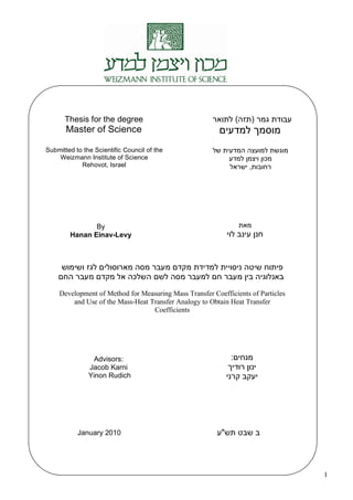
- 38. (a) (c) bypass S bypass S TD N R M S bypass S TD N Rbypass M Minimum 0.805 0.88 260 1.6 - - 200 2.2 Average 0.81 0.92 310 2.1 - - 430 2.8 Maximum 0.815 0.94 360 2.7 - - 660 3.6 Figure 18: Effect of residence time. 300 nm PSL sphere (a) 25-30 nm BaP coating, TD flow rate sweep 80-260 cc/min at 85 o (b) 20 nm BaP coating, size selected by second DMA, TD flow sweep 380-1240 cc/min at 85 o (a) (b) (c) bypass bypass S bypass S TD N R M S bypass S TD N R M S bypass S TD N Rbypass M Minimum 0.85 0.91 200 2.5 0.77 0.8 75 3.44 0.84 0.87 190 2.1 Average 0.87 0.94 380 2.85 0.81 0.84 500 4.3 0.85 0.89 320 2.4 Maximum 0.88 0.97 570 3.1 0.85 0.88 1550 7.07 0.86 0.91 440 2.7 Figure 19: Effect of residence time. 400 nm PSL sphere (a) 22-30 nm BaP coating, TD flow rate sweep 300-1100 cc/min at 95 o (b) 25-30 nm BaP coating, TD flow rate sweep 380-500 cc/min at 90 o (upper 3 points), TD flow rate sweep 115-500 cc/min at 85 o (rest of points) (c) 22-30 nm BaP coating, TD flow rate sweep 290-470 cc/min at 85 o . Associated table displays minimum, maximum and average values for the Jayne shape factor (see page 33) of the coated particles S bypass , evaporated particles S TD , number concentration N[#/ cc] and calibration ratio Rbypass M 37
- 39. 4 Discussion 4.1 Derivation of the Sherwood number Figure 20: Sherwood number vs. particle diameter for experiments shown in figures 17-19 The Sherwood number (Sh) was derived for different nominal PSL sphere diameters according to Equation (25), and is compared to the theoretical diffusive mass transfer case in the transition regime, using Eq (12) (Davies (1978) from Hinds (1999) p. 288) 2" + D ShKn = 2·! (Kn) = 2· D + 5.33(" 2 D) + 3.42 " Theoretically, for a spherical particle, in the continuum regime, where no convective mass transfer occurs, Sh should equal 2. This is corrected for the transition regime using Eq (12), which leads to lower Sh. Figure 20 presents the derived Sherwood number for different PSL diameters and driving force. The dotted line represents the calculated ShKn numbers for these conditions. It can be seen that most of the measurements fall close to this line, within the measurement errors. The free kT mean path ! was calculated according to ! = [m] where p = 101325[Pa] and T is the "d p 2 2 N2 average of the flat part of the oven, as seen in the bottom of Figure 11. The mass loss calculation, based on AMS and SMPS, or only on SMPS, are shown in section 3.1.5.3 . 38