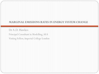
3. Residential Sector Heating
1600
Demand Response
1400 District Heating
Solar Thermal
1200
Demand Served (PJ/year)
Heat Pump
1000
Conservation
800 Wood Boiler
Solid Fuel Boiler
600
Pellet Boiler
400
Oil Boiler
200
Gas Boiler
0 Coal Boiler
2000 2010 2020 2030 2040 2050
Direct Electric
4. CO2 Reduction Performance
Which demand-side technology?
How much CO2 will it save?
Which “baseline” technology will it displace?
Where there is an interaction with the electricity system, how
much CO2 will be saved/produced for every kWh saved/used?
What about interactions with other parts of the energy system –
primary resource choice, sectoral focus of emissions reduction,
etc?
5. The usual method
Choose a baseline system
E.g. For heating in the UK; the combustion of natural gas in a condensing boiler
Figure out how much of each “energy carrier” the alternative
system saves/produces (relative to the consumption/production
of the baseline).
E.g. A CHP system may consume an additional 3000kWh of gas/year, and
produce an additional 2500kWh of electricity
Multiply change in consumption for each energy carrier by the
respective standard emissions rates; ~0.19kgCO2/kWh for gas,
and 0.43kgCO2/kWh for electricity in the UK
E.g. Change in CO2 = 0.19*3000 – 0.43*2500 = -1075kg CO2
6. An alternative method - marginal CO2 rates
The CO2 actually saved due to a change in electricity demand is
related to which power stations actually respond to that change.
7. The observed response of generators in GB
ELEXON publishes pre-gate closure dispatch data for every “BM
unit” in the GB system
We know which generators these are, and their efficiency, so we
can calculate the CO2 production rate change associated with a
change in output
We can do this for every generator, so we can find the aggregate
change in CO2 produced in any ½ hour period, along with the
change in aggregate system load
We can create a scatter plot of these
We can create a linear fit (through zero)
The slope of the linear fit is an estimate of the marginal emissions
rate for the system
8. GB Electricity Marginal Emissions
2002 to 2009 inclusive
Change in System CO2 Rate (ktCO2/h)
Linear Fit: y = 0.69 x
Change in System Load (GWh/h)
Source: Hawkes, A.D. (2010) Estimating Marginal Emissions Rates in National Electricity Systems. Energy Policy 38(10) 5977-5987.
doi:10.1016/j.enpol.2010.05.053
9. Change in System CO2 Rate (ktCO2/h)
y = 0.69 x
Change in System Load (GWh/h)
Marginal Emissions Factor (kgCO2/kWh)
Stats of the MEF
GB System Load (GW)
Probability of System Load
Number of Observations
Change in System Load (GWh/h)
10. Change over time
Decommissioning and commissioning of power stations.
We know which “BM Units” will be decommissioned out to
~2020. National Grid also projects the types of new
generators over the same period.
We can replace the old with the new, and repeat the marginal
emissions calculation.
Resulting in...
Time Period Marginal Emissions Rate
(kgCO2/kWh)
2002-2009 0.69 kgCO2/kWh
2016 0.6 kgCO2/kWh
2020-2025 0.51 kgCO2/kWh
11. What does this mean?
The actual marginal emissions rate from 2002-2009 was 60%
higher than the figure typically used in policy analysis.
12. But...
What about changes elsewhere in the energy system, and
over a much longer timeframe?
=> Analysis using the UK MARKAL Model
MARKAL (Market Allocation) chooses the least cost pathway for
energy system change over a 50 year time horizon. It is an
optimisation model, with objective function of discounted
system cost, user-defined constraints, and thousands of decision
variables.
13. MARKAL Analysis Method
Constrain the introduction of micro-CHP and heat pumps
into the energy system
Zero to 10,000,000 installations, in 1,000,000 increments
Run MARKAL, record change in total system CO2 emissions
over the entire time horizon
Calculate the abatement associated with the introduction of
each system (i.e. CO2 reduction per system per year)
Allow all other aspects of the energy system to respond
dynamically to the “forced” introduction of the intervention
15. Conclusion
From 2002-2009, the marginal CO2 intensity of grid
electricity in Great Britain was 0.69 kgCO2/kWh.
But the long term CO2 reduction brought about by a class of
interventions is more reliant on long term system changes
than short term....but MARKAL is a crude tool for such
analyses, and more research would be required to make firm
conclusions.
A stronger link between demand-side modelling and system
modelling is required to assess this situation more accurately.
16. Key Challenge: which margin?
A hypothetical situation:
1. We adopt a new technology (e.g. an electric car)
2. This technology causes an increase in peak system load (i.e. it
has negative capacity credit).
3. THEREFORE => the electric car is responsible for all the
emissions increase/decrease associated with that power
station. This is the BUILD MARGIN PERSPECTIVE.
4. BUT, when we actually charge the car, it is not the new
power station that responds to this demand.
5. THEREFORE, the operational marginal emissions rate is
appropriate. This is the OPERATING MARGIN
PERSPECTIVE.