Data Mining Un-Compressed Images from cloud with Clustering Compression technique using Lempel-Ziv-Welch

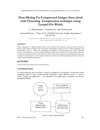
International Journal of Artificial Intelligence & Applications (IJAIA), Vol. 4, No. 4, July 2013
DOI : 10.5121/ijaia.2013.4413 145
Data Mining Un-Compressed Images from cloud
with Clustering Compression technique using
Lempel-Ziv-Welch
1
C. Parthasarathy 2
K.Srinivasan and 3
R.Saravanan
Assistant Professor, 1,2,3
Dept. of I.T, SCSVMV University, Enathur, Kanchipuram,
Pin–631 561
1
sarathy286089@rediffmail.com 2
kadamsrini21@gmail.com
3
saravanan_kpm1983@yahoo.co.in
ABSTRACT
Cloud computing is a highly discussed topic in the technical and economic world, and many of the big
players of the software industry have entered the development of cloud services. Several companies’ and
organizations wants to explore the possibilities and benefits of incorporating such cloud computing
services in their business, as well as the possibilities to offer own cloud services. We are going to mine the
un-compressed image from the cloud and use k-means clustering grouping the uncompressed image and
compress it with Lempel-ziv-welch coding technique so that the un-compressed images becomes error-free
compression and spatial redundancies.
KEYWORDS
Cloud, Compression, Image processing, Clustering
1. INTRODUCTION
In cloud computing, the word cloud is used as a metaphor for “the Internet” so the phrase cloud
computing means "a type of Internet-based computing," where different services -- such as
servers, storage and applications -- are delivered to an organization's computers and devices
through the Internet.
Figure 1. Cloud Computing Model
Cloud
service
(queue)
Cloud
Infrastructure
(Billing VMs)
Cloud Platform
(eg. web front end)
Cloud storage
(Eg. Data base)

146
Clustering can be considered the most important unsupervised learning technique; so, as every
other problem of this kind, it deals with finding a structure in a collection of unlabeled data.
Clustering is “the process of organizing objects into groups whose members are similar in some
way”. A cluster is therefore a collection of objects which are “similar” between them and are
“dissimilar” to the objects belonging to other clusters. The typical requirements of clustering in
data mining are 1. Scalability 2. Ability to deal with different types of attributes 3. Discovery of
clusters with arbitrary shape 4. Minimal requirements for domain knowledge to determine input
parameters 5. Ability to deal with noisy data 6. Incremental clustering and insensitivity to the
order of input records. 7. High dimensionality. Clustering is also called data segmentation
because clustering partitions large data sets into groups according to their similarity.
2. K-MEANS METHOD
In this cloud we are going to cluster the un-compressed Image by centroid based technique: The
K-means algorithm takes input parameter and partitions a set of n-objects into k clusters so that
the resulting intra-cluster similarity is high but the inter-cluster similarity is low. K-Means
algorithm proceeds as it randomly selects k of the objects, an object is assigned to the cluster it is
the most similar, based on the distance between the object and the cluster mean. It Computes the
new mean for each cluster it iterates until the criterion function converges.
The square-error criterion
k
E = ∑ ∑ | p-mi| 2 where E is the sum of the square error for all
objects in
i=1 pɛCi
the data set; p is the point in space representing a given object and mi is the mean of cluster Ci
Algorithm: The k-means algorithm for partitioning, where each cluster’s center is represented by
the mean value of the objects in the cluster.
Input :
k: the number of clusters
D: a data set containing n objects
Method:
(1) arbitrarily choose k objects from D as the initial cluster centers Repeat Assign each
object to the cluster to which the object is the most similar Based on the mean value of
the objects in the cluster; Update the cluster means, i.e., calculate the mean value of the
object for Each cluster; Until no change.
.
Figure 2. shows the mean m1,m2 is far away from the final boundary

147
Figure 3. shows how the means m1 and m2 move closer to the final boundary
Figure 4. shows different types of clusters
After the algorithm finishes, it produces these outputs:
• A label for each data point
• The center for each label
A label can be considered as “assigning a group”. For example, in the above image you can see
four “labels”. Each label is displayed with a different colour. All yellow points could have the
label 0, orange could have label 1, etc.

148
Figure 5. Grouping different set of uncompressed images
Step 0: Get the dataset
As an example, We will be using the data points on the left. We’ll assume K=5. And it’s
apparent that this dataset has 5 clusters: three spaced out and two almost merging.
Step 1: Assign random centers
The first step is to randomly assign K centers. We have marked them as red points in the image.
Note how they are all concentrated in the two “almost merging” clusters. These centers are just an
initial guess. The algorithm will iteratively correct itself. Finally, these centers will coincide with
the actual center of each cluster.
Step 2: “Own” datapoints
Each datapoint checks which center it is closest to. So, it “belongs” to that particular center. Thus,
all centers “own” some number of points.
Step 3: Shift the centers
Each center uses the points it “owns” to calculate a new center. Then, it shifts itself to that center.
If the centers actually shifted, we again go to Step 3. If not, then the centers are the final result.
We proceed to the next step
Now that the centers do not move, you can use the centers.
3. SCOPE OF THE RESEARCH
We know about the term compression ratio. This means as:
Compression Ratio , Cr= ((Data size of original message)/ (Data size of Encoded message))
Now-a-days, compression ratio is a great factor in transmission of data. By this research we can
have a better solution about how to make compression ratio higher, because data transmission
mostly depends on compression ratio. Images transmitted over the world wide web here data
compression is important. Suppose we need to download a digitized color photograph over a
computer's 33.6 kbps modem. If the image is not compressed (a TIFF file, for example), it will
contain about 600 kbytes of data. If it has been compressed using a LSW CODING technique
(such as used in the GIF format),it will be about one-half this size, or 300 kbytes. If LSW
CODING TECHNIQUE has been used (a JPEG file), it will be about 50 kbytes. The point is, the
download times for these three equivalent files are 142 seconds, 71 seconds, and 12 seconds,
respectively. Digitized photographs, while GIF is used with drawn images, such as company
logos that have large areas of a single color.
Disadvantage of Lossless Compression
Lossless compression, refers to the process of encoding data more efficiently so that it occupies
fewer bits or bytes but in such a way that the original data can be reconstructed, bit-for-bit, when

149
the data is decompressed. The advantage of lossless encoding techniques is that they produce an
exact duplicate of the original data but they also have some disadvantages when compared to
Lossy encoding techniques.
4. COMPRESSION RATIO
Lossless encoding techniques cannot achieve high levels of compression. Few lossless encoding
techniques can achieve a compression ratio higher than 8:1 which compares unfavorably with so-
called lossy encoding techniques. Lossy encoding techniques -- which achieve compression by
discarding some of the original data -- can achieve compression ratios of 10:1 for audio and 300:1
for video with little or no perceptible loss of quality. According to the New Biggin Photography
Group a 1,943 by 1,702 pixel 24-bit RGB color image with an original size of 9.9 megabytes can
only be reduced to 6.5 megabytes using the lossless PNG format but can be reduced to just 1
megabyte using the lossy JPEG format.
5. TRANSFER TIME
Any application that involves storing or distributing digital images, or both, presupposes that
these operations can be completed in a reasonable length of time. The time needed to transfer a
digital image depends on the size of the compressed image and as the compression ratios that can
be achieved by lossless encoding techniques are far lower than lossy encoding techniques,
lossless encoding techniques are unsuitable for these applications.
5.1. Lempel-Ziv-Welch (Lzw) Coding Technique
LZW compression is named after its developers, A. Lempel and J. Ziv, with later modifications
by Terry A. Welch. It is the foremost technique for general purpose data compression due to its
simplicity and versatility. Typically, you can expect LZW to compress text, executable code, and
similar data files to about one-half their original size. LZW also performs well when presented
with extremely redundant data files, such as tabulated numbers, computer source code, and
acquired signals. Compression ratios of 5:1 are common for these cases.
LZW compression uses a code table, as illustrated in Fig. 6. A common choice is to provide 4096
entries in the table. In this case, the LZW encoded data consists entirely of 12 bit codes, each
referring to one of the entries in the code table. Un compression is achieved by taking each code
from the compressed file, and translating it through the code table to find what character or
characters it represents. Codes 0-255 in the code table are always assigned to represent single
bytes from the input file. For example, if only these first 256 codes were used, each byte in the
original file would be converted into 12 bits in the LZW encoded file, resulting in a 50% larger
file size. During un compression, each 12 bit code would be translated via the code table back
into the single bytes. Of course, this wouldn't be a useful situation.
6. ADVANTAGE OF LZW COMPRESSION
The LZW compression can compress executable code, text, and similar data files to almost one-
half of their original size. It usually uses single codes to replace strings of characters, thereby
compressing the data. LZW also gives a good performance when extremely redundant data files
are presented to it like computer source code, tabulated numbers and acquired signals. The
common compression ratio for these cases is almost in the range of 5:1.

150
Figure 6 – Flow chart for LZW coding compression
Many methods of LZW coding compression have been developed; however, a family of
techniques called transform compression has proven the most valuable. The best example of
transform compression is embodied in the popular JPEG standard of image encoding. JPEG is
named after its origin, the Joint Photographers Experts Group. LZW compression is different
from other common compression algorithms (e.g. Huffman encoding) in that it does not require
an initial processing of the data file to determine the codes to be used. Instead, the code table is
generated “on the fly” at the same time that the file is compressed. The algorithm operates so that
at each basic step, either the code for a sequence of values already exists in the table, or the code
for a new sequence is generated and inserted into the table. Another interesting characteristic of
LZW compression is that it is not necessary to send a full code table along with the compressed
file. Only a table of the individual colors that exist in the image is needed. Then codes for
sequences of colors are generated during the decompression process such that the codes are
always available in the table when they are needed.
START
INPUT FIRST BYTE
STORE IN STRING
INPUT NEXT BYTE
STORE IN CHAR
IS STRING-
CHAR IN
TABLE
OUTPUT THE CODE
FOR STRING
STRING = STRING
+CHAR
STRING = CHAR
ADD ENTRY TABLE FOR
STRING + CHAR
MORE BYTES
TO INPUT ?
OUTPUT THE CODE
FOR STRING
STOP

151
The first step in LZW is initialization of the code table to include all the colors in the image file.
For an 8-bit image, this would be up to 256 colors. If all colors were used, the codes would be
the values from 0 through 255, each code requiring eight bits. The algorithm proceeds by
processing the pixels in the image file from left to right and top to bottom of the image. The basic
idea of the algorithm is that strings of colors are put into the code table as they are encountered.
Grouping strings of colors together into a single code results in compression.
The basic algorithm for LZW compression is given below. In the pseudocode that follows,
pixelString is a sequence of pixel values. pixel = next pixel value means “read the next pixel out
of the image file.” pixelString + pixel means “take the current pixelString value and concatenate
pixel onto the end of it.”
algorithm LZW
/*Input: A bitmap image
Output: A table of the individual colors in the image and a compressed version of the file
Note that + is concatenation*/
{
initialize table to contain the individual colors in bitmap
pixelString = first pixel value
while there are still pixels to process {
pixel = next pixel value
stringSoFar = pixelString + pixel
if stringSoFar is in the table then
pixelString = stringSoFar
else {
output the code for pixelString
add stringSoFar to the table
pixelString = pixel
}
}
output the code for pixelString
}
Consider an simplified problem a string BABAABAAA use the LZW Algorithm to compress the string.[
TABLE-1 EXAMPLE WORK FOR COMPRESSION

152
A simplified examplealgorithm LZW_decompress
/*Input: Compressed bitmap image and table of individual colors in image
Output: Decompressed image*/
{
/*Initialize table*/
stringSoFar = NULL
while there are still codes to process in the code string {
code = next code in the code string
colors = the colors corresponding to code in the table
if colors == NULL /*Case where code is not in the table*/
/*stringSoFar0 is the first color in stringSoFar*/
colors = stringSoFar + stringSoFar0
output colors
if stringSoFar != NULL
put stringSoFar + colors0 in the table
stringSoFar = colors
}
}
Basic LZW Decompression Algorithm
A simplified example for the string BABAABAAA the compressed code words are
<66><65><256><257><258><259><260> using the code word we are going to de-compress the
information
TABLE -2 EXAMPLE WORK FOR DE-COMPRESSION
Encoder output string String table code-word String
B
A 256 BA
BA 257 AB
AB 258 BAA
A 259 ABA
AA 260 AA

153
Figure 7. JPEG IMAGE DIVISION
JPEG image division. JPEG transform compression starts by breaking the image into 8×8 groups,
each containing 64 pixels. Three of these 8×8 groups are enlarged in this figure, showing the
valuesof the individual pixels, a single byte value between 0 and 255.
A. Original image

154
B. With 10:1 Compression
C. With 45:1 Compression
Figure 8 Example of JPEG distortion. Figure(a) shows the original image, while (b) and (c) shows
restored images using compression ratios of 10:1 and 45:1, respectively. The high compression
ratio used in (c) results in each 8X8 pixel group being represented by less than 12 bits.
Figure 9. A plot of the intensity data of line 266 of the original (uncompressed) image

155
Figure 10. A plot of the intensity data of line 266 of the 1.0 bpp NSI compressed image.
7. CONCLUSION
Image compression is a topic of much importance and employed in many applications. Methods
of Image compression have been studied for almost four decades. An enhanced scaling algorithm
was devised. This algorithm utilized the proximity of the sample points chosen to each other to
detect edges This paper has provided an overview of Image compression methods of general
utility. The algorithms have been evaluated in terms of the amount of compression they provide,
algorithm efficiency, and susceptibility to error. While algorithm efficiency and susceptibility to
error are relatively independent of the characteristics of the source ensemble, the amount of
compression achieved depends upon the characteristics of the source to a great extent.
REFERENCES
[1] “Digital Image Processing” Second paper Edition-(2006) ,Rafael C. Gonzalez and Richard E. Woods.
Pages: 411, 440-442, 459.
[2] “Lecture on Data Compression” , Patrick Karlsson Patrick. karlsson@cb.uu.se
[3] “Error-Resilient LZW Data Compression” , YonghuiWu Stefano Lonardi WojciechSzpankowski,
Proceedings of the Data Compression Conference IEEE(DCC’06) 0-7695-2545-8 /06 (2006)
[4] "LZW Data Compression" Mark Nelson's from the October, 1989 issue of Dr. Dobb's Journal.
[5] “A fast binary template matching algorithm for document image data compression in Pattern
Recognition”, Holt, M.J. (1988) J. Kittler (ed.) (Proc. Int. Conf.,Cambridge). Springer Verlag, Berlin.
[6] “Compression of black-white images with arithmetic coding,” Langdon, G.G. and Rissanen, J.
(1981)June IEEE Trans Communications COM-29(6): 858–867.
[7] “Two level context based compression of binary images”,in Proc. DCC’91, J.A. Storer and J.H. Reif
(eds.), Moffat, A. IEEE Computer Society Press, Los Alamitos (1991) pp. 382-391.
[8] “Combined symbol matching facsimile data compression system”, Pratt, W.K., Capitant, P.J., Chen,
W.H.,Hamilton, E.R. and Wallis, R.H. (1980) July Proc IEEE 68(7): 786-796;.
[9] “Textual Image Compression” in Proc.DCC’92, J.A. Storer and M. Cohn (eds.),Witten, I.H., Bell,
Harrison, James and Moffat, A. IEEE Computer Society Press, Los Alamitos, CA. (1992) pp. 42-51.
[10] “A universal algorithm for sequential data compression”, ZIV, J. AND LEMPEL, A.(197I)IEEE
Trans. Inform. Theory 23, 3, 337–343.
[11] “Text Compression English word” T. C. Bell, J. G. Cleary, and I. H. Witten,C1iffs:N. J. Prentice-
Hall, 1990.
[12] “The LEMPEL-ZIV-WEL (LZW) Data Compression Algorithm for Packet Radio”, Kinsner and R H.
Greenfield –IEEE
[13] “Enhanced LZW (Lempel-Ziv-Welch) Algorithm with Binary Search to Reduce Time Complexity
for Dictionary Creation in Encoding and Decoding”, published Proceedings of international
conference(ICICIC 2012) NISHAD PM and Dr. N. NALAYINI -PSG tech 5- January 2012.
[14] "PPM performance with BWT Complexity: A fast and effective data compression algorithm", M.
Effros,Proceedings of the IEEE, 88(11), 1703-1712, (2000).
[15] "Compression of two-dimensional data", A. Lempel and J. Ziv, IEEE Transactions on Information
Theory, 32(1), 2-8, (1986).

Data Mining Un-Compressed Images from cloud with Clustering Compression technique using Lempel-Ziv-Welch

Recommandé

Recommandé

Contenu connexe

Tendances

Tendances (19)

Similaire à Data Mining Un-Compressed Images from cloud with Clustering Compression technique using Lempel-Ziv-Welch

Similaire à Data Mining Un-Compressed Images from cloud with Clustering Compression technique using Lempel-Ziv-Welch (20)

Dernier

Dernier (20)

Data Mining Un-Compressed Images from cloud with Clustering Compression technique using Lempel-Ziv-Welch