SlideShare une entreprise Scribd logo
1  sur  44
Télécharger pour lire hors ligne
15 THERMODYNAMICS
Figure 15.1 A steam engine uses heat transfer to do work. Tourists regularly ride this narrow-gauge steam engine train near the San Juan Skyway in Durango, Colorado, part
of the National Scenic Byways Program. (credit: Dennis Adams)
Learning Objectives
15.1. The First Law of Thermodynamics
• Define the first law of thermodynamics.
• Describe how conservation of energy relates to the first law of thermodynamics.
• Identify instances of the first law of thermodynamics working in everyday situations, including biological metabolism.
• Calculate changes in the internal energy of a system, after accounting for heat transfer and work done.
15.2. The First Law of Thermodynamics and Some Simple Processes
• Describe the processes of a simple heat engine.
• Explain the differences among the simple thermodynamic processes—isobaric, isochoric, isothermal, and adiabatic.
• Calculate total work done in a cyclical thermodynamic process.
15.3. Introduction to the Second Law of Thermodynamics: Heat Engines and Their Efficiency
• State the expressions of the second law of thermodynamics.
• Calculate the efficiency and carbon dioxide emission of a coal-fired electricity plant, using second law characteristics.
• Describe and define the Otto cycle.
15.4. Carnot’s Perfect Heat Engine: The Second Law of Thermodynamics Restated
• Identify a Carnot cycle.
• Calculate maximum theoretical efficiency of a nuclear reactor.
• Explain how dissipative processes affect the ideal Carnot engine.
15.5. Applications of Thermodynamics: Heat Pumps and Refrigerators
• Describe the use of heat engines in heat pumps and refrigerators.
• Demonstrate how a heat pump works to warm an interior space.
• Explain the differences between heat pumps and refrigerators.
• Calculate a heat pump’s coefficient of performance.
15.6. Entropy and the Second Law of Thermodynamics: Disorder and the Unavailability of Energy
• Define entropy.
• Calculate the increase of entropy in a system with reversible and irreversible processes.
• Explain the expected fate of the universe in entropic terms.
• Calculate the increasing disorder of a system.
15.7. Statistical Interpretation of Entropy and the Second Law of Thermodynamics: The Underlying Explanation
• Identify probabilities in entropy.
• Analyze statistical probabilities in entropic systems.
CHAPTER 15 | THERMODYNAMICS 507
Introduction to Thermodynamics
Heat transfer is energy in transit, and it can be used to do work. It can also be converted to any other form of energy. A car engine, for example,
burns fuel for heat transfer into a gas. Work is done by the gas as it exerts a force through a distance, converting its energy into a variety of other
forms—into the car’s kinetic or gravitational potential energy; into electrical energy to run the spark plugs, radio, and lights; and back into stored
energy in the car’s battery. But most of the heat transfer produced from burning fuel in the engine does not do work on the gas. Rather, the energy is
released into the environment, implying that the engine is quite inefficient.
It is often said that modern gasoline engines cannot be made to be significantly more efficient. We hear the same about heat transfer to electrical
energy in large power stations, whether they are coal, oil, natural gas, or nuclear powered. Why is that the case? Is the inefficiency caused by design
problems that could be solved with better engineering and superior materials? Is it part of some money-making conspiracy by those who sell energy?
Actually, the truth is more interesting, and reveals much about the nature of heat transfer.
Basic physical laws govern how heat transfer for doing work takes place and place insurmountable limits onto its efficiency. This chapter will explore
these laws as well as many applications and concepts associated with them. These topics are part of thermodynamics—the study of heat transfer
and its relationship to doing work.
15.1 The First Law of Thermodynamics
Figure 15.2 This boiling tea kettle represents energy in motion. The water in the kettle is turning to water vapor because heat is being transferred from the stove to the kettle.
As the entire system gets hotter, work is done—from the evaporation of the water to the whistling of the kettle. (credit: Gina Hamilton)
If we are interested in how heat transfer is converted into doing work, then the conservation of energy principle is important. The first law of
thermodynamics applies the conservation of energy principle to systems where heat transfer and doing work are the methods of transferring energy
into and out of the system. The first law of thermodynamics states that the change in internal energy of a system equals the net heat transfer into
the system minus the net work done by the system. In equation form, the first law of thermodynamics is
(15.1)ΔU = Q − W.
Here ΔU is the change in internal energy U of the system. Q is the net heat transferred into the system—that is, Q is the sum of all heat
transfer into and out of the system. W is the net work done by the system—that is, W is the sum of all work done on or by the system. We use the
following sign conventions: if Q is positive, then there is a net heat transfer into the system; if W is positive, then there is net work done by the
system. So positive Q adds energy to the system and positive W takes energy from the system. Thus ΔU = Q − W . Note also that if more heat
transfer into the system occurs than work done, the difference is stored as internal energy. Heat engines are a good example of this—heat transfer
into them takes place so that they can do work. (See Figure 15.3.) We will now examine Q , W , and ΔU further.
508 CHAPTER 15 | THERMODYNAMICS
This content is available for free at http://cnx.org/content/col11406/1.7
Figure 15.3 The first law of thermodynamics is the conservation-of-energy principle stated for a system where heat and work are the methods of transferring energy for a
system in thermal equilibrium. Q represents the net heat transfer—it is the sum of all heat transfers into and out of the system. Q is positive for net heat transfer into the
system. W is the total work done on and by the system. W is positive when more work is done by the system than on it. The change in the internal energy of the system,
ΔU , is related to heat and work by the first law of thermodynamics, ΔU = Q − W .
Making Connections: Law of Thermodynamics and Law of Conservation of Energy
The first law of thermodynamics is actually the law of conservation of energy stated in a form most useful in thermodynamics. The first law gives
the relationship between heat transfer, work done, and the change in internal energy of a system.
Heat Q and Work W
Heat transfer ( Q ) and doing work ( W ) are the two everyday means of bringing energy into or taking energy out of a system. The processes are
quite different. Heat transfer, a less organized process, is driven by temperature differences. Work, a quite organized process, involves a
macroscopic force exerted through a distance. Nevertheless, heat and work can produce identical results.For example, both can cause a temperature
increase. Heat transfer into a system, such as when the Sun warms the air in a bicycle tire, can increase its temperature, and so can work done on
the system, as when the bicyclist pumps air into the tire. Once the temperature increase has occurred, it is impossible to tell whether it was caused by
heat transfer or by doing work. This uncertainty is an important point. Heat transfer and work are both energy in transit—neither is stored as such in a
system. However, both can change the internal energy U of a system. Internal energy is a form of energy completely different from either heat or
work.
Internal Energy U
We can think about the internal energy of a system in two different but consistent ways. The first is the atomic and molecular view, which examines
the system on the atomic and molecular scale. The internal energy U of a system is the sum of the kinetic and potential energies of its atoms and
molecules. Recall that kinetic plus potential energy is called mechanical energy. Thus internal energy is the sum of atomic and molecular mechanical
energy. Because it is impossible to keep track of all individual atoms and molecules, we must deal with averages and distributions. A second way to
view the internal energy of a system is in terms of its macroscopic characteristics, which are very similar to atomic and molecular average values.
Macroscopically, we define the change in internal energy ΔU to be that given by the first law of thermodynamics:
(15.2)ΔU = Q − W.
Many detailed experiments have verified that ΔU = Q − W , where ΔU is the change in total kinetic and potential energy of all atoms and
molecules in a system. It has also been determined experimentally that the internal energy U of a system depends only on the state of the system
and not how it reached that state. More specifically, U is found to be a function of a few macroscopic quantities (pressure, volume, and temperature,
for example), independent of past history such as whether there has been heat transfer or work done. This independence means that if we know the
state of a system, we can calculate changes in its internal energy U from a few macroscopic variables.
Making Connections: Macroscopic and Microscopic
In thermodynamics, we often use the macroscopic picture when making calculations of how a system behaves, while the atomic and molecular
picture gives underlying explanations in terms of averages and distributions. We shall see this again in later sections of this chapter. For
example, in the topic of entropy, calculations will be made using the atomic and molecular view.
To get a better idea of how to think about the internal energy of a system, let us examine a system going from State 1 to State 2. The system has
internal energy U1 in State 1, and it has internal energy U2 in State 2, no matter how it got to either state. So the change in internal energy
ΔU = U2 − U1 is independent of what caused the change. In other words, ΔU is independent of path. By path, we mean the method of getting
from the starting point to the ending point. Why is this independence important? Note that ΔU = Q − W . Both Q and W depend on path, but
ΔU does not. This path independence means that internal energy U is easier to consider than either heat transfer or work done.
CHAPTER 15 | THERMODYNAMICS 509
Example 15.1 Calculating Change in Internal Energy: The Same Change in U is Produced by Two Different
Processes
(a) Suppose there is heat transfer of 40.00 J to a system, while the system does 10.00 J of work. Later, there is heat transfer of 25.00 J out of the
system while 4.00 J of work is done on the system. What is the net change in internal energy of the system?
(b) What is the change in internal energy of a system when a total of 150.00 J of heat transfer occurs out of (from) the system and 159.00 J of
work is done on the system? (See Figure 15.4).
Strategy
In part (a), we must first find the net heat transfer and net work done from the given information. Then the first law of thermodynamics
⎛
⎝ΔU = Q − W⎞
⎠ can be used to find the change in internal energy. In part (b), the net heat transfer and work done are given, so the equation
can be used directly.
Solution for (a)
The net heat transfer is the heat transfer into the system minus the heat transfer out of the system, or
(15.3)Q = 40.00 J − 25.00 J = 15.00 J.
Similarly, the total work is the work done by the system minus the work done on the system, or
(15.4)W = 10.00 J − 4.00 J = 6.00 J.
Thus the change in internal energy is given by the first law of thermodynamics:
(15.5)ΔU = Q − W = 15.00 J − 6.00 J = 9.00 J.
We can also find the change in internal energy for each of the two steps. First, consider 40.00 J of heat transfer in and 10.00 J of work out, or
(15.6)ΔU1 = Q1 − W1 = 40.00 J − 10.00 J = 30.00 J.
Now consider 25.00 J of heat transfer out and 4.00 J of work in, or
(15.7)ΔU2 = Q2 − W2= - 25.00 J − ( − 4.00 J ) = –21.00 J.
The total change is the sum of these two steps, or
(15.8)ΔU = ΔU1 + ΔU2 = 30.00 J + (−21.00 J ) = 9.00 J.
Discussion on (a)
No matter whether you look at the overall process or break it into steps, the change in internal energy is the same.
Solution for (b)
Here the net heat transfer and total work are given directly to be Q = – 150.00 J and W = – 159.00 J , so that
(15.9)ΔU = Q – W = – 150.00 J – ( − 159.00 J) = 9.00 J.
Discussion on (b)
A very different process in part (b) produces the same 9.00-J change in internal energy as in part (a). Note that the change in the system in both
parts is related to ΔU and not to the individual Q s or W s involved. The system ends up in the same state in both (a) and (b). Parts (a) and
(b) present two different paths for the system to follow between the same starting and ending points, and the change in internal energy for each
is the same—it is independent of path.
510 CHAPTER 15 | THERMODYNAMICS
This content is available for free at http://cnx.org/content/col11406/1.7
Figure 15.4 Two different processes produce the same change in a system. (a) A total of 15.00 J of heat transfer occurs into the system, while work takes out a total of 6.00 J.
The change in internal energy is ΔU = Q − W = 9.00 J . (b) Heat transfer removes 150.00 J from the system while work puts 159.00 J into it, producing an increase of
9.00 J in internal energy. If the system starts out in the same state in (a) and (b), it will end up in the same final state in either case—its final state is related to internal energy,
not how that energy was acquired.
Human Metabolism and the First Law of Thermodynamics
Human metabolism is the conversion of food into heat transfer, work, and stored fat. Metabolism is an interesting example of the first law of
thermodynamics in action. We now take another look at these topics via the first law of thermodynamics. Considering the body as the system of
interest, we can use the first law to examine heat transfer, doing work, and internal energy in activities ranging from sleep to heavy exercise. What
are some of the major characteristics of heat transfer, doing work, and energy in the body? For one, body temperature is normally kept constant by
heat transfer to the surroundings. This means Q is negative. Another fact is that the body usually does work on the outside world. This means W is
positive. In such situations, then, the body loses internal energy, since ΔU = Q − W is negative.
Now consider the effects of eating. Eating increases the internal energy of the body by adding chemical potential energy (this is an unromantic view
of a good steak). The body metabolizes all the food we consume. Basically, metabolism is an oxidation process in which the chemical potential
energy of food is released. This implies that food input is in the form of work. Food energy is reported in a special unit, known as the Calorie. This
energy is measured by burning food in a calorimeter, which is how the units are determined.
In chemistry and biochemistry, one calorie (spelled with a lowercase c) is defined as the energy (or heat transfer) required to raise the temperature of
one gram of pure water by one degree Celsius. Nutritionists and weight-watchers tend to use the dietary calorie, which is frequently called a Calorie
(spelled with a capital C). One food Calorie is the energy needed to raise the temperature of one kilogram of water by one degree Celsius. This
means that one dietary Calorie is equal to one kilocalorie for the chemist, and one must be careful to avoid confusion between the two.
Again, consider the internal energy the body has lost. There are three places this internal energy can go—to heat transfer, to doing work, and to
stored fat (a tiny fraction also goes to cell repair and growth). Heat transfer and doing work take internal energy out of the body, and food puts it back.
If you eat just the right amount of food, then your average internal energy remains constant. Whatever you lose to heat transfer and doing work is
replaced by food, so that, in the long run, ΔU = 0 . If you overeat repeatedly, then ΔU is always positive, and your body stores this extra internal
energy as fat. The reverse is true if you eat too little. If ΔU is negative for a few days, then the body metabolizes its own fat to maintain body
temperature and do work that takes energy from the body. This process is how dieting produces weight loss.
Life is not always this simple, as any dieter knows. The body stores fat or metabolizes it only if energy intake changes for a period of several days.
Once you have been on a major diet, the next one is less successful because your body alters the way it responds to low energy intake. Your basal
metabolic rate (BMR) is the rate at which food is converted into heat transfer and work done while the body is at complete rest. The body adjusts its
basal metabolic rate to partially compensate for over-eating or under-eating. The body will decrease the metabolic rate rather than eliminate its own
fat to replace lost food intake. You will chill more easily and feel less energetic as a result of the lower metabolic rate, and you will not lose weight as
fast as before. Exercise helps to lose weight, because it produces both heat transfer from your body and work, and raises your metabolic rate even
when you are at rest. Weight loss is also aided by the quite low efficiency of the body in converting internal energy to work, so that the loss of internal
energy resulting from doing work is much greater than the work done.It should be noted, however, that living systems are not in thermalequilibrium.
The body provides us with an excellent indication that many thermodynamic processes are irreversible. An irreversible process can go in one
direction but not the reverse, under a given set of conditions. For example, although body fat can be converted to do work and produce heat transfer,
CHAPTER 15 | THERMODYNAMICS 511
work done on the body and heat transfer into it cannot be converted to body fat. Otherwise, we could skip lunch by sunning ourselves or by walking
down stairs. Another example of an irreversible thermodynamic process is photosynthesis. This process is the intake of one form of
energy—light—by plants and its conversion to chemical potential energy. Both applications of the first law of thermodynamics are illustrated in Figure
15.5. One great advantage of conservation laws such as the first law of thermodynamics is that they accurately describe the beginning and ending
points of complex processes, such as metabolism and photosynthesis, without regard to the complications in between. Table 15.1 presents a
summary of terms relevant to the first law of thermodynamics.
Figure 15.5 (a) The first law of thermodynamics applied to metabolism. Heat transferred out of the body ( Q ) and work done by the body ( W ) remove internal energy, while
food intake replaces it. (Food intake may be considered as work done on the body.) (b) Plants convert part of the radiant heat transfer in sunlight to stored chemical energy, a
process called photosynthesis.
Table 15.1 Summary of Terms for the First Law of Thermodynamics, ΔU=Q−W
Term Definition
U
Internal energy—the sum of the kinetic and potential energies of a system’s atoms and molecules. Can be divided into many
subcategories, such as thermal and chemical energy. Depends only on the state of a system (such as its P , V , and T ), not on how the
energy entered the system. Change in internal energy is path independent.
Q
Heat—energy transferred because of a temperature difference. Characterized by random molecular motion. Highly dependent on path.
Q entering a system is positive.
W Work—energy transferred by a force moving through a distance. An organized, orderly process. Path dependent. W done by a system
(either against an external force or to increase the volume of the system) is positive.
15.2 The First Law of Thermodynamics and Some Simple Processes
Figure 15.6 Beginning with the Industrial Revolution, humans have harnessed power through the use of the first law of thermodynamics, before we even understood it
completely. This photo, of a steam engine at the Turbinia Works, dates from 1911, a mere 61 years after the first explicit statement of the first law of thermodynamics by
Rudolph Clausius. (credit: public domain; author unknown)
One of the most important things we can do with heat transfer is to use it to do work for us. Such a device is called a heat engine. Car engines and
steam turbines that generate electricity are examples of heat engines. Figure 15.7 shows schematically how the first law of thermodynamics applies
to the typical heat engine.
512 CHAPTER 15 | THERMODYNAMICS
This content is available for free at http://cnx.org/content/col11406/1.7
Figure 15.7 Schematic representation of a heat engine, governed, of course, by the first law of thermodynamics. It is impossible to devise a system where Qout = 0 , that
is, in which no heat transfer occurs to the environment.
Figure 15.8 (a) Heat transfer to the gas in a cylinder increases the internal energy of the gas, creating higher pressure and temperature. (b) The force exerted on the movable
cylinder does work as the gas expands. Gas pressure and temperature decrease when it expands, indicating that the gas’s internal energy has been decreased by doing work.
(c) Heat transfer to the environment further reduces pressure in the gas so that the piston can be more easily returned to its starting position.
The illustrations above show one of the ways in which heat transfer does work. Fuel combustion produces heat transfer to a gas in a cylinder,
increasing the pressure of the gas and thereby the force it exerts on a movable piston. The gas does work on the outside world, as this force moves
the piston through some distance. Heat transfer to the gas cylinder results in work being done. To repeat this process, the piston needs to be returned
to its starting point. Heat transfer now occurs from the gas to the surroundings so that its pressure decreases, and a force is exerted by the
surroundings to push the piston back through some distance. Variations of this process are employed daily in hundreds of millions of heat engines.
We will examine heat engines in detail in the next section. In this section, we consider some of the simpler underlying processes on which heat
engines are based.
CHAPTER 15 | THERMODYNAMICS 513
PV Diagrams and their Relationship to Work Done on or by a Gas
A process by which a gas does work on a piston at constant pressure is called an isobaric process. Since the pressure is constant, the force
exerted is constant and the work done is given as
(15.10)PΔV.
Figure 15.9 An isobaric expansion of a gas requires heat transfer to keep the pressure constant. Since pressure is constant, the work done is PΔV .
(15.11)W = Fd
See the symbols as shown in Figure 15.9. Now F = PA , and so
(15.12)W = PAd.
Because the volume of a cylinder is its cross-sectional area A times its length d , we see that Ad = ΔV , the change in volume; thus,
(15.13)W = PΔV (isobaric process).
Note that if ΔV is positive, then W is positive, meaning that work is done by the gas on the outside world.
(Note that the pressure involved in this work that we’ve called P is the pressure of the gas inside the tank. If we call the pressure outside the tank
Pext , an expanding gas would be working against the external pressure; the work done would therefore be W = −PextΔV (isobaric process).
Many texts use this definition of work, and not the definition based on internal pressure, as the basis of the First Law of Thermodynamics. This
definition reverses the sign conventions for work, and results in a statement of the first law that becomes ΔU = Q + W .)
It is not surprising that W = PΔV , since we have already noted in our treatment of fluids that pressure is a type of potential energy per unit volume
and that pressure in fact has units of energy divided by volume. We also noted in our discussion of the ideal gas law that PV has units of energy. In
this case, some of the energy associated with pressure becomes work.
Figure 15.10 shows a graph of pressure versus volume (that is, a PV diagram for an isobaric process. You can see in the figure that the work done
is the area under the graph. This property of PV diagrams is very useful and broadly applicable: the work done on or by a system in going from one
state to another equals the area under the curve on a PV diagram.
514 CHAPTER 15 | THERMODYNAMICS
This content is available for free at http://cnx.org/content/col11406/1.7
Figure 15.10 A graph of pressure versus volume for a constant-pressure, or isobaric, process, such as the one shown in Figure 15.9. The area under the curve equals the
work done by the gas, since W = PΔV .
Figure 15.11 (a) A PV diagram in which pressure varies as well as volume. The work done for each interval is its average pressure times the change in volume, or the area
under the curve over that interval. Thus the total area under the curve equals the total work done. (b) Work must be done on the system to follow the reverse path. This is
interpreted as a negative area under the curve.
We can see where this leads by considering Figure 15.11(a), which shows a more general process in which both pressure and volume change. The
area under the curve is closely approximated by dividing it into strips, each having an average constant pressure Pi(ave) . The work done is
Wi = Pi(ave)ΔVi for each strip, and the total work done is the sum of the Wi . Thus the total work done is the total area under the curve. If the path
is reversed, as in Figure 15.11(b), then work is done on the system. The area under the curve in that case is negative, because ΔV is negative.
PV diagrams clearly illustrate that the work done depends on the path taken and not just the endpoints. This path dependence is seen in Figure
15.12(a), where more work is done in going from A to C by the path via point B than by the path via point D. The vertical paths, where volume is
constant, are called isochoric processes. Since volume is constant, ΔV = 0 , and no work is done in an isochoric process. Now, if the system
follows the cyclical path ABCDA, as in Figure 15.12(b), then the total work done is the area inside the loop. The negative area below path CD
subtracts, leaving only the area inside the rectangle. In fact, the work done in any cyclical process (one that returns to its starting point) is the area
inside the loop it forms on a PV diagram, as Figure 15.12(c) illustrates for a general cyclical process. Note that the loop must be traversed in the
clockwise direction for work to be positive—that is, for there to be a net work output.
CHAPTER 15 | THERMODYNAMICS 515
Figure 15.12 (a) The work done in going from A to C depends on path. The work is greater for the path ABC than for the path ADC, because the former is at higher pressure.
In both cases, the work done is the area under the path. This area is greater for path ABC. (b) The total work done in the cyclical process ABCDA is the area inside the loop,
since the negative area below CD subtracts out, leaving just the area inside the rectangle. (The values given for the pressures and the change in volume are intended for use
in the example below.) (c) The area inside any closed loop is the work done in the cyclical process. If the loop is traversed in a clockwise direction, W is positive—it is work
done on the outside environment. If the loop is traveled in a counter-clockwise direction, W is negative—it is work that is done to the system.
Example 15.2 Total Work Done in a Cyclical Process Equals the Area Inside the Closed Loop on a PV Diagram
Calculate the total work done in the cyclical process ABCDA shown in Figure 15.12(b) by the following two methods to verify that work equals
the area inside the closed loop on the PV diagram. (Take the data in the figure to be precise to three significant figures.) (a) Calculate the work
done along each segment of the path and add these values to get the total work. (b) Calculate the area inside the rectangle ABCDA.
Strategy
To find the work along any path on a PV diagram, you use the fact that work is pressure times change in volume, or W = PΔV . So in part
(a), this value is calculated for each leg of the path around the closed loop.
Solution for (a)
The work along path AB is
(15.14)WAB = PABΔVAB
= (1.50×10⁶
N/m2
)(5.00×10⁻⁴
m3
) = 750 J.
Since the path BC is isochoric, ΔVBC = 0 , and so WBC = 0 . The work along path CD is negative, since ΔVCD is negative (the volume
decreases). The work is
516 CHAPTER 15 | THERMODYNAMICS
This content is available for free at http://cnx.org/content/col11406/1.7
(15.15)WCD = PCDΔVCD
= (2.00×10⁵
N/m2
)(–5.00×10⁻⁴
m3
) = –100 J.
Again, since the path DA is isochoric, ΔVDA = 0 , and so WDA = 0 . Now the total work is
(15.16)W = WAB + WBC + WCD + WDA
= 750 J+0 + ( − 100J) + 0 = 650 J.
Solution for (b)
The area inside the rectangle is its height times its width, or
(15.17)area = (PAB − PCD)ΔV
= ⎡
⎣(1.50×10⁶
N/m2
) − (2.00×10⁵
N/m2
)⎤
⎦(5.00×10⁻⁴
m3
)
= 650 J.
Thus,
(15.18)area = 650 J = W.
Discussion
The result, as anticipated, is that the area inside the closed loop equals the work done. The area is often easier to calculate than is the work
done along each path. It is also convenient to visualize the area inside different curves on PV diagrams in order to see which processes might
produce the most work. Recall that work can be done to the system, or by the system, depending on the sign of W . A positive W is work that
is done by the system on the outside environment; a negative W represents work done by the environment on the system.
Figure 15.13(a) shows two other important processes on a PV diagram. For comparison, both are shown starting from the same point A. The
upper curve ending at point B is an isothermal process—that is, one in which temperature is kept constant. If the gas behaves like an ideal gas,
as is often the case, and if no phase change occurs, then PV = nRT . Since T is constant, PV is a constant for an isothermal process. We
ordinarily expect the temperature of a gas to decrease as it expands, and so we correctly suspect that heat transfer must occur from the
surroundings to the gas to keep the temperature constant during an isothermal expansion. To show this more rigorously for the special case of a
monatomic ideal gas, we note that the average kinetic energy of an atom in such a gas is given by
(15.19)1
2
m v¯ 2
= 3
2
kT.
The kinetic energy of the atoms in a monatomic ideal gas is its only form of internal energy, and so its total internal energy U is
(15.20)
U = N1
2
m v¯ 2
= 3
2
NkT, (monatomic ideal gas),
where N is the number of atoms in the gas. This relationship means that the internal energy of an ideal monatomic gas is constant during an
isothermal process—that is, ΔU = 0 . If the internal energy does not change, then the net heat transfer into the gas must equal the net work
done by the gas. That is, because ΔU = Q − W = 0 here, Q = W . We must have just enough heat transfer to replace the work done. An
isothermal process is inherently slow, because heat transfer occurs continuously to keep the gas temperature constant at all times and must be
allowed to spread through the gas so that there are no hot or cold regions.
Also shown in Figure 15.13(a) is a curve AC for an adiabatic process, defined to be one in which there is no heat transfer—that is, Q = 0 .
Processes that are nearly adiabatic can be achieved either by using very effective insulation or by performing the process so fast that there is
little time for heat transfer. Temperature must decrease during an adiabatic process, since work is done at the expense of internal energy:
(15.21)
U = 3
2
NkT.
(You might have noted that a gas released into atmospheric pressure from a pressurized cylinder is substantially colder than the gas in the
cylinder.) In fact, because Q = 0, ΔU = – W for an adiabatic process. Lower temperature results in lower pressure along the way, so that
curve AC is lower than curve AB, and less work is done. If the path ABCA could be followed by cooling the gas from B to C at constant volume
(isochorically), Figure 15.13(b), there would be a net work output.
CHAPTER 15 | THERMODYNAMICS 517
Figure 15.13 (a) The upper curve is an isothermal process ( ΔT = 0 ), whereas the lower curve is an adiabatic process ( Q = 0 ). Both start from the same point A,
but the isothermal process does more work than the adiabatic because heat transfer into the gas takes place to keep its temperature constant. This keeps the pressure
higher all along the isothermal path than along the adiabatic path, producing more work. The adiabatic path thus ends up with a lower pressure and temperature at point
C, even though the final volume is the same as for the isothermal process. (b) The cycle ABCA produces a net work output.
Reversible Processes
Both isothermal and adiabatic processes such as shown in Figure 15.13 are reversible in principle. A reversible process is one in which both the
system and its environment can return to exactly the states they were in by following the reverse path. The reverse isothermal and adiabatic paths
are BA and CA, respectively. Real macroscopic processes are never exactly reversible. In the previous examples, our system is a gas (like that in
Figure 15.9), and its environment is the piston, cylinder, and the rest of the universe. If there are any energy-dissipating mechanisms, such as friction
or turbulence, then heat transfer to the environment occurs for either direction of the piston. So, for example, if the path BA is followed and there is
friction, then the gas will be returned to its original state but the environment will not—it will have been heated in both directions. Reversibility requires
the direction of heat transfer to reverse for the reverse path. Since dissipative mechanisms cannot be completely eliminated, real processes cannot
be reversible.
There must be reasons that real macroscopic processes cannot be reversible. We can imagine them going in reverse. For example, heat transfer
occurs spontaneously from hot to cold and never spontaneously the reverse. Yet it would not violate the first law of thermodynamics for this to
happen. In fact, all spontaneous processes, such as bubbles bursting, never go in reverse. There is a second thermodynamic law that forbids them
from going in reverse. When we study this law, we will learn something about nature and also find that such a law limits the efficiency of heat engines.
We will find that heat engines with the greatest possible theoretical efficiency would have to use reversible processes, and even they cannot convert
all heat transfer into doing work. Table 15.2 summarizes the simpler thermodynamic processes and their definitions.
Table 15.2 Summary of Simple
Thermodynamic Processes
Isobaric Constant pressure W = PΔV
Isochoric Constant volume W = 0
Isothermal Constant temperature Q = W
Adiabatic No heat transfer Q = 0
PhET Explorations: States of Matter
Watch different types of molecules form a solid, liquid, or gas. Add or remove heat and watch the phase change. Change the temperature or
volume of a container and see a pressure-temperature diagram respond in real time. Relate the interaction potential to the forces between
molecules.
518 CHAPTER 15 | THERMODYNAMICS
This content is available for free at http://cnx.org/content/col11406/1.7
Figure 15.14 States of Matter (http://cnx.org/content/m42233/1.5/states-of-matter_en.jar)
15.3 Introduction to the Second Law of Thermodynamics: Heat Engines and Their Efficiency
Figure 15.15 These ice floes melt during the Arctic summer. Some of them refreeze in the winter, but the second law of thermodynamics predicts that it would be extremely
unlikely for the water molecules contained in these particular floes to reform the distinctive alligator-like shape they formed when the picture was taken in the summer of 2009.
(credit: Patrick Kelley, U.S. Coast Guard, U.S. Geological Survey)
The second law of thermodynamics deals with the direction taken by spontaneous processes. Many processes occur spontaneously in one direction
only—that is, they are irreversible, under a given set of conditions. Although irreversibility is seen in day-to-day life—a broken glass does not resume
its original state, for instance—complete irreversibility is a statistical statement that cannot be seen during the lifetime of the universe. More precisely,
an irreversible process is one that depends on path. If the process can go in only one direction, then the reverse path differs fundamentally and the
process cannot be reversible. For example, as noted in the previous section, heat involves the transfer of energy from higher to lower temperature. A
cold object in contact with a hot one never gets colder, transferring heat to the hot object and making it hotter. Furthermore, mechanical energy, such
as kinetic energy, can be completely converted to thermal energy by friction, but the reverse is impossible. A hot stationary object never
spontaneously cools off and starts moving. Yet another example is the expansion of a puff of gas introduced into one corner of a vacuum chamber.
The gas expands to fill the chamber, but it never regroups in the corner. The random motion of the gas molecules could take them all back to the
corner, but this is never observed to happen. (See Figure 15.16.)
CHAPTER 15 | THERMODYNAMICS 519
Figure 15.16 Examples of one-way processes in nature. (a) Heat transfer occurs spontaneously from hot to cold and not from cold to hot. (b) The brakes of this car convert its
kinetic energy to heat transfer to the environment. The reverse process is impossible. (c) The burst of gas let into this vacuum chamber quickly expands to uniformly fill every
part of the chamber. The random motions of the gas molecules will never return them to the corner.
The fact that certain processes never occur suggests that there is a law forbidding them to occur. The first law of thermodynamics would allow them
to occur—none of those processes violate conservation of energy. The law that forbids these processes is called the second law of thermodynamics.
We shall see that the second law can be stated in many ways that may seem different, but which in fact are equivalent. Like all natural laws, the
second law of thermodynamics gives insights into nature, and its several statements imply that it is broadly applicable, fundamentally affecting many
apparently disparate processes.
The already familiar direction of heat transfer from hot to cold is the basis of our first version of the second law of thermodynamics.
The Second Law of Thermodynamics (first expression)
Heat transfer occurs spontaneously from higher- to lower-temperature bodies but never spontaneously in the reverse direction.
Another way of stating this: It is impossible for any process to have as its sole result heat transfer from a cooler to a hotter object.
Heat Engines
Now let us consider a device that uses heat transfer to do work. As noted in the previous section, such a device is called a heat engine, and one is
shown schematically in Figure 15.17(b). Gasoline and diesel engines, jet engines, and steam turbines are all heat engines that do work by using part
of the heat transfer from some source. Heat transfer from the hot object (or hot reservoir) is denoted as Qh , while heat transfer into the cold object
(or cold reservoir) is Qc , and the work done by the engine is W . The temperatures of the hot and cold reservoirs are Th and Tc , respectively.
520 CHAPTER 15 | THERMODYNAMICS
This content is available for free at http://cnx.org/content/col11406/1.7
Figure 15.17 (a) Heat transfer occurs spontaneously from a hot object to a cold one, consistent with the second law of thermodynamics. (b) A heat engine, represented here
by a circle, uses part of the heat transfer to do work. The hot and cold objects are called the hot and cold reservoirs. Qh is the heat transfer out of the hot reservoir, W is
the work output, and Qc is the heat transfer into the cold reservoir.
Because the hot reservoir is heated externally, which is energy intensive, it is important that the work is done as efficiently as possible. In fact, we
would like W to equal Qh , and for there to be no heat transfer to the environment ( Qc = 0 ). Unfortunately, this is impossible. The second law of
thermodynamics also states, with regard to using heat transfer to do work (the second expression of the second law):
The Second Law of Thermodynamics (second expression)
It is impossible in any system for heat transfer from a reservoir to completely convert to work in a cyclical process in which the system returns to
its initial state.
A cyclical process brings a system, such as the gas in a cylinder, back to its original state at the end of every cycle. Most heat engines, such as
reciprocating piston engines and rotating turbines, use cyclical processes. The second law, just stated in its second form, clearly states that such
engines cannot have perfect conversion of heat transfer into work done. Before going into the underlying reasons for the limits on converting heat
transfer into work, we need to explore the relationships among W , Qh , and Qc , and to define the efficiency of a cyclical heat engine. As noted, a
cyclical process brings the system back to its original condition at the end of every cycle. Such a system’s internal energy U is the same at the
beginning and end of every cycle—that is, ΔU = 0 . The first law of thermodynamics states that
(15.22)ΔU = Q − W,
where Q is the net heat transfer during the cycle ( Q = Qh − Qc ) and W is the net work done by the system. Since ΔU = 0 for a complete
cycle, we have
(15.23)0 = Q − W,
so that
(15.24)W = Q.
Thus the net work done by the system equals the net heat transfer into the system, or
(15.25)W = Qh − Qc (cyclical process),
just as shown schematically in Figure 15.17(b). The problem is that in all processes, there is some heat transfer Qc to the environment—and
usually a very significant amount at that.
In the conversion of energy to work, we are always faced with the problem of getting less out than we put in. We define conversion efficiency Eff to
be the ratio of useful work output to the energy input (or, in other words, the ratio of what we get to what we spend). In that spirit, we define the
efficiency of a heat engine to be its net work output W divided by heat transfer to the engine Qh ; that is,
(15.26)
Eff = W
Qh
.
Since W = Qh − Qc in a cyclical process, we can also express this as
(15.27)
Eff =
Qh − Qc
Qh
= 1 −
Qc
Qh
(cyclical process),
CHAPTER 15 | THERMODYNAMICS 521
making it clear that an efficiency of 1, or 100%, is possible only if there is no heat transfer to the environment ( Qc = 0 ). Note that all Q s are
positive. The direction of heat transfer is indicated by a plus or minus sign. For example, Qc is out of the system and so is preceded by a minus
sign.
Example 15.3 Daily Work Done by a Coal-Fired Power Station, Its Efficiency and Carbon Dioxide Emissions
A coal-fired power station is a huge heat engine. It uses heat transfer from burning coal to do work to turn turbines, which are used to generate
electricity. In a single day, a large coal power station has 2.50×10¹⁴
J of heat transfer from coal and 1.48×10¹⁴
J of heat transfer into the
environment. (a) What is the work done by the power station? (b) What is the efficiency of the power station? (c) In the combustion process, the
following chemical reaction occurs: C + O2 → CO2 . This implies that every 12 kg of coal puts 12 kg + 16 kg + 16 kg = 44 kg of carbon dioxide
into the atmosphere. Assuming that 1 kg of coal can provide 2.5×10⁶
J of heat transfer upon combustion, how much CO2 is emitted per day
by this power plant?
Strategy for (a)
We can use W = Qh − Qc to find the work output W , assuming a cyclical process is used in the power station. In this process, water is
boiled under pressure to form high-temperature steam, which is used to run steam turbine-generators, and then condensed back to water to start
the cycle again.
Solution for (a)
Work output is given by:
(15.28)W = Qh − Qc.
Substituting the given values:
(15.29)W = 2.50×10¹⁴
J – 1.48×10¹⁴
J
= 1.02×10¹⁴
J.
Strategy for (b)
The efficiency can be calculated with Eff = W
Qh
since Qh is given and work W was found in the first part of this example.
Solution for (b)
Efficiency is given by: Eff = W
Qh
. The work W was just found to be 1.02 × 10¹⁴
J , and Qh is given, so the efficiency is
(15.30)
Eff = 1.02×10¹⁴
J
2.50×10¹⁴
J
= 0.408, or 40.8%
Strategy for (c)
The daily consumption of coal is calculated using the information that each day there is 2.50×10¹⁴
J of heat transfer from coal. In the
combustion process, we have C + O2 → CO2 . So every 12 kg of coal puts 12 kg + 16 kg + 16 kg = 44 kg of CO2 into the atmosphere.
Solution for (c)
The daily coal consumption is
(15.31)2.50×10¹⁴
J
2.50×10⁶
J/kg
= 1.0×10⁸
kg.
Assuming that the coal is pure and that all the coal goes toward producing carbon dioxide, the carbon dioxide produced per day is
(15.32)
1.0×10⁸
kg coal×
44 kg CO2
12 kg coal
= 3.7×10⁸
kg CO2.
This is 370,000 metric tons of CO2 produced every day.
Discussion
If all the work output is converted to electricity in a period of one day, the average power output is 1180 MW (this is left to you as an end-of-
chapter problem). This value is about the size of a large-scale conventional power plant. The efficiency found is acceptably close to the value of
42% given for coal power stations. It means that fully 59.2% of the energy is heat transfer to the environment, which usually results in warming
lakes, rivers, or the ocean near the power station, and is implicated in a warming planet generally. While the laws of thermodynamics limit the
efficiency of such plants—including plants fired by nuclear fuel, oil, and natural gas—the heat transfer to the environment could be, and
sometimes is, used for heating homes or for industrial processes. The generally low cost of energy has not made it economical to make better
use of the waste heat transfer from most heat engines. Coal-fired power plants produce the greatest amount of CO2 per unit energy output
(compared to natural gas or oil), making coal the least efficient fossil fuel.
522 CHAPTER 15 | THERMODYNAMICS
This content is available for free at http://cnx.org/content/col11406/1.7
With the information given in Example 15.3, we can find characteristics such as the efficiency of a heat engine without any knowledge of how the
heat engine operates, but looking further into the mechanism of the engine will give us greater insight. Figure 15.18 illustrates the operation of the
common four-stroke gasoline engine. The four steps shown complete this heat engine’s cycle, bringing the gasoline-air mixture back to its original
condition.
The Otto cycle shown in Figure 15.19(a) is used in four-stroke internal combustion engines, although in fact the true Otto cycle paths do not
correspond exactly to the strokes of the engine.
The adiabatic process AB corresponds to the nearly adiabatic compression stroke of the gasoline engine. In both cases, work is done on the system
(the gas mixture in the cylinder), increasing its temperature and pressure. Along path BC of the Otto cycle, heat transfer Qh into the gas occurs at
constant volume, causing a further increase in pressure and temperature. This process corresponds to burning fuel in an internal combustion engine,
and takes place so rapidly that the volume is nearly constant. Path CD in the Otto cycle is an adiabatic expansion that does work on the outside
world, just as the power stroke of an internal combustion engine does in its nearly adiabatic expansion. The work done by the system along path CD
is greater than the work done on the system along path AB, because the pressure is greater, and so there is a net work output. Along path DA in the
Otto cycle, heat transfer Qc from the gas at constant volume reduces its temperature and pressure, returning it to its original state. In an internal
combustion engine, this process corresponds to the exhaust of hot gases and the intake of an air-gasoline mixture at a considerably lower
temperature. In both cases, heat transfer into the environment occurs along this final path.
The net work done by a cyclical process is the area inside the closed path on a PV diagram, such as that inside path ABCDA in Figure 15.19. Note
that in every imaginable cyclical process, it is absolutely necessary for heat transfer from the system to occur in order to get a net work output. In the
Otto cycle, heat transfer occurs along path DA. If no heat transfer occurs, then the return path is the same, and the net work output is zero. The lower
the temperature on the path AB, the less work has to be done to compress the gas. The area inside the closed path is then greater, and so the
engine does more work and is thus more efficient. Similarly, the higher the temperature along path CD, the more work output there is. (See Figure
15.20.) So efficiency is related to the temperatures of the hot and cold reservoirs. In the next section, we shall see what the absolute limit to the
efficiency of a heat engine is, and how it is related to temperature.
Figure 15.18 In the four-stroke internal combustion gasoline engine, heat transfer into work takes place in the cyclical process shown here. The piston is connected to a
rotating crankshaft, which both takes work out of and does work on the gas in the cylinder. (a) Air is mixed with fuel during the intake stroke. (b) During the compression stroke,
the air-fuel mixture is rapidly compressed in a nearly adiabatic process, as the piston rises with the valves closed. Work is done on the gas. (c) The power stroke has two
distinct parts. First, the air-fuel mixture is ignited, converting chemical potential energy into thermal energy almost instantaneously, which leads to a great increase in pressure.
Then the piston descends, and the gas does work by exerting a force through a distance in a nearly adiabatic process. (d) The exhaust stroke expels the hot gas to prepare
the engine for another cycle, starting again with the intake stroke.
Figure 15.19 PV diagram for a simplified Otto cycle, analogous to that employed in an internal combustion engine. Point A corresponds to the start of the compression
stroke of an internal combustion engine. Paths AB and CD are adiabatic and correspond to the compression and power strokes of an internal combustion engine, respectively.
Paths BC and DA are isochoric and accomplish similar results to the ignition and exhaust-intake portions, respectively, of the internal combustion engine’s cycle. Work is done
on the gas along path AB, but more work is done by the gas along path CD, so that there is a net work output.
CHAPTER 15 | THERMODYNAMICS 523
Figure 15.20 This Otto cycle produces a greater work output than the one in Figure 15.19, because the starting temperature of path CD is higher and the starting temperature
of path AB is lower. The area inside the loop is greater, corresponding to greater net work output.
15.4 Carnot’s Perfect Heat Engine: The Second Law of Thermodynamics Restated
Figure 15.21 This novelty toy, known as the drinking bird, is an example of Carnot’s engine. It contains methylene chloride (mixed with a dye) in the abdomen, which boils at a
very low temperature—about 100ºF . To operate, one gets the bird’s head wet. As the water evaporates, fluid moves up into the head, causing the bird to become top-heavy
and dip forward back into the water. This cools down the methylene chloride in the head, and it moves back into the abdomen, causing the bird to become bottom heavy and
tip up. Except for a very small input of energy—the original head-wetting—the bird becomes a perpetual motion machine of sorts. (credit: Arabesk.nl, Wikimedia Commons)
We know from the second law of thermodynamics that a heat engine cannot be 100% efficient, since there must always be some heat transfer Qc to
the environment, which is often called waste heat. How efficient, then, can a heat engine be? This question was answered at a theoretical level in
1824 by a young French engineer, Sadi Carnot (1796–1832), in his study of the then-emerging heat engine technology crucial to the Industrial
Revolution. He devised a theoretical cycle, now called the Carnot cycle, which is the most efficient cyclical process possible. The second law of
thermodynamics can be restated in terms of the Carnot cycle, and so what Carnot actually discovered was this fundamental law. Any heat engine
employing the Carnot cycle is called a Carnot engine.
What is crucial to the Carnot cycle—and, in fact, defines it—is that only reversible processes are used. Irreversible processes involve dissipative
factors, such as friction and turbulence. This increases heat transfer Qc to the environment and reduces the efficiency of the engine. Obviously,
then, reversible processes are superior.
Carnot Engine
Stated in terms of reversible processes, the second law of thermodynamics has a third form:
A Carnot engine operating between two given temperatures has the greatest possible efficiency of any heat engine operating between these two
temperatures. Furthermore, all engines employing only reversible processes have this same maximum efficiency when operating between the
same given temperatures.
Figure 15.22 shows the PV diagram for a Carnot cycle. The cycle comprises two isothermal and two adiabatic processes. Recall that both
isothermal and adiabatic processes are, in principle, reversible.
Carnot also determined the efficiency of a perfect heat engine—that is, a Carnot engine. It is always true that the efficiency of a cyclical heat engine is
given by:
524 CHAPTER 15 | THERMODYNAMICS
This content is available for free at http://cnx.org/content/col11406/1.7
(15.33)
Eff =
Qh − Qc
Qh
= 1 −
Qc
Qh
.
What Carnot found was that for a perfect heat engine, the ratio Qc / Qh equals the ratio of the absolute temperatures of the heat reservoirs. That is,
Qc / Qh = Tc / Th for a Carnot engine, so that the maximum or Carnot efficiency EffC is given by
(15.34)
EffC = 1 −
Tc
Th
,
where Th and Tc are in kelvins (or any other absolute temperature scale). No real heat engine can do as well as the Carnot efficiency—an actual
efficiency of about 0.7 of this maximum is usually the best that can be accomplished. But the ideal Carnot engine, like the drinking bird above, while a
fascinating novelty, has zero power. This makes it unrealistic for any applications.
Carnot’s interesting result implies that 100% efficiency would be possible only if Tc = 0 K —that is, only if the cold reservoir were at absolute zero,
a practical and theoretical impossibility. But the physical implication is this—the only way to have all heat transfer go into doing work is to remove all
thermal energy, and this requires a cold reservoir at absolute zero.
It is also apparent that the greatest efficiencies are obtained when the ratio Tc / Th is as small as possible. Just as discussed for the Otto cycle in
the previous section, this means that efficiency is greatest for the highest possible temperature of the hot reservoir and lowest possible temperature
of the cold reservoir. (This setup increases the area inside the closed loop on the PV diagram; also, it seems reasonable that the greater the
temperature difference, the easier it is to divert the heat transfer to work.) The actual reservoir temperatures of a heat engine are usually related to
the type of heat source and the temperature of the environment into which heat transfer occurs. Consider the following example.
Figure 15.22 PV diagram for a Carnot cycle, employing only reversible isothermal and adiabatic processes. Heat transfer Qh occurs into the working substance during the
isothermal path AB, which takes place at constant temperature Th . Heat transfer Qc occurs out of the working substance during the isothermal path CD, which takes place
at constant temperature Tc . The net work output W equals the area inside the path ABCDA. Also shown is a schematic of a Carnot engine operating between hot and cold
reservoirs at temperatures Th and Tc . Any heat engine using reversible processes and operating between these two temperatures will have the same maximum efficiency
as the Carnot engine.
Example 15.4 Maximum Theoretical Efficiency for a Nuclear Reactor
A nuclear power reactor has pressurized water at 300ºC . (Higher temperatures are theoretically possible but practically not, due to limitations
with materials used in the reactor.) Heat transfer from this water is a complex process (see Figure 15.23). Steam, produced in the steam
generator, is used to drive the turbine-generators. Eventually the steam is condensed to water at 27ºC and then heated again to start the cycle
over. Calculate the maximum theoretical efficiency for a heat engine operating between these two temperatures.
CHAPTER 15 | THERMODYNAMICS 525
Figure 15.23 Schematic diagram of a pressurized water nuclear reactor and the steam turbines that convert work into electrical energy. Heat exchange is used to
generate steam, in part to avoid contamination of the generators with radioactivity. Two turbines are used because this is less expensive than operating a single generator
that produces the same amount of electrical energy. The steam is condensed to liquid before being returned to the heat exchanger, to keep exit steam pressure low and
aid the flow of steam through the turbines (equivalent to using a lower-temperature cold reservoir). The considerable energy associated with condensation must be
dissipated into the local environment; in this example, a cooling tower is used so there is no direct heat transfer to an aquatic environment. (Note that the water going to
the cooling tower does not come into contact with the steam flowing over the turbines.)
Strategy
Since temperatures are given for the hot and cold reservoirs of this heat engine, EffC
= 1 −
Tc
Th
can be used to calculate the Carnot (maximum
theoretical) efficiency. Those temperatures must first be converted to kelvins.
Solution
The hot and cold reservoir temperatures are given as 300ºC and 27.0ºC , respectively. In kelvins, then, Th = 573 K and Tc = 300 K , so
that the maximum efficiency is
(15.35)
EffC
= 1 −
Tc
Th
.
Thus,
(15.36)
EffC = 1 − 300 K
573 K
= 0.476, or 47.6%.
Discussion
A typical nuclear power station’s actual efficiency is about 35%, a little better than 0.7 times the maximum possible value, a tribute to superior
engineering. Electrical power stations fired by coal, oil, and natural gas have greater actual efficiencies (about 42%), because their boilers can
reach higher temperatures and pressures. The cold reservoir temperature in any of these power stations is limited by the local environment.
Figure 15.24 shows (a) the exterior of a nuclear power station and (b) the exterior of a coal-fired power station. Both have cooling towers into
which water from the condenser enters the tower near the top and is sprayed downward, cooled by evaporation.
526 CHAPTER 15 | THERMODYNAMICS
This content is available for free at http://cnx.org/content/col11406/1.7
Figure 15.24 (a) A nuclear power station (credit: BlatantWorld.com) and (b) a coal-fired power station. Both have cooling towers in which water evaporates into the
environment, representing Qc . The nuclear reactor, which supplies Qh , is housed inside the dome-shaped containment buildings. (credit: Robert & Mihaela Vicol,
publicphoto.org)
Since all real processes are irreversible, the actual efficiency of a heat engine can never be as great as that of a Carnot engine, as illustrated in
Figure 15.25(a). Even with the best heat engine possible, there are always dissipative processes in peripheral equipment, such as electrical
transformers or car transmissions. These further reduce the overall efficiency by converting some of the engine’s work output back into heat transfer,
as shown in Figure 15.25(b).
Figure 15.25 Real heat engines are less efficient than Carnot engines. (a) Real engines use irreversible processes, reducing the heat transfer to work. Solid lines represent
the actual process; the dashed lines are what a Carnot engine would do between the same two reservoirs. (b) Friction and other dissipative processes in the output
mechanisms of a heat engine convert some of its work output into heat transfer to the environment.
CHAPTER 15 | THERMODYNAMICS 527
15.5 Applications of Thermodynamics: Heat Pumps and Refrigerators
Figure 15.26 Almost every home contains a refrigerator. Most people don’t realize they are also sharing their homes with a heat pump. (credit: Id1337x, Wikimedia Commons)
Heat pumps, air conditioners, and refrigerators utilize heat transfer from cold to hot. They are heat engines run backward. We say backward, rather
than reverse, because except for Carnot engines, all heat engines, though they can be run backward, cannot truly be reversed. Heat transfer occurs
from a cold reservoir Qc and into a hot one. This requires work input W , which is also converted to heat transfer. Thus the heat transfer to the hot
reservoir is Qh = Qc + W . (Note that Qh , Qc , and W are positive, with their directions indicated on schematics rather than by sign.) A heat
pump’s mission is for heat transfer Qh to occur into a warm environment, such as a home in the winter. The mission of air conditioners and
refrigerators is for heat transfer Qc to occur from a cool environment, such as chilling a room or keeping food at lower temperatures than the
environment. (Actually, a heat pump can be used both to heat and cool a space. It is essentially an air conditioner and a heating unit all in one. In this
section we will concentrate on its heating mode.)
Figure 15.27 Heat pumps, air conditioners, and refrigerators are heat engines operated backward. The one shown here is based on a Carnot (reversible) engine. (a)
Schematic diagram showing heat transfer from a cold reservoir to a warm reservoir with a heat pump. The directions of W , Qh , and Qc are opposite what they would be
in a heat engine. (b) PV diagram for a Carnot cycle similar to that in Figure 15.28 but reversed, following path ADCBA. The area inside the loop is negative, meaning there
is a net work input. There is heat transfer Qc into the system from a cold reservoir along path DC, and heat transfer Qh out of the system into a hot reservoir along path
BA.
Heat Pumps
The great advantage of using a heat pump to keep your home warm, rather than just burning fuel, is that a heat pump supplies Qh = Qc + W .
Heat transfer is from the outside air, even at a temperature below freezing, to the indoor space. You only pay for W , and you get an additional heat
transfer of Qc from the outside at no cost; in many cases, at least twice as much energy is transferred to the heated space as is used to run the heat
pump. When you burn fuel to keep warm, you pay for all of it. The disadvantage is that the work input (required by the second law of
thermodynamics) is sometimes more expensive than simply burning fuel, especially if the work is done by electrical energy.
The basic components of a heat pump in its heating mode are shown in Figure 15.28. A working fluid such as a non-CFC refrigerant is used. In the
outdoor coils (the evaporator), heat transfer Qc occurs to the working fluid from the cold outdoor air, turning it into a gas.
528 CHAPTER 15 | THERMODYNAMICS
This content is available for free at http://cnx.org/content/col11406/1.7
Figure 15.28 A simple heat pump has four basic components: (1) condenser, (2) expansion valve, (3) evaporator, and (4) compressor. In the heating mode, heat transfer Qc
occurs to the working fluid in the evaporator (3) from the colder outdoor air, turning it into a gas. The electrically driven compressor (4) increases the temperature and pressure
of the gas and forces it into the condenser coils (1) inside the heated space. Because the temperature of the gas is higher than the temperature in the room, heat transfer from
the gas to the room occurs as the gas condenses to a liquid. The working fluid is then cooled as it flows back through an expansion valve (2) to the outdoor evaporator coils.
The electrically driven compressor (work input W ) raises the temperature and pressure of the gas and forces it into the condenser coils that are
inside the heated space. Because the temperature of the gas is higher than the temperature inside the room, heat transfer to the room occurs and the
gas condenses to a liquid. The liquid then flows back through a pressure-reducing valve to the outdoor evaporator coils, being cooled through
expansion. (In a cooling cycle, the evaporator and condenser coils exchange roles and the flow direction of the fluid is reversed.)
The quality of a heat pump is judged by how much heat transfer Qh occurs into the warm space compared with how much work input W is
required. In the spirit of taking the ratio of what you get to what you spend, we define a heat pump’s coefficient of performance ( COPhp ) to be
(15.37)
COPhp =
Qh
W
.
Since the efficiency of a heat engine is Eff = W / Qh , we see that COPhp = 1 / Eff , an important and interesting fact. First, since the efficiency of
any heat engine is less than 1, it means that COPhp is always greater than 1—that is, a heat pump always has more heat transfer Qh than work
put into it. Second, it means that heat pumps work best when temperature differences are small. The efficiency of a perfect, or Carnot, engine is
EffC = 1 − ⎛
⎝Tc / Th
⎞
⎠ ; thus, the smaller the temperature difference, the smaller the efficiency and the greater the COPhp (because
COPhp = 1 / Eff ). In other words, heat pumps do not work as well in very cold climates as they do in more moderate climates.
Friction and other irreversible processes reduce heat engine efficiency, but they do not benefit the operation of a heat pump—instead, they reduce
the work input by converting part of it to heat transfer back into the cold reservoir before it gets into the heat pump.
CHAPTER 15 | THERMODYNAMICS 529
Figure 15.29 When a real heat engine is run backward, some of the intended work input (W) goes into heat transfer before it gets into the heat engine, thereby reducing its
coefficient of performance COPhp . In this figure, W' represents the portion of W that goes into the heat pump, while the remainder of W is lost in the form of frictional
heat
⎛
⎝Q f
⎞
⎠ to the cold reservoir. If all of W had gone into the heat pump, then Qh would have been greater. The best heat pump uses adiabatic and isothermal processes,
since, in theory, there would be no dissipative processes to reduce the heat transfer to the hot reservoir.
Example 15.5 The Best COP hp of a Heat Pump for Home Use
A heat pump used to warm a home must employ a cycle that produces a working fluid at temperatures greater than typical indoor temperature so
that heat transfer to the inside can take place. Similarly, it must produce a working fluid at temperatures that are colder than the outdoor
temperature so that heat transfer occurs from outside. Its hot and cold reservoir temperatures therefore cannot be too close, placing a limit on its
COPhp . (See Figure 15.30.) What is the best coefficient of performance possible for such a heat pump, if it has a hot reservoir temperature of
45.0ºC and a cold reservoir temperature of −15.0ºC ?
Strategy
A Carnot engine reversed will give the best possible performance as a heat pump. As noted above, COPhp = 1 / Eff , so that we need to first
calculate the Carnot efficiency to solve this problem.
Solution
Carnot efficiency in terms of absolute temperature is given by:
(15.38)
EffC = 1 −
Tc
Th
.
The temperatures in kelvins are Th = 318 K and Tc = 258 K , so that
(15.39)
EffC = 1 − 258 K
318 K
= 0.1887.
Thus, from the discussion above,
(15.40)
COPhp = 1
Eff
= 1
0.1887
= 5.30,
or
(15.41)
COPhp =
Qh
W
= 5.30,
so that
(15.42)Qh = 5.30 W.
Discussion
This result means that the heat transfer by the heat pump is 5.30 times as much as the work put into it. It would cost 5.30 times as much for the
same heat transfer by an electric room heater as it does for that produced by this heat pump. This is not a violation of conservation of energy.
Cold ambient air provides 4.3 J per 1 J of work from the electrical outlet.
530 CHAPTER 15 | THERMODYNAMICS
This content is available for free at http://cnx.org/content/col11406/1.7
Figure 15.30 Heat transfer from the outside to the inside, along with work done to run the pump, takes place in the heat pump of the example above. Note that the cold
temperature produced by the heat pump is lower than the outside temperature, so that heat transfer into the working fluid occurs. The pump’s compressor produces a
temperature greater than the indoor temperature in order for heat transfer into the house to occur.
Real heat pumps do not perform quite as well as the ideal one in the previous example; their values of COPhp range from about 2 to 4. This range
means that the heat transfer Qh from the heat pumps is 2 to 4 times as great as the work W put into them. Their economical feasibility is still
limited, however, since W is usually supplied by electrical energy that costs more per joule than heat transfer by burning fuels like natural gas.
Furthermore, the initial cost of a heat pump is greater than that of many furnaces, so that a heat pump must last longer for its cost to be recovered.
Heat pumps are most likely to be economically superior where winter temperatures are mild, electricity is relatively cheap, and other fuels are
relatively expensive. Also, since they can cool as well as heat a space, they have advantages where cooling in summer months is also desired. Thus
some of the best locations for heat pumps are in warm summer climates with cool winters. Figure 15.31 shows a heat pump, called a “reverse cycle”
or “split-system cooler” in some countries.
Figure 15.31 In hot weather, heat transfer occurs from air inside the room to air outside, cooling the room. In cool weather, heat transfer occurs from air outside to air inside,
warming the room. This switching is achieved by reversing the direction of flow of the working fluid.
Air Conditioners and Refrigerators
Air conditioners and refrigerators are designed to cool something down in a warm environment. As with heat pumps, work input is required for heat
transfer from cold to hot, and this is expensive. The quality of air conditioners and refrigerators is judged by how much heat transfer Qc occurs from
a cold environment compared with how much work input W is required. What is considered the benefit in a heat pump is considered waste heat in a
refrigerator. We thus define the coefficient of performance (COPref ) of an air conditioner or refrigerator to be
(15.43)
COPref =
Qc
W
.
Noting again that Qh = Qc + W , we can see that an air conditioner will have a lower coefficient of performance than a heat pump, because
COPhp = Qh / W and Qh is greater than Qc . In this module’s Problems and Exercises, you will show that
(15.44)COPref = COPhp − 1
for a heat engine used as either an air conditioner or a heat pump operating between the same two temperatures. Real air conditioners and
refrigerators typically do remarkably well, having values of COPref ranging from 2 to 6. These numbers are better than the COPhp values for the
heat pumps mentioned above, because the temperature differences are smaller, but they are less than those for Carnot engines operating between
the same two temperatures.
A type of COP rating system called the “energy efficiency rating” ( EER ) has been developed. This rating is an example where non-SI units are
still used and relevant to consumers. To make it easier for the consumer, Australia, Canada, New Zealand, and the U.S. use an Energy Star Rating
CHAPTER 15 | THERMODYNAMICS 531
out of 5 stars—the more stars, the more energy efficient the appliance. EERs are expressed in mixed units of British thermal units (Btu) per hour of
heating or cooling divided by the power input in watts. Room air conditioners are readily available with EERs ranging from 6 to 12. Although not the
same as the COPs just described, these EERs are good for comparison purposes—the greater the EER , the cheaper an air conditioner is to
operate (but the higher its purchase price is likely to be).
The EER of an air conditioner or refrigerator can be expressed as
(15.45)
EER =
Qc / t1
W / t2
,
where Qc is the amount of heat transfer from a cold environment in British thermal units, t1 is time in hours, W is the work input in joules, and t2
is time in seconds.
Problem-Solving Strategies for Thermodynamics
1. Examine the situation to determine whether heat, work, or internal energy are involved. Look for any system where the primary methods of
transferring energy are heat and work. Heat engines, heat pumps, refrigerators, and air conditioners are examples of such systems.
2. Identify the system of interest and draw a labeled diagram of the system showing energy flow.
3. Identify exactly what needs to be determined in the problem (identify the unknowns). A written list is useful. Maximum efficiency means a
Carnot engine is involved. Efficiency is not the same as the coefficient of performance.
4. Make a list of what is given or can be inferred from the problem as stated (identify the knowns). Be sure to distinguish heat transfer into a
system from heat transfer out of the system, as well as work input from work output. In many situations, it is useful to determine the type of
process, such as isothermal or adiabatic.
5. Solve the appropriate equation for the quantity to be determined (the unknown).
6. Substitute the known quantities along with their units into the appropriate equation and obtain numerical solutions complete with units.
7. Check the answer to see if it is reasonable: Does it make sense? For example, efficiency is always less than 1, whereas coefficients of
performance are greater than 1.
15.6 Entropy and the Second Law of Thermodynamics: Disorder and the Unavailability of
Energy
Figure 15.32 The ice in this drink is slowly melting. Eventually the liquid will reach thermal equilibrium, as predicted by the second law of thermodynamics. (credit: Jon Sullivan,
PDPhoto.org)
There is yet another way of expressing the second law of thermodynamics. This version relates to a concept called entropy. By examining it, we
shall see that the directions associated with the second law—heat transfer from hot to cold, for example—are related to the tendency in nature for
systems to become disordered and for less energy to be available for use as work. The entropy of a system can in fact be shown to be a measure of
its disorder and of the unavailability of energy to do work.
Making Connections: Entropy, Energy, and Work
Recall that the simple definition of energy is the ability to do work. Entropy is a measure of how much energy is not available to do work.
Although all forms of energy are interconvertible, and all can be used to do work, it is not always possible, even in principle, to convert the entire
available energy into work. That unavailable energy is of interest in thermodynamics, because the field of thermodynamics arose from efforts to
convert heat to work.
We can see how entropy is defined by recalling our discussion of the Carnot engine. We noted that for a Carnot cycle, and hence for any reversible
processes, Qc / Qh = Tc / Th . Rearranging terms yields
532 CHAPTER 15 | THERMODYNAMICS
This content is available for free at http://cnx.org/content/col11406/1.7
(15.46)Qc
Tc
=
Qh
Th
for any reversible process. Qc and Qh are absolute values of the heat transfer at temperatures Tc and Th , respectively. This ratio of Q / T is
defined to be the change in entropy ΔS for a reversible process,
(15.47)
ΔS =
⎛
⎝
Q
T
⎞
⎠rev,
where Q is the heat transfer, which is positive for heat transfer into and negative for heat transfer out of, and T is the absolute temperature at
which the reversible process takes place. The SI unit for entropy is joules per kelvin (J/K). If temperature changes during the process, then it is
usually a good approximation (for small changes in temperature) to take T to be the average temperature, avoiding the need to use integral calculus
to find ΔS .
The definition of ΔS is strictly valid only for reversible processes, such as used in a Carnot engine. However, we can find ΔS precisely even for
real, irreversible processes. The reason is that the entropy S of a system, like internal energy U , depends only on the state of the system and not
how it reached that condition. Entropy is a property of state. Thus the change in entropy ΔS of a system between state 1 and state 2 is the same no
matter how the change occurs. We just need to find or imagine a reversible process that takes us from state 1 to state 2 and calculate ΔS for that
process. That will be the change in entropy for any process going from state 1 to state 2. (See Figure 15.33.)
Figure 15.33 When a system goes from state 1 to state 2, its entropy changes by the same amount ΔS , whether a hypothetical reversible path is followed or a real
irreversible path is taken.
Now let us take a look at the change in entropy of a Carnot engine and its heat reservoirs for one full cycle. The hot reservoir has a loss of entropy
ΔSh = −Qh / Th , because heat transfer occurs out of it (remember that when heat transfers out, then Q has a negative sign). The cold reservoir
has a gain of entropy ΔSc = Qc / Tc , because heat transfer occurs into it. (We assume the reservoirs are sufficiently large that their temperatures
are constant.) So the total change in entropy is
(15.48)ΔStot = ΔSh + ΔSc.
Thus, since we know that Qh / Th = Qc / Tc for a Carnot engine,
(15.49)
ΔStot =–
Qh
Th
+
Qc
Tc
= 0.
This result, which has general validity, means that the total change in entropy for a system in any reversible process is zero.
The entropy of various parts of the system may change, but the total change is zero. Furthermore, the system does not affect the entropy of its
surroundings, since heat transfer between them does not occur. Thus the reversible process changes neither the total entropy of the system nor the
entropy of its surroundings. Sometimes this is stated as follows: Reversible processes do not affect the total entropy of the universe. Real processes
are not reversible, though, and they do change total entropy. We can, however, use hypothetical reversible processes to determine the value of
entropy in real, irreversible processes. The following example illustrates this point.
Example 15.6 Entropy Increases in an Irreversible (Real) Process
Spontaneous heat transfer from hot to cold is an irreversible process. Calculate the total change in entropy if 4000 J of heat transfer occurs from
a hot reservoir at Th = 600 K(327º C) to a cold reservoir at Tc = 250 K(−23º C) , assuming there is no temperature change in either
reservoir. (See Figure 15.34.)
Strategy
CHAPTER 15 | THERMODYNAMICS 533
How can we calculate the change in entropy for an irreversible process when ΔStot = ΔSh + ΔSc is valid only for reversible processes?
Remember that the total change in entropy of the hot and cold reservoirs will be the same whether a reversible or irreversible process is involved
in heat transfer from hot to cold. So we can calculate the change in entropy of the hot reservoir for a hypothetical reversible process in which
4000 J of heat transfer occurs from it; then we do the same for a hypothetical reversible process in which 4000 J of heat transfer occurs to the
cold reservoir. This produces the same changes in the hot and cold reservoirs that would occur if the heat transfer were allowed to occur
irreversibly between them, and so it also produces the same changes in entropy.
Solution
We now calculate the two changes in entropy using ΔStot = ΔSh + ΔSc . First, for the heat transfer from the hot reservoir,
(15.50)
ΔSh =
−Qh
Th
= −4000 J
600 K
= – 6.67 J/K.
And for the cold reservoir,
(15.51)
ΔSc =
−Qc
Tc
= 4000 J
250 K
= 16.0 J/K.
Thus the total is
(15.52)ΔStot = ΔSh + ΔSc
= ( – 6.67 +16.0) J/K
= 9.33 J/K.
Discussion
There is an increase in entropy for the system of two heat reservoirs undergoing this irreversible heat transfer. We will see that this means there
is a loss of ability to do work with this transferred energy. Entropy has increased, and energy has become unavailable to do work.
Figure 15.34 (a) Heat transfer from a hot object to a cold one is an irreversible process that produces an overall increase in entropy. (b) The same final state and, thus,
the same change in entropy is achieved for the objects if reversible heat transfer processes occur between the two objects whose temperatures are the same as the
temperatures of the corresponding objects in the irreversible process.
It is reasonable that entropy increases for heat transfer from hot to cold. Since the change in entropy is Q / T , there is a larger change at lower
temperatures. The decrease in entropy of the hot object is therefore less than the increase in entropy of the cold object, producing an overall
increase, just as in the previous example. This result is very general:
There is an increase in entropy for any system undergoing an irreversible process.
With respect to entropy, there are only two possibilities: entropy is constant for a reversible process, and it increases for an irreversible process.
There is a fourth version of the second law of thermodynamics stated in terms of entropy:
The total entropy of a system either increases or remains constant in any process; it never decreases.
For example, heat transfer cannot occur spontaneously from cold to hot, because entropy would decrease.
Entropy is very different from energy. Entropy is not conserved but increases in all real processes. Reversible processes (such as in Carnot engines)
are the processes in which the most heat transfer to work takes place and are also the ones that keep entropy constant. Thus we are led to make a
connection between entropy and the availability of energy to do work.
534 CHAPTER 15 | THERMODYNAMICS
This content is available for free at http://cnx.org/content/col11406/1.7
Entropy and the Unavailability of Energy to Do Work
What does a change in entropy mean, and why should we be interested in it? One reason is that entropy is directly related to the fact that not all heat
transfer can be converted into work. The next example gives some indication of how an increase in entropy results in less heat transfer into work.
Example 15.7 Less Work is Produced by a Given Heat Transfer When Entropy Change is Greater
(a) Calculate the work output of a Carnot engine operating between temperatures of 600 K and 100 K for 4000 J of heat transfer to the engine.
(b) Now suppose that the 4000 J of heat transfer occurs first from the 600 K reservoir to a 250 K reservoir (without doing any work, and this
produces the increase in entropy calculated above) before transferring into a Carnot engine operating between 250 K and 100 K. What work
output is produced? (See Figure 15.35.)
Strategy
In both parts, we must first calculate the Carnot efficiency and then the work output.
Solution (a)
The Carnot efficiency is given by
(15.53)
EffC = 1 −
Tc
Th
.
Substituting the given temperatures yields
(15.54)
EffC = 1 − 100 K
600 K
= 0.833.
Now the work output can be calculated using the definition of efficiency for any heat engine as given by
(15.55)
Eff = W
Qh
.
Solving for W and substituting known terms gives
(15.56)W = EffC Qh
= (0.833)(4000 J) = 3333 J.
Solution (b)
Similarly,
(15.57)
Eff ′C = 1 −
Tc
T′c
= − 100 K
250 K
= 0.600,
so that
(15.58)W = Eff ′CQh
= (0.600)(4000 J) = 2400 J.
Discussion
There is 933 J less work from the same heat transfer in the second process. This result is important. The same heat transfer into two perfect
engines produces different work outputs, because the entropy change differs in the two cases. In the second case, entropy is greater and less
work is produced. Entropy is associated with the unavailability of energy to do work.
Figure 15.35 (a) A Carnot engine working at between 600 K and 100 K has 4000 J of heat transfer and performs 3333 J of work. (b) The 4000 J of heat transfer occurs
first irreversibly to a 250 K reservoir and then goes into a Carnot engine. The increase in entropy caused by the heat transfer to a colder reservoir results in a smaller
work output of 2400 J. There is a permanent loss of 933 J of energy for the purpose of doing work.
When entropy increases, a certain amount of energy becomes permanently unavailable to do work. The energy is not lost, but its character is
changed, so that some of it can never be converted to doing work—that is, to an organized force acting through a distance. For instance, in the
CHAPTER 15 | THERMODYNAMICS 535
previous example, 933 J less work was done after an increase in entropy of 9.33 J/K occurred in the 4000 J heat transfer from the 600 K reservoir to
the 250 K reservoir. It can be shown that the amount of energy that becomes unavailable for work is
(15.59)Wunavail = ΔS ⋅ T0,
where T0 is the lowest temperature utilized. In the previous example,
(15.60)Wunavail = (9.33 J/K)(100 K) = 933 J
as found.
Heat Death of the Universe: An Overdose of Entropy
In the early, energetic universe, all matter and energy were easily interchangeable and identical in nature. Gravity played a vital role in the young
universe. Although it may have seemed disorderly, and therefore, superficially entropic, in fact, there was enormous potential energy available to do
work—all the future energy in the universe.
As the universe matured, temperature differences arose, which created more opportunity for work. Stars are hotter than planets, for example, which
are warmer than icy asteroids, which are warmer still than the vacuum of the space between them.
Most of these are cooling down from their usually violent births, at which time they were provided with energy of their own—nuclear energy in the
case of stars, volcanic energy on Earth and other planets, and so on. Without additional energy input, however, their days are numbered.
As entropy increases, less and less energy in the universe is available to do work. On Earth, we still have great stores of energy such as fossil and
nuclear fuels; large-scale temperature differences, which can provide wind energy; geothermal energies due to differences in temperature in Earth’s
layers; and tidal energies owing to our abundance of liquid water. As these are used, a certain fraction of the energy they contain can never be
converted into doing work. Eventually, all fuels will be exhausted, all temperatures will equalize, and it will be impossible for heat engines to function,
or for work to be done.
Entropy increases in a closed system, such as the universe. But in parts of the universe, for instance, in the Solar system, it is not a locally closed
system. Energy flows from the Sun to the planets, replenishing Earth’s stores of energy. The Sun will continue to supply us with energy for about
another five billion years. We will enjoy direct solar energy, as well as side effects of solar energy, such as wind power and biomass energy from
photosynthetic plants. The energy from the Sun will keep our water at the liquid state, and the Moon’s gravitational pull will continue to provide tidal
energy. But Earth’s geothermal energy will slowly run down and won’t be replenished.
But in terms of the universe, and the very long-term, very large-scale picture, the entropy of the universe is increasing, and so the availability of
energy to do work is constantly decreasing. Eventually, when all stars have died, all forms of potential energy have been utilized, and all
temperatures have equalized (depending on the mass of the universe, either at a very high temperature following a universal contraction, or a very
low one, just before all activity ceases) there will be no possibility of doing work.
Either way, the universe is destined for thermodynamic equilibrium—maximum entropy. This is often called the heat death of the universe, and will
mean the end of all activity. However, whether the universe contracts and heats up, or continues to expand and cools down, the end is not near.
Calculations of black holes suggest that entropy can easily continue for at least 10100
years.
Order to Disorder
Entropy is related not only to the unavailability of energy to do work—it is also a measure of disorder. This notion was initially postulated by Ludwig
Boltzmann in the 1800s. For example, melting a block of ice means taking a highly structured and orderly system of water molecules and converting it
into a disorderly liquid in which molecules have no fixed positions. (See Figure 15.36.) There is a large increase in entropy in the process, as seen in
the following example.
Example 15.8 Entropy Associated with Disorder
Find the increase in entropy of 1.00 kg of ice originally at 0º C that is melted to form water at 0º C .
Strategy
As before, the change in entropy can be calculated from the definition of ΔS once we find the energy Q needed to melt the ice.
Solution
The change in entropy is defined as:
(15.61)
ΔS =
Q
T
.
Here Q is the heat transfer necessary to melt 1.00 kg of ice and is given by
(15.62)Q = mLf,
where m is the mass and Lf is the latent heat of fusion. Lf = 334 kJ/kg for water, so that
(15.63)Q = (1.00 kg)(334 kJ/kg) = 3.34×10⁵
J.
Now the change in entropy is positive, since heat transfer occurs into the ice to cause the phase change; thus,
(15.64)
ΔS =
Q
T
= 3.34×10⁵
J
T
.
536 CHAPTER 15 | THERMODYNAMICS
This content is available for free at http://cnx.org/content/col11406/1.7
T is the melting temperature of ice. That is, T = 0ºC=273 K . So the change in entropy is
(15.65)
ΔS = 3.34×10⁵
J
273 K
= 1.22×10³
J/K.
Discussion
This is a significant increase in entropy accompanying an increase in disorder.
Figure 15.36 When ice melts, it becomes more disordered and less structured. The systematic arrangement of molecules in a crystal structure is replaced by a more random
and less orderly movement of molecules without fixed locations or orientations. Its entropy increases because heat transfer occurs into it. Entropy is a measure of disorder.
In another easily imagined example, suppose we mix equal masses of water originally at two different temperatures, say 20.0º C and 40.0º C . The
result is water at an intermediate temperature of 30.0º C . Three outcomes have resulted: entropy has increased, some energy has become
unavailable to do work, and the system has become less orderly. Let us think about each of these results.
First, entropy has increased for the same reason that it did in the example above. Mixing the two bodies of water has the same effect as heat transfer
from the hot one and the same heat transfer into the cold one. The mixing decreases the entropy of the hot water but increases the entropy of the
cold water by a greater amount, producing an overall increase in entropy.
Second, once the two masses of water are mixed, there is only one temperature—you cannot run a heat engine with them. The energy that could
have been used to run a heat engine is now unavailable to do work.
Third, the mixture is less orderly, or to use another term, less structured. Rather than having two masses at different temperatures and with different
distributions of molecular speeds, we now have a single mass with a uniform temperature.
These three results—entropy, unavailability of energy, and disorder—are not only related but are in fact essentially equivalent.
Life, Evolution, and the Second Law of Thermodynamics
Some people misunderstand the second law of thermodynamics, stated in terms of entropy, to say that the process of the evolution of life violates this
law. Over time, complex organisms evolved from much simpler ancestors, representing a large decrease in entropy of the Earth’s biosphere. It is a
fact that living organisms have evolved to be highly structured, and much lower in entropy than the substances from which they grow. But it is always
possible for the entropy of one part of the universe to decrease, provided the total change in entropy of the universe increases. In equation form, we
can write this as
(15.66)ΔStot = ΔSsyst + ΔSenvir > 0.
Thus ΔSsyst can be negative as long as ΔSenvir is positive and greater in magnitude.
How is it possible for a system to decrease its entropy? Energy transfer is necessary. If I pick up marbles that are scattered about the room and put
them into a cup, my work has decreased the entropy of that system. If I gather iron ore from the ground and convert it into steel and build a bridge,
my work has decreased the entropy of that system. Energy coming from the Sun can decrease the entropy of local systems on Earth—that is,
ΔSsyst is negative. But the overall entropy of the rest of the universe increases by a greater amount—that is, ΔSenvir is positive and greater in
magnitude. Thus, ΔStot = ΔSsyst + ΔSenvir > 0 , and the second law of thermodynamics is not violated.
Every time a plant stores some solar energy in the form of chemical potential energy, or an updraft of warm air lifts a soaring bird, the Earth can be
viewed as a heat engine operating between a hot reservoir supplied by the Sun and a cold reservoir supplied by dark outer space—a heat engine of
high complexity, causing local decreases in entropy as it uses part of the heat transfer from the Sun into deep space. There is a large total increase in
entropy resulting from this massive heat transfer. A small part of this heat transfer is stored in structured systems on Earth, producing much smaller
local decreases in entropy. (See Figure 15.37.)
CHAPTER 15 | THERMODYNAMICS 537
Figure 15.37 Earth’s entropy may decrease in the process of intercepting a small part of the heat transfer from the Sun into deep space. Entropy for the entire process
increases greatly while Earth becomes more structured with living systems and stored energy in various forms.
PhET Explorations: Reversible Reactions
Watch a reaction proceed over time. How does total energy affect a reaction rate? Vary temperature, barrier height, and potential energies.
Record concentrations and time in order to extract rate coefficients. Do temperature dependent studies to extract Arrhenius parameters. This
simulation is best used with teacher guidance because it presents an analogy of chemical reactions.
Figure 15.38 Reversible Reactions (http://cnx.org/content/m42237/1.5/reversible-reactions_en.jar)
15.7 Statistical Interpretation of Entropy and the Second Law of Thermodynamics: The
Underlying Explanation
Figure 15.39 When you toss a coin a large number of times, heads and tails tend to come up in roughly equal numbers. Why doesn’t heads come up 100, 90, or even 80% of
the time? (credit: Jon Sullivan, PDPhoto.org)
The various ways of formulating the second law of thermodynamics tell what happens rather than why it happens. Why should heat transfer occur
only from hot to cold? Why should energy become ever less available to do work? Why should the universe become increasingly disorderly? The
answer is that it is a matter of overwhelming probability. Disorder is simply vastly more likely than order.
When you watch an emerging rain storm begin to wet the ground, you will notice that the drops fall in a disorganized manner both in time and in
space. Some fall close together, some far apart, but they never fall in straight, orderly rows. It is not impossible for rain to fall in an orderly pattern, just
highly unlikely, because there are many more disorderly ways than orderly ones. To illustrate this fact, we will examine some random processes,
starting with coin tosses.
Coin Tosses
What are the possible outcomes of tossing 5 coins? Each coin can land either heads or tails. On the large scale, we are concerned only with the total
heads and tails and not with the order in which heads and tails appear. The following possibilities exist:
538 CHAPTER 15 | THERMODYNAMICS
This content is available for free at http://cnx.org/content/col11406/1.7
(15.67)5 heads, 0 tails
4 heads, 1 tail
3 heads, 2 tails
2 heads, 3 tails
1 head, 4 tails
0 head, 5 tails
These are what we call macrostates. A macrostate is an overall property of a system. It does not specify the details of the system, such as the order
in which heads and tails occur or which coins are heads or tails.
Using this nomenclature, a system of 5 coins has the 6 possible macrostates just listed. Some macrostates are more likely to occur than others. For
instance, there is only one way to get 5 heads, but there are several ways to get 3 heads and 2 tails, making the latter macrostate more probable.
Table 15.3 lists of all the ways in which 5 coins can be tossed, taking into account the order in which heads and tails occur. Each sequence is called
a microstate—a detailed description of every element of a system.
Table 15.3 5-Coin Toss
Individual microstates Number of microstates
5 heads, 0 tails HHHHH 1
4 heads, 1 tail HHHHT, HHHTH, HHTHH, HTHHH, THHHH 5
3 heads, 2 tails HTHTH, THTHH, HTHHT, THHTH, THHHT HTHTH, THTHH, HTHHT, THHTH, THHHT 10
2 heads, 3 tails TTTHH, TTHHT, THHTT, HHTTT, TTHTH, THTHT, HTHTT, THTTH, HTTHT, HTTTH 10
1 head, 4 tails TTTTH, TTTHT, TTHTT, THTTT, HTTTT 5
0 heads, 5 tails TTTTT 1
Total: 32
The macrostate of 3 heads and 2 tails can be achieved in 10 ways and is thus 10 times more probable than the one having 5 heads. Not surprisingly,
it is equally probable to have the reverse, 2 heads and 3 tails. Similarly, it is equally probable to get 5 tails as it is to get 5 heads. Note that all of these
conclusions are based on the crucial assumption that each microstate is equally probable. With coin tosses, this requires that the coins not be
asymmetric in a way that favors one side over the other, as with loaded dice. With any system, the assumption that all microstates are equally
probable must be valid, or the analysis will be erroneous.
The two most orderly possibilities are 5 heads or 5 tails. (They are more structured than the others.) They are also the least likely, only 2 out of 32
possibilities. The most disorderly possibilities are 3 heads and 2 tails and its reverse. (They are the least structured.) The most disorderly possibilities
are also the most likely, with 20 out of 32 possibilities for the 3 heads and 2 tails and its reverse. If we start with an orderly array like 5 heads and toss
the coins, it is very likely that we will get a less orderly array as a result, since 30 out of the 32 possibilities are less orderly. So even if you start with
an orderly state, there is a strong tendency to go from order to disorder, from low entropy to high entropy. The reverse can happen, but it is unlikely.
CHAPTER 15 | THERMODYNAMICS 539
Chapter 15   thermodynamics

Contenu connexe

Tendances (19)

Physics chapter 12
Physics chapter 12Physics chapter 12
Physics chapter 12
 
Physics Thermodynamics Notes Grade 11
Physics Thermodynamics Notes Grade 11Physics Thermodynamics Notes Grade 11
Physics Thermodynamics Notes Grade 11
 
Topic 10 Thermal Physics
Topic 10   Thermal PhysicsTopic 10   Thermal Physics
Topic 10 Thermal Physics
 
Thermodynamics
ThermodynamicsThermodynamics
Thermodynamics
 
Thermodynamics, part 4
Thermodynamics, part 4Thermodynamics, part 4
Thermodynamics, part 4
 
Chapter 12 - Thermal Energy
Chapter 12 - Thermal EnergyChapter 12 - Thermal Energy
Chapter 12 - Thermal Energy
 
Lab 12 heat engines and 1st law
Lab 12 heat engines and 1st lawLab 12 heat engines and 1st law
Lab 12 heat engines and 1st law
 
Thermodynamics
ThermodynamicsThermodynamics
Thermodynamics
 
Heat Transfer (physics)
Heat Transfer (physics)Heat Transfer (physics)
Heat Transfer (physics)
 
Laws of thermodynamics
Laws of thermodynamicsLaws of thermodynamics
Laws of thermodynamics
 
Third law of thermodynamics
Third law of thermodynamicsThird law of thermodynamics
Third law of thermodynamics
 
Work and heat
Work and heatWork and heat
Work and heat
 
10). thermodynamics (finished)
10). thermodynamics (finished)10). thermodynamics (finished)
10). thermodynamics (finished)
 
Thermodynamic, part 2
Thermodynamic, part 2Thermodynamic, part 2
Thermodynamic, part 2
 
Entropy
EntropyEntropy
Entropy
 
Wk 5 p1 wk 6-p2_12.1-12.2_thermal properties of materials
Wk 5 p1 wk 6-p2_12.1-12.2_thermal properties of materialsWk 5 p1 wk 6-p2_12.1-12.2_thermal properties of materials
Wk 5 p1 wk 6-p2_12.1-12.2_thermal properties of materials
 
Entropy
EntropyEntropy
Entropy
 
Thermal physics
Thermal physicsThermal physics
Thermal physics
 
Laws Of Thermodynamics
Laws Of ThermodynamicsLaws Of Thermodynamics
Laws Of Thermodynamics
 

En vedette

Chapter 14 heat and heat transfer methods
Chapter 14   heat and heat transfer methodsChapter 14   heat and heat transfer methods
Chapter 14 heat and heat transfer methodsSarah Sue Calbio
 
CAPE PHYSICS UNIT 2: Assessment criteria for skills
CAPE PHYSICS UNIT 2: Assessment criteria for skillsCAPE PHYSICS UNIT 2: Assessment criteria for skills
CAPE PHYSICS UNIT 2: Assessment criteria for skillsSarah Sue Calbio
 
Planning Resources for Teachers in small high schools. Summer 2003
Planning Resources for Teachers in small high schools. Summer 2003Planning Resources for Teachers in small high schools. Summer 2003
Planning Resources for Teachers in small high schools. Summer 2003Sarah Sue Calbio
 
Sequential logic circuits flip-flop pt 3
Sequential logic circuits   flip-flop pt 3Sequential logic circuits   flip-flop pt 3
Sequential logic circuits flip-flop pt 3Sarah Sue Calbio
 
Chapter 17 - Continuous Data
Chapter 17 - Continuous DataChapter 17 - Continuous Data
Chapter 17 - Continuous DataSarah Sue Calbio
 
Primary Programs Framework - Curriculum Integration: Making Connections
Primary Programs Framework - Curriculum Integration: Making ConnectionsPrimary Programs Framework - Curriculum Integration: Making Connections
Primary Programs Framework - Curriculum Integration: Making ConnectionsSarah Sue Calbio
 
Innovative Lesson Plan
Innovative Lesson PlanInnovative Lesson Plan
Innovative Lesson Planrevathyms1991
 
CAPE Physics unit 1 paper 1 past papers ( 2010-2013)
CAPE Physics unit 1 paper 1 past papers ( 2010-2013)CAPE Physics unit 1 paper 1 past papers ( 2010-2013)
CAPE Physics unit 1 paper 1 past papers ( 2010-2013)mosessewell
 
Cape physics unit 1 - paper 2 - 2014
Cape physics   unit 1 - paper 2 - 2014Cape physics   unit 1 - paper 2 - 2014
Cape physics unit 1 - paper 2 - 2014Peter-Kay Catwell
 
Ch 15 Thermodynamics
Ch 15 ThermodynamicsCh 15 Thermodynamics
Ch 15 ThermodynamicsScott Thomas
 
Lesson plan - Newton's first law of motion
Lesson plan - Newton's first law of motionLesson plan - Newton's first law of motion
Lesson plan - Newton's first law of motionHarleen Singh
 
2.3 sequantial logic circuit
2.3 sequantial logic circuit2.3 sequantial logic circuit
2.3 sequantial logic circuitWan Afirah
 
Sequential logic circuits flip-flop pt 3
Sequential logic circuits   flip-flop pt 3Sequential logic circuits   flip-flop pt 3
Sequential logic circuits flip-flop pt 3Sarah Sue Calbio
 
Sequential logic circuits flip-flop pt 1
Sequential logic circuits   flip-flop pt 1Sequential logic circuits   flip-flop pt 1
Sequential logic circuits flip-flop pt 1Sarah Sue Calbio
 

En vedette (16)

Chapter 14 heat and heat transfer methods
Chapter 14   heat and heat transfer methodsChapter 14   heat and heat transfer methods
Chapter 14 heat and heat transfer methods
 
CAPE PHYSICS UNIT 2: Assessment criteria for skills
CAPE PHYSICS UNIT 2: Assessment criteria for skillsCAPE PHYSICS UNIT 2: Assessment criteria for skills
CAPE PHYSICS UNIT 2: Assessment criteria for skills
 
Gaise pre k-12_full
Gaise pre k-12_fullGaise pre k-12_full
Gaise pre k-12_full
 
Planning Resources for Teachers in small high schools. Summer 2003
Planning Resources for Teachers in small high schools. Summer 2003Planning Resources for Teachers in small high schools. Summer 2003
Planning Resources for Teachers in small high schools. Summer 2003
 
Sequential logic circuits flip-flop pt 3
Sequential logic circuits   flip-flop pt 3Sequential logic circuits   flip-flop pt 3
Sequential logic circuits flip-flop pt 3
 
Chapter 17 - Continuous Data
Chapter 17 - Continuous DataChapter 17 - Continuous Data
Chapter 17 - Continuous Data
 
Primary Programs Framework - Curriculum Integration: Making Connections
Primary Programs Framework - Curriculum Integration: Making ConnectionsPrimary Programs Framework - Curriculum Integration: Making Connections
Primary Programs Framework - Curriculum Integration: Making Connections
 
Innovative Lesson Plan
Innovative Lesson PlanInnovative Lesson Plan
Innovative Lesson Plan
 
CAPE Physics unit 1 paper 1 past papers ( 2010-2013)
CAPE Physics unit 1 paper 1 past papers ( 2010-2013)CAPE Physics unit 1 paper 1 past papers ( 2010-2013)
CAPE Physics unit 1 paper 1 past papers ( 2010-2013)
 
Cape physics unit 1 - paper 2 - 2014
Cape physics   unit 1 - paper 2 - 2014Cape physics   unit 1 - paper 2 - 2014
Cape physics unit 1 - paper 2 - 2014
 
Ch 15 Thermodynamics
Ch 15 ThermodynamicsCh 15 Thermodynamics
Ch 15 Thermodynamics
 
Lesson plan - Newton's first law of motion
Lesson plan - Newton's first law of motionLesson plan - Newton's first law of motion
Lesson plan - Newton's first law of motion
 
2.3 sequantial logic circuit
2.3 sequantial logic circuit2.3 sequantial logic circuit
2.3 sequantial logic circuit
 
Sequential logic circuits flip-flop pt 3
Sequential logic circuits   flip-flop pt 3Sequential logic circuits   flip-flop pt 3
Sequential logic circuits flip-flop pt 3
 
Sequential logic circuits flip-flop pt 1
Sequential logic circuits   flip-flop pt 1Sequential logic circuits   flip-flop pt 1
Sequential logic circuits flip-flop pt 1
 
Sample Detailed Lesson Plan
Sample Detailed Lesson PlanSample Detailed Lesson Plan
Sample Detailed Lesson Plan
 

Similaire à Chapter 15 thermodynamics

Basics Of Thermodynamics Part 2.pdf
Basics Of Thermodynamics Part 2.pdfBasics Of Thermodynamics Part 2.pdf
Basics Of Thermodynamics Part 2.pdfSwapnilSajane1
 
Experiment Joule Report by. Fildia Putri
Experiment Joule Report by. Fildia PutriExperiment Joule Report by. Fildia Putri
Experiment Joule Report by. Fildia PutriIndy Puteri
 
Unit no 1 fundamentals of thermodyanamics
Unit no 1 fundamentals of thermodyanamicsUnit no 1 fundamentals of thermodyanamics
Unit no 1 fundamentals of thermodyanamicsATUL PRADHAN
 
ENGINEERING THERMODYNAMICS-UNIT 1
ENGINEERING THERMODYNAMICS-UNIT 1ENGINEERING THERMODYNAMICS-UNIT 1
ENGINEERING THERMODYNAMICS-UNIT 1prakash0712
 
Application of Thermodynamics
Application of ThermodynamicsApplication of Thermodynamics
Application of ThermodynamicsGOBINATHS18
 
Unit 2: BASIC MECHANICAL ENGINEERING by varun pratap singh
Unit 2: BASIC MECHANICAL ENGINEERING  by varun pratap singhUnit 2: BASIC MECHANICAL ENGINEERING  by varun pratap singh
Unit 2: BASIC MECHANICAL ENGINEERING by varun pratap singhVarun Pratap Singh
 
Thermodynamics note chapter:4 First law of Thermodynamics
Thermodynamics note chapter:4 First law of ThermodynamicsThermodynamics note chapter:4 First law of Thermodynamics
Thermodynamics note chapter:4 First law of ThermodynamicsAshok giri
 
Lecture No.2.ppt
Lecture No.2.pptLecture No.2.ppt
Lecture No.2.pptmoresunil
 
ATD-chapter # 1.pptx
ATD-chapter # 1.pptxATD-chapter # 1.pptx
ATD-chapter # 1.pptxUmar Riaz
 
Basic thermodynamics
Basic thermodynamicsBasic thermodynamics
Basic thermodynamicsSACHINNikam39
 
chapter02_8 (1).ppt
chapter02_8 (1).pptchapter02_8 (1).ppt
chapter02_8 (1).pptakbari7
 
Physics P P Presentation Ch 10
Physics  P P  Presentation  Ch 10Physics  P P  Presentation  Ch 10
Physics P P Presentation Ch 10josoborned
 

Similaire à Chapter 15 thermodynamics (20)

Basics Of Thermodynamics Part 2.pdf
Basics Of Thermodynamics Part 2.pdfBasics Of Thermodynamics Part 2.pdf
Basics Of Thermodynamics Part 2.pdf
 
kelompokppt.pptx
kelompokppt.pptxkelompokppt.pptx
kelompokppt.pptx
 
ET QB UNIT 1.pdf
ET QB UNIT 1.pdfET QB UNIT 1.pdf
ET QB UNIT 1.pdf
 
ET QB UNIT 1.pdf
ET QB UNIT 1.pdfET QB UNIT 1.pdf
ET QB UNIT 1.pdf
 
Experiment Joule Report by. Fildia Putri
Experiment Joule Report by. Fildia PutriExperiment Joule Report by. Fildia Putri
Experiment Joule Report by. Fildia Putri
 
thermodynamics ppt.pptx
thermodynamics ppt.pptxthermodynamics ppt.pptx
thermodynamics ppt.pptx
 
Unit no 1 fundamentals of thermodyanamics
Unit no 1 fundamentals of thermodyanamicsUnit no 1 fundamentals of thermodyanamics
Unit no 1 fundamentals of thermodyanamics
 
ENGINEERING THERMODYNAMICS-UNIT 1
ENGINEERING THERMODYNAMICS-UNIT 1ENGINEERING THERMODYNAMICS-UNIT 1
ENGINEERING THERMODYNAMICS-UNIT 1
 
Application of Thermodynamics
Application of ThermodynamicsApplication of Thermodynamics
Application of Thermodynamics
 
Unit 2: BASIC MECHANICAL ENGINEERING by varun pratap singh
Unit 2: BASIC MECHANICAL ENGINEERING  by varun pratap singhUnit 2: BASIC MECHANICAL ENGINEERING  by varun pratap singh
Unit 2: BASIC MECHANICAL ENGINEERING by varun pratap singh
 
Thermodynamics note chapter:4 First law of Thermodynamics
Thermodynamics note chapter:4 First law of ThermodynamicsThermodynamics note chapter:4 First law of Thermodynamics
Thermodynamics note chapter:4 First law of Thermodynamics
 
Lecture No.2.ppt
Lecture No.2.pptLecture No.2.ppt
Lecture No.2.ppt
 
ATD-chapter # 1.pptx
ATD-chapter # 1.pptxATD-chapter # 1.pptx
ATD-chapter # 1.pptx
 
Basic thermodynamics
Basic thermodynamicsBasic thermodynamics
Basic thermodynamics
 
chapter02_8 (1).ppt
chapter02_8 (1).pptchapter02_8 (1).ppt
chapter02_8 (1).ppt
 
Hp 10 win
Hp 10 winHp 10 win
Hp 10 win
 
Physics P P Presentation Ch 10
Physics  P P  Presentation  Ch 10Physics  P P  Presentation  Ch 10
Physics P P Presentation Ch 10
 
Second law of thermodynamics
Second law of thermodynamicsSecond law of thermodynamics
Second law of thermodynamics
 
Thermodynamics week 2 (2).pdf
Thermodynamics week 2 (2).pdfThermodynamics week 2 (2).pdf
Thermodynamics week 2 (2).pdf
 
Chemical energetics
Chemical energetics Chemical energetics
Chemical energetics
 

Plus de Sarah Sue Calbio

Newton's Second Law - The Effect of Force
Newton's Second Law - The Effect of ForceNewton's Second Law - The Effect of Force
Newton's Second Law - The Effect of ForceSarah Sue Calbio
 
Which law review worksheet
Which law review worksheetWhich law review worksheet
Which law review worksheetSarah Sue Calbio
 
Newton’s laws of motion practice
Newton’s laws of motion practiceNewton’s laws of motion practice
Newton’s laws of motion practiceSarah Sue Calbio
 
Sir isaac newton's first law
Sir isaac newton's first lawSir isaac newton's first law
Sir isaac newton's first lawSarah Sue Calbio
 
The Understanding by Design Guide to Creating high-quality units forms and FAQs
The Understanding by Design Guide to Creating high-quality units forms and FAQsThe Understanding by Design Guide to Creating high-quality units forms and FAQs
The Understanding by Design Guide to Creating high-quality units forms and FAQsSarah Sue Calbio
 
Ap2 unit6 open stax notes wave optics
Ap2 unit6 open stax notes wave opticsAp2 unit6 open stax notes wave optics
Ap2 unit6 open stax notes wave opticsSarah Sue Calbio
 
Ap2 unit6 open stax notes geometric optics
Ap2 unit6 open stax notes geometric opticsAp2 unit6 open stax notes geometric optics
Ap2 unit6 open stax notes geometric opticsSarah Sue Calbio
 
Ap2 unit6 open stax notes electromagnetic waves
Ap2 unit6 open stax notes electromagnetic wavesAp2 unit6 open stax notes electromagnetic waves
Ap2 unit6 open stax notes electromagnetic wavesSarah Sue Calbio
 
College Physics for AP courses
College Physics for AP coursesCollege Physics for AP courses
College Physics for AP coursesSarah Sue Calbio
 
Standard deviation and variance
Standard deviation and varianceStandard deviation and variance
Standard deviation and varianceSarah Sue Calbio
 

Plus de Sarah Sue Calbio (20)

Solar System Models
Solar System ModelsSolar System Models
Solar System Models
 
Newton's Second Law - The Effect of Force
Newton's Second Law - The Effect of ForceNewton's Second Law - The Effect of Force
Newton's Second Law - The Effect of Force
 
3
33
3
 
2
22
2
 
1
11
1
 
Which law review worksheet
Which law review worksheetWhich law review worksheet
Which law review worksheet
 
Newton’s laws of motion practice
Newton’s laws of motion practiceNewton’s laws of motion practice
Newton’s laws of motion practice
 
Newton's third law
Newton's third lawNewton's third law
Newton's third law
 
Newton's second law
Newton's second lawNewton's second law
Newton's second law
 
Seat belts and air bags
Seat belts and air bagsSeat belts and air bags
Seat belts and air bags
 
Sir isaac newton's first law
Sir isaac newton's first lawSir isaac newton's first law
Sir isaac newton's first law
 
The Understanding by Design Guide to Creating high-quality units forms and FAQs
The Understanding by Design Guide to Creating high-quality units forms and FAQsThe Understanding by Design Guide to Creating high-quality units forms and FAQs
The Understanding by Design Guide to Creating high-quality units forms and FAQs
 
Chapter16openstax
Chapter16openstaxChapter16openstax
Chapter16openstax
 
Ap2 unit6 open stax notes wave optics
Ap2 unit6 open stax notes wave opticsAp2 unit6 open stax notes wave optics
Ap2 unit6 open stax notes wave optics
 
Ap2 unit6 open stax notes geometric optics
Ap2 unit6 open stax notes geometric opticsAp2 unit6 open stax notes geometric optics
Ap2 unit6 open stax notes geometric optics
 
Ap2 unit6 open stax notes electromagnetic waves
Ap2 unit6 open stax notes electromagnetic wavesAp2 unit6 open stax notes electromagnetic waves
Ap2 unit6 open stax notes electromagnetic waves
 
Ap2 unit5 open stax notes
Ap2 unit5 open stax notesAp2 unit5 open stax notes
Ap2 unit5 open stax notes
 
College Physics for AP courses
College Physics for AP coursesCollege Physics for AP courses
College Physics for AP courses
 
Standard deviation and variance
Standard deviation and varianceStandard deviation and variance
Standard deviation and variance
 
Ripple tank apparatus
Ripple tank apparatusRipple tank apparatus
Ripple tank apparatus
 

Dernier

Scientific Writing :Research Discourse
Scientific  Writing :Research  DiscourseScientific  Writing :Research  Discourse
Scientific Writing :Research DiscourseAnita GoswamiGiri
 
Decoding the Tweet _ Practical Criticism in the Age of Hashtag.pptx
Decoding the Tweet _ Practical Criticism in the Age of Hashtag.pptxDecoding the Tweet _ Practical Criticism in the Age of Hashtag.pptx
Decoding the Tweet _ Practical Criticism in the Age of Hashtag.pptxDhatriParmar
 
DIFFERENT BASKETRY IN THE PHILIPPINES PPT.pptx
DIFFERENT BASKETRY IN THE PHILIPPINES PPT.pptxDIFFERENT BASKETRY IN THE PHILIPPINES PPT.pptx
DIFFERENT BASKETRY IN THE PHILIPPINES PPT.pptxMichelleTuguinay1
 
How to Fix XML SyntaxError in Odoo the 17
How to Fix XML SyntaxError in Odoo the 17How to Fix XML SyntaxError in Odoo the 17
How to Fix XML SyntaxError in Odoo the 17Celine George
 
Measures of Position DECILES for ungrouped data
Measures of Position DECILES for ungrouped dataMeasures of Position DECILES for ungrouped data
Measures of Position DECILES for ungrouped dataBabyAnnMotar
 
Narcotic and Non Narcotic Analgesic..pdf
Narcotic and Non Narcotic Analgesic..pdfNarcotic and Non Narcotic Analgesic..pdf
Narcotic and Non Narcotic Analgesic..pdfPrerana Jadhav
 
4.11.24 Poverty and Inequality in America.pptx
4.11.24 Poverty and Inequality in America.pptx4.11.24 Poverty and Inequality in America.pptx
4.11.24 Poverty and Inequality in America.pptxmary850239
 
Active Learning Strategies (in short ALS).pdf
Active Learning Strategies (in short ALS).pdfActive Learning Strategies (in short ALS).pdf
Active Learning Strategies (in short ALS).pdfPatidar M
 
Using Grammatical Signals Suitable to Patterns of Idea Development
Using Grammatical Signals Suitable to Patterns of Idea DevelopmentUsing Grammatical Signals Suitable to Patterns of Idea Development
Using Grammatical Signals Suitable to Patterns of Idea Developmentchesterberbo7
 
Team Lead Succeed – Helping you and your team achieve high-performance teamwo...
Team Lead Succeed – Helping you and your team achieve high-performance teamwo...Team Lead Succeed – Helping you and your team achieve high-performance teamwo...
Team Lead Succeed – Helping you and your team achieve high-performance teamwo...Association for Project Management
 
Beauty Amidst the Bytes_ Unearthing Unexpected Advantages of the Digital Wast...
Beauty Amidst the Bytes_ Unearthing Unexpected Advantages of the Digital Wast...Beauty Amidst the Bytes_ Unearthing Unexpected Advantages of the Digital Wast...
Beauty Amidst the Bytes_ Unearthing Unexpected Advantages of the Digital Wast...DhatriParmar
 
Blowin' in the Wind of Caste_ Bob Dylan's Song as a Catalyst for Social Justi...
Blowin' in the Wind of Caste_ Bob Dylan's Song as a Catalyst for Social Justi...Blowin' in the Wind of Caste_ Bob Dylan's Song as a Catalyst for Social Justi...
Blowin' in the Wind of Caste_ Bob Dylan's Song as a Catalyst for Social Justi...DhatriParmar
 
Multi Domain Alias In the Odoo 17 ERP Module
Multi Domain Alias In the Odoo 17 ERP ModuleMulti Domain Alias In the Odoo 17 ERP Module
Multi Domain Alias In the Odoo 17 ERP ModuleCeline George
 
Mental Health Awareness - a toolkit for supporting young minds
Mental Health Awareness - a toolkit for supporting young mindsMental Health Awareness - a toolkit for supporting young minds
Mental Health Awareness - a toolkit for supporting young mindsPooky Knightsmith
 
Daily Lesson Plan in Mathematics Quarter 4
Daily Lesson Plan in Mathematics Quarter 4Daily Lesson Plan in Mathematics Quarter 4
Daily Lesson Plan in Mathematics Quarter 4JOYLYNSAMANIEGO
 
Grade 9 Quarter 4 Dll Grade 9 Quarter 4 DLL.pdf
Grade 9 Quarter 4 Dll Grade 9 Quarter 4 DLL.pdfGrade 9 Quarter 4 Dll Grade 9 Quarter 4 DLL.pdf
Grade 9 Quarter 4 Dll Grade 9 Quarter 4 DLL.pdfJemuel Francisco
 
Student Profile Sample - We help schools to connect the data they have, with ...
Student Profile Sample - We help schools to connect the data they have, with ...Student Profile Sample - We help schools to connect the data they have, with ...
Student Profile Sample - We help schools to connect the data they have, with ...Seán Kennedy
 
31 ĐỀ THI THỬ VÀO LỚP 10 - TIẾNG ANH - FORM MỚI 2025 - 40 CÂU HỎI - BÙI VĂN V...
31 ĐỀ THI THỬ VÀO LỚP 10 - TIẾNG ANH - FORM MỚI 2025 - 40 CÂU HỎI - BÙI VĂN V...31 ĐỀ THI THỬ VÀO LỚP 10 - TIẾNG ANH - FORM MỚI 2025 - 40 CÂU HỎI - BÙI VĂN V...
31 ĐỀ THI THỬ VÀO LỚP 10 - TIẾNG ANH - FORM MỚI 2025 - 40 CÂU HỎI - BÙI VĂN V...Nguyen Thanh Tu Collection
 
4.16.24 Poverty and Precarity--Desmond.pptx
4.16.24 Poverty and Precarity--Desmond.pptx4.16.24 Poverty and Precarity--Desmond.pptx
4.16.24 Poverty and Precarity--Desmond.pptxmary850239
 

Dernier (20)

Scientific Writing :Research Discourse
Scientific  Writing :Research  DiscourseScientific  Writing :Research  Discourse
Scientific Writing :Research Discourse
 
Decoding the Tweet _ Practical Criticism in the Age of Hashtag.pptx
Decoding the Tweet _ Practical Criticism in the Age of Hashtag.pptxDecoding the Tweet _ Practical Criticism in the Age of Hashtag.pptx
Decoding the Tweet _ Practical Criticism in the Age of Hashtag.pptx
 
DIFFERENT BASKETRY IN THE PHILIPPINES PPT.pptx
DIFFERENT BASKETRY IN THE PHILIPPINES PPT.pptxDIFFERENT BASKETRY IN THE PHILIPPINES PPT.pptx
DIFFERENT BASKETRY IN THE PHILIPPINES PPT.pptx
 
How to Fix XML SyntaxError in Odoo the 17
How to Fix XML SyntaxError in Odoo the 17How to Fix XML SyntaxError in Odoo the 17
How to Fix XML SyntaxError in Odoo the 17
 
Measures of Position DECILES for ungrouped data
Measures of Position DECILES for ungrouped dataMeasures of Position DECILES for ungrouped data
Measures of Position DECILES for ungrouped data
 
Narcotic and Non Narcotic Analgesic..pdf
Narcotic and Non Narcotic Analgesic..pdfNarcotic and Non Narcotic Analgesic..pdf
Narcotic and Non Narcotic Analgesic..pdf
 
4.11.24 Poverty and Inequality in America.pptx
4.11.24 Poverty and Inequality in America.pptx4.11.24 Poverty and Inequality in America.pptx
4.11.24 Poverty and Inequality in America.pptx
 
Active Learning Strategies (in short ALS).pdf
Active Learning Strategies (in short ALS).pdfActive Learning Strategies (in short ALS).pdf
Active Learning Strategies (in short ALS).pdf
 
Using Grammatical Signals Suitable to Patterns of Idea Development
Using Grammatical Signals Suitable to Patterns of Idea DevelopmentUsing Grammatical Signals Suitable to Patterns of Idea Development
Using Grammatical Signals Suitable to Patterns of Idea Development
 
Team Lead Succeed – Helping you and your team achieve high-performance teamwo...
Team Lead Succeed – Helping you and your team achieve high-performance teamwo...Team Lead Succeed – Helping you and your team achieve high-performance teamwo...
Team Lead Succeed – Helping you and your team achieve high-performance teamwo...
 
Beauty Amidst the Bytes_ Unearthing Unexpected Advantages of the Digital Wast...
Beauty Amidst the Bytes_ Unearthing Unexpected Advantages of the Digital Wast...Beauty Amidst the Bytes_ Unearthing Unexpected Advantages of the Digital Wast...
Beauty Amidst the Bytes_ Unearthing Unexpected Advantages of the Digital Wast...
 
Blowin' in the Wind of Caste_ Bob Dylan's Song as a Catalyst for Social Justi...
Blowin' in the Wind of Caste_ Bob Dylan's Song as a Catalyst for Social Justi...Blowin' in the Wind of Caste_ Bob Dylan's Song as a Catalyst for Social Justi...
Blowin' in the Wind of Caste_ Bob Dylan's Song as a Catalyst for Social Justi...
 
Multi Domain Alias In the Odoo 17 ERP Module
Multi Domain Alias In the Odoo 17 ERP ModuleMulti Domain Alias In the Odoo 17 ERP Module
Multi Domain Alias In the Odoo 17 ERP Module
 
Mental Health Awareness - a toolkit for supporting young minds
Mental Health Awareness - a toolkit for supporting young mindsMental Health Awareness - a toolkit for supporting young minds
Mental Health Awareness - a toolkit for supporting young minds
 
Daily Lesson Plan in Mathematics Quarter 4
Daily Lesson Plan in Mathematics Quarter 4Daily Lesson Plan in Mathematics Quarter 4
Daily Lesson Plan in Mathematics Quarter 4
 
INCLUSIVE EDUCATION PRACTICES FOR TEACHERS AND TRAINERS.pptx
INCLUSIVE EDUCATION PRACTICES FOR TEACHERS AND TRAINERS.pptxINCLUSIVE EDUCATION PRACTICES FOR TEACHERS AND TRAINERS.pptx
INCLUSIVE EDUCATION PRACTICES FOR TEACHERS AND TRAINERS.pptx
 
Grade 9 Quarter 4 Dll Grade 9 Quarter 4 DLL.pdf
Grade 9 Quarter 4 Dll Grade 9 Quarter 4 DLL.pdfGrade 9 Quarter 4 Dll Grade 9 Quarter 4 DLL.pdf
Grade 9 Quarter 4 Dll Grade 9 Quarter 4 DLL.pdf
 
Student Profile Sample - We help schools to connect the data they have, with ...
Student Profile Sample - We help schools to connect the data they have, with ...Student Profile Sample - We help schools to connect the data they have, with ...
Student Profile Sample - We help schools to connect the data they have, with ...
 
31 ĐỀ THI THỬ VÀO LỚP 10 - TIẾNG ANH - FORM MỚI 2025 - 40 CÂU HỎI - BÙI VĂN V...
31 ĐỀ THI THỬ VÀO LỚP 10 - TIẾNG ANH - FORM MỚI 2025 - 40 CÂU HỎI - BÙI VĂN V...31 ĐỀ THI THỬ VÀO LỚP 10 - TIẾNG ANH - FORM MỚI 2025 - 40 CÂU HỎI - BÙI VĂN V...
31 ĐỀ THI THỬ VÀO LỚP 10 - TIẾNG ANH - FORM MỚI 2025 - 40 CÂU HỎI - BÙI VĂN V...
 
4.16.24 Poverty and Precarity--Desmond.pptx
4.16.24 Poverty and Precarity--Desmond.pptx4.16.24 Poverty and Precarity--Desmond.pptx
4.16.24 Poverty and Precarity--Desmond.pptx
 

Chapter 15 thermodynamics

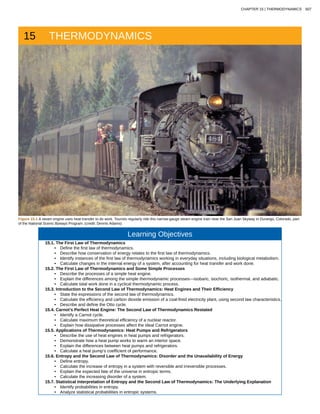
  • 1. 15 THERMODYNAMICS Figure 15.1 A steam engine uses heat transfer to do work. Tourists regularly ride this narrow-gauge steam engine train near the San Juan Skyway in Durango, Colorado, part of the National Scenic Byways Program. (credit: Dennis Adams) Learning Objectives 15.1. The First Law of Thermodynamics • Define the first law of thermodynamics. • Describe how conservation of energy relates to the first law of thermodynamics. • Identify instances of the first law of thermodynamics working in everyday situations, including biological metabolism. • Calculate changes in the internal energy of a system, after accounting for heat transfer and work done. 15.2. The First Law of Thermodynamics and Some Simple Processes • Describe the processes of a simple heat engine. • Explain the differences among the simple thermodynamic processes—isobaric, isochoric, isothermal, and adiabatic. • Calculate total work done in a cyclical thermodynamic process. 15.3. Introduction to the Second Law of Thermodynamics: Heat Engines and Their Efficiency • State the expressions of the second law of thermodynamics. • Calculate the efficiency and carbon dioxide emission of a coal-fired electricity plant, using second law characteristics. • Describe and define the Otto cycle. 15.4. Carnot’s Perfect Heat Engine: The Second Law of Thermodynamics Restated • Identify a Carnot cycle. • Calculate maximum theoretical efficiency of a nuclear reactor. • Explain how dissipative processes affect the ideal Carnot engine. 15.5. Applications of Thermodynamics: Heat Pumps and Refrigerators • Describe the use of heat engines in heat pumps and refrigerators. • Demonstrate how a heat pump works to warm an interior space. • Explain the differences between heat pumps and refrigerators. • Calculate a heat pump’s coefficient of performance. 15.6. Entropy and the Second Law of Thermodynamics: Disorder and the Unavailability of Energy • Define entropy. • Calculate the increase of entropy in a system with reversible and irreversible processes. • Explain the expected fate of the universe in entropic terms. • Calculate the increasing disorder of a system. 15.7. Statistical Interpretation of Entropy and the Second Law of Thermodynamics: The Underlying Explanation • Identify probabilities in entropy. • Analyze statistical probabilities in entropic systems. CHAPTER 15 | THERMODYNAMICS 507
  • 2. Introduction to Thermodynamics Heat transfer is energy in transit, and it can be used to do work. It can also be converted to any other form of energy. A car engine, for example, burns fuel for heat transfer into a gas. Work is done by the gas as it exerts a force through a distance, converting its energy into a variety of other forms—into the car’s kinetic or gravitational potential energy; into electrical energy to run the spark plugs, radio, and lights; and back into stored energy in the car’s battery. But most of the heat transfer produced from burning fuel in the engine does not do work on the gas. Rather, the energy is released into the environment, implying that the engine is quite inefficient. It is often said that modern gasoline engines cannot be made to be significantly more efficient. We hear the same about heat transfer to electrical energy in large power stations, whether they are coal, oil, natural gas, or nuclear powered. Why is that the case? Is the inefficiency caused by design problems that could be solved with better engineering and superior materials? Is it part of some money-making conspiracy by those who sell energy? Actually, the truth is more interesting, and reveals much about the nature of heat transfer. Basic physical laws govern how heat transfer for doing work takes place and place insurmountable limits onto its efficiency. This chapter will explore these laws as well as many applications and concepts associated with them. These topics are part of thermodynamics—the study of heat transfer and its relationship to doing work. 15.1 The First Law of Thermodynamics Figure 15.2 This boiling tea kettle represents energy in motion. The water in the kettle is turning to water vapor because heat is being transferred from the stove to the kettle. As the entire system gets hotter, work is done—from the evaporation of the water to the whistling of the kettle. (credit: Gina Hamilton) If we are interested in how heat transfer is converted into doing work, then the conservation of energy principle is important. The first law of thermodynamics applies the conservation of energy principle to systems where heat transfer and doing work are the methods of transferring energy into and out of the system. The first law of thermodynamics states that the change in internal energy of a system equals the net heat transfer into the system minus the net work done by the system. In equation form, the first law of thermodynamics is (15.1)ΔU = Q − W. Here ΔU is the change in internal energy U of the system. Q is the net heat transferred into the system—that is, Q is the sum of all heat transfer into and out of the system. W is the net work done by the system—that is, W is the sum of all work done on or by the system. We use the following sign conventions: if Q is positive, then there is a net heat transfer into the system; if W is positive, then there is net work done by the system. So positive Q adds energy to the system and positive W takes energy from the system. Thus ΔU = Q − W . Note also that if more heat transfer into the system occurs than work done, the difference is stored as internal energy. Heat engines are a good example of this—heat transfer into them takes place so that they can do work. (See Figure 15.3.) We will now examine Q , W , and ΔU further. 508 CHAPTER 15 | THERMODYNAMICS This content is available for free at http://cnx.org/content/col11406/1.7
  • 3. Figure 15.3 The first law of thermodynamics is the conservation-of-energy principle stated for a system where heat and work are the methods of transferring energy for a system in thermal equilibrium. Q represents the net heat transfer—it is the sum of all heat transfers into and out of the system. Q is positive for net heat transfer into the system. W is the total work done on and by the system. W is positive when more work is done by the system than on it. The change in the internal energy of the system, ΔU , is related to heat and work by the first law of thermodynamics, ΔU = Q − W . Making Connections: Law of Thermodynamics and Law of Conservation of Energy The first law of thermodynamics is actually the law of conservation of energy stated in a form most useful in thermodynamics. The first law gives the relationship between heat transfer, work done, and the change in internal energy of a system. Heat Q and Work W Heat transfer ( Q ) and doing work ( W ) are the two everyday means of bringing energy into or taking energy out of a system. The processes are quite different. Heat transfer, a less organized process, is driven by temperature differences. Work, a quite organized process, involves a macroscopic force exerted through a distance. Nevertheless, heat and work can produce identical results.For example, both can cause a temperature increase. Heat transfer into a system, such as when the Sun warms the air in a bicycle tire, can increase its temperature, and so can work done on the system, as when the bicyclist pumps air into the tire. Once the temperature increase has occurred, it is impossible to tell whether it was caused by heat transfer or by doing work. This uncertainty is an important point. Heat transfer and work are both energy in transit—neither is stored as such in a system. However, both can change the internal energy U of a system. Internal energy is a form of energy completely different from either heat or work. Internal Energy U We can think about the internal energy of a system in two different but consistent ways. The first is the atomic and molecular view, which examines the system on the atomic and molecular scale. The internal energy U of a system is the sum of the kinetic and potential energies of its atoms and molecules. Recall that kinetic plus potential energy is called mechanical energy. Thus internal energy is the sum of atomic and molecular mechanical energy. Because it is impossible to keep track of all individual atoms and molecules, we must deal with averages and distributions. A second way to view the internal energy of a system is in terms of its macroscopic characteristics, which are very similar to atomic and molecular average values. Macroscopically, we define the change in internal energy ΔU to be that given by the first law of thermodynamics: (15.2)ΔU = Q − W. Many detailed experiments have verified that ΔU = Q − W , where ΔU is the change in total kinetic and potential energy of all atoms and molecules in a system. It has also been determined experimentally that the internal energy U of a system depends only on the state of the system and not how it reached that state. More specifically, U is found to be a function of a few macroscopic quantities (pressure, volume, and temperature, for example), independent of past history such as whether there has been heat transfer or work done. This independence means that if we know the state of a system, we can calculate changes in its internal energy U from a few macroscopic variables. Making Connections: Macroscopic and Microscopic In thermodynamics, we often use the macroscopic picture when making calculations of how a system behaves, while the atomic and molecular picture gives underlying explanations in terms of averages and distributions. We shall see this again in later sections of this chapter. For example, in the topic of entropy, calculations will be made using the atomic and molecular view. To get a better idea of how to think about the internal energy of a system, let us examine a system going from State 1 to State 2. The system has internal energy U1 in State 1, and it has internal energy U2 in State 2, no matter how it got to either state. So the change in internal energy ΔU = U2 − U1 is independent of what caused the change. In other words, ΔU is independent of path. By path, we mean the method of getting from the starting point to the ending point. Why is this independence important? Note that ΔU = Q − W . Both Q and W depend on path, but ΔU does not. This path independence means that internal energy U is easier to consider than either heat transfer or work done. CHAPTER 15 | THERMODYNAMICS 509
  • 4. Example 15.1 Calculating Change in Internal Energy: The Same Change in U is Produced by Two Different Processes (a) Suppose there is heat transfer of 40.00 J to a system, while the system does 10.00 J of work. Later, there is heat transfer of 25.00 J out of the system while 4.00 J of work is done on the system. What is the net change in internal energy of the system? (b) What is the change in internal energy of a system when a total of 150.00 J of heat transfer occurs out of (from) the system and 159.00 J of work is done on the system? (See Figure 15.4). Strategy In part (a), we must first find the net heat transfer and net work done from the given information. Then the first law of thermodynamics ⎛ ⎝ΔU = Q − W⎞ ⎠ can be used to find the change in internal energy. In part (b), the net heat transfer and work done are given, so the equation can be used directly. Solution for (a) The net heat transfer is the heat transfer into the system minus the heat transfer out of the system, or (15.3)Q = 40.00 J − 25.00 J = 15.00 J. Similarly, the total work is the work done by the system minus the work done on the system, or (15.4)W = 10.00 J − 4.00 J = 6.00 J. Thus the change in internal energy is given by the first law of thermodynamics: (15.5)ΔU = Q − W = 15.00 J − 6.00 J = 9.00 J. We can also find the change in internal energy for each of the two steps. First, consider 40.00 J of heat transfer in and 10.00 J of work out, or (15.6)ΔU1 = Q1 − W1 = 40.00 J − 10.00 J = 30.00 J. Now consider 25.00 J of heat transfer out and 4.00 J of work in, or (15.7)ΔU2 = Q2 − W2= - 25.00 J − ( − 4.00 J ) = –21.00 J. The total change is the sum of these two steps, or (15.8)ΔU = ΔU1 + ΔU2 = 30.00 J + (−21.00 J ) = 9.00 J. Discussion on (a) No matter whether you look at the overall process or break it into steps, the change in internal energy is the same. Solution for (b) Here the net heat transfer and total work are given directly to be Q = – 150.00 J and W = – 159.00 J , so that (15.9)ΔU = Q – W = – 150.00 J – ( − 159.00 J) = 9.00 J. Discussion on (b) A very different process in part (b) produces the same 9.00-J change in internal energy as in part (a). Note that the change in the system in both parts is related to ΔU and not to the individual Q s or W s involved. The system ends up in the same state in both (a) and (b). Parts (a) and (b) present two different paths for the system to follow between the same starting and ending points, and the change in internal energy for each is the same—it is independent of path. 510 CHAPTER 15 | THERMODYNAMICS This content is available for free at http://cnx.org/content/col11406/1.7
  • 5. Figure 15.4 Two different processes produce the same change in a system. (a) A total of 15.00 J of heat transfer occurs into the system, while work takes out a total of 6.00 J. The change in internal energy is ΔU = Q − W = 9.00 J . (b) Heat transfer removes 150.00 J from the system while work puts 159.00 J into it, producing an increase of 9.00 J in internal energy. If the system starts out in the same state in (a) and (b), it will end up in the same final state in either case—its final state is related to internal energy, not how that energy was acquired. Human Metabolism and the First Law of Thermodynamics Human metabolism is the conversion of food into heat transfer, work, and stored fat. Metabolism is an interesting example of the first law of thermodynamics in action. We now take another look at these topics via the first law of thermodynamics. Considering the body as the system of interest, we can use the first law to examine heat transfer, doing work, and internal energy in activities ranging from sleep to heavy exercise. What are some of the major characteristics of heat transfer, doing work, and energy in the body? For one, body temperature is normally kept constant by heat transfer to the surroundings. This means Q is negative. Another fact is that the body usually does work on the outside world. This means W is positive. In such situations, then, the body loses internal energy, since ΔU = Q − W is negative. Now consider the effects of eating. Eating increases the internal energy of the body by adding chemical potential energy (this is an unromantic view of a good steak). The body metabolizes all the food we consume. Basically, metabolism is an oxidation process in which the chemical potential energy of food is released. This implies that food input is in the form of work. Food energy is reported in a special unit, known as the Calorie. This energy is measured by burning food in a calorimeter, which is how the units are determined. In chemistry and biochemistry, one calorie (spelled with a lowercase c) is defined as the energy (or heat transfer) required to raise the temperature of one gram of pure water by one degree Celsius. Nutritionists and weight-watchers tend to use the dietary calorie, which is frequently called a Calorie (spelled with a capital C). One food Calorie is the energy needed to raise the temperature of one kilogram of water by one degree Celsius. This means that one dietary Calorie is equal to one kilocalorie for the chemist, and one must be careful to avoid confusion between the two. Again, consider the internal energy the body has lost. There are three places this internal energy can go—to heat transfer, to doing work, and to stored fat (a tiny fraction also goes to cell repair and growth). Heat transfer and doing work take internal energy out of the body, and food puts it back. If you eat just the right amount of food, then your average internal energy remains constant. Whatever you lose to heat transfer and doing work is replaced by food, so that, in the long run, ΔU = 0 . If you overeat repeatedly, then ΔU is always positive, and your body stores this extra internal energy as fat. The reverse is true if you eat too little. If ΔU is negative for a few days, then the body metabolizes its own fat to maintain body temperature and do work that takes energy from the body. This process is how dieting produces weight loss. Life is not always this simple, as any dieter knows. The body stores fat or metabolizes it only if energy intake changes for a period of several days. Once you have been on a major diet, the next one is less successful because your body alters the way it responds to low energy intake. Your basal metabolic rate (BMR) is the rate at which food is converted into heat transfer and work done while the body is at complete rest. The body adjusts its basal metabolic rate to partially compensate for over-eating or under-eating. The body will decrease the metabolic rate rather than eliminate its own fat to replace lost food intake. You will chill more easily and feel less energetic as a result of the lower metabolic rate, and you will not lose weight as fast as before. Exercise helps to lose weight, because it produces both heat transfer from your body and work, and raises your metabolic rate even when you are at rest. Weight loss is also aided by the quite low efficiency of the body in converting internal energy to work, so that the loss of internal energy resulting from doing work is much greater than the work done.It should be noted, however, that living systems are not in thermalequilibrium. The body provides us with an excellent indication that many thermodynamic processes are irreversible. An irreversible process can go in one direction but not the reverse, under a given set of conditions. For example, although body fat can be converted to do work and produce heat transfer, CHAPTER 15 | THERMODYNAMICS 511
  • 6. work done on the body and heat transfer into it cannot be converted to body fat. Otherwise, we could skip lunch by sunning ourselves or by walking down stairs. Another example of an irreversible thermodynamic process is photosynthesis. This process is the intake of one form of energy—light—by plants and its conversion to chemical potential energy. Both applications of the first law of thermodynamics are illustrated in Figure 15.5. One great advantage of conservation laws such as the first law of thermodynamics is that they accurately describe the beginning and ending points of complex processes, such as metabolism and photosynthesis, without regard to the complications in between. Table 15.1 presents a summary of terms relevant to the first law of thermodynamics. Figure 15.5 (a) The first law of thermodynamics applied to metabolism. Heat transferred out of the body ( Q ) and work done by the body ( W ) remove internal energy, while food intake replaces it. (Food intake may be considered as work done on the body.) (b) Plants convert part of the radiant heat transfer in sunlight to stored chemical energy, a process called photosynthesis. Table 15.1 Summary of Terms for the First Law of Thermodynamics, ΔU=Q−W Term Definition U Internal energy—the sum of the kinetic and potential energies of a system’s atoms and molecules. Can be divided into many subcategories, such as thermal and chemical energy. Depends only on the state of a system (such as its P , V , and T ), not on how the energy entered the system. Change in internal energy is path independent. Q Heat—energy transferred because of a temperature difference. Characterized by random molecular motion. Highly dependent on path. Q entering a system is positive. W Work—energy transferred by a force moving through a distance. An organized, orderly process. Path dependent. W done by a system (either against an external force or to increase the volume of the system) is positive. 15.2 The First Law of Thermodynamics and Some Simple Processes Figure 15.6 Beginning with the Industrial Revolution, humans have harnessed power through the use of the first law of thermodynamics, before we even understood it completely. This photo, of a steam engine at the Turbinia Works, dates from 1911, a mere 61 years after the first explicit statement of the first law of thermodynamics by Rudolph Clausius. (credit: public domain; author unknown) One of the most important things we can do with heat transfer is to use it to do work for us. Such a device is called a heat engine. Car engines and steam turbines that generate electricity are examples of heat engines. Figure 15.7 shows schematically how the first law of thermodynamics applies to the typical heat engine. 512 CHAPTER 15 | THERMODYNAMICS This content is available for free at http://cnx.org/content/col11406/1.7
  • 7. Figure 15.7 Schematic representation of a heat engine, governed, of course, by the first law of thermodynamics. It is impossible to devise a system where Qout = 0 , that is, in which no heat transfer occurs to the environment. Figure 15.8 (a) Heat transfer to the gas in a cylinder increases the internal energy of the gas, creating higher pressure and temperature. (b) The force exerted on the movable cylinder does work as the gas expands. Gas pressure and temperature decrease when it expands, indicating that the gas’s internal energy has been decreased by doing work. (c) Heat transfer to the environment further reduces pressure in the gas so that the piston can be more easily returned to its starting position. The illustrations above show one of the ways in which heat transfer does work. Fuel combustion produces heat transfer to a gas in a cylinder, increasing the pressure of the gas and thereby the force it exerts on a movable piston. The gas does work on the outside world, as this force moves the piston through some distance. Heat transfer to the gas cylinder results in work being done. To repeat this process, the piston needs to be returned to its starting point. Heat transfer now occurs from the gas to the surroundings so that its pressure decreases, and a force is exerted by the surroundings to push the piston back through some distance. Variations of this process are employed daily in hundreds of millions of heat engines. We will examine heat engines in detail in the next section. In this section, we consider some of the simpler underlying processes on which heat engines are based. CHAPTER 15 | THERMODYNAMICS 513
  • 8. PV Diagrams and their Relationship to Work Done on or by a Gas A process by which a gas does work on a piston at constant pressure is called an isobaric process. Since the pressure is constant, the force exerted is constant and the work done is given as (15.10)PΔV. Figure 15.9 An isobaric expansion of a gas requires heat transfer to keep the pressure constant. Since pressure is constant, the work done is PΔV . (15.11)W = Fd See the symbols as shown in Figure 15.9. Now F = PA , and so (15.12)W = PAd. Because the volume of a cylinder is its cross-sectional area A times its length d , we see that Ad = ΔV , the change in volume; thus, (15.13)W = PΔV (isobaric process). Note that if ΔV is positive, then W is positive, meaning that work is done by the gas on the outside world. (Note that the pressure involved in this work that we’ve called P is the pressure of the gas inside the tank. If we call the pressure outside the tank Pext , an expanding gas would be working against the external pressure; the work done would therefore be W = −PextΔV (isobaric process). Many texts use this definition of work, and not the definition based on internal pressure, as the basis of the First Law of Thermodynamics. This definition reverses the sign conventions for work, and results in a statement of the first law that becomes ΔU = Q + W .) It is not surprising that W = PΔV , since we have already noted in our treatment of fluids that pressure is a type of potential energy per unit volume and that pressure in fact has units of energy divided by volume. We also noted in our discussion of the ideal gas law that PV has units of energy. In this case, some of the energy associated with pressure becomes work. Figure 15.10 shows a graph of pressure versus volume (that is, a PV diagram for an isobaric process. You can see in the figure that the work done is the area under the graph. This property of PV diagrams is very useful and broadly applicable: the work done on or by a system in going from one state to another equals the area under the curve on a PV diagram. 514 CHAPTER 15 | THERMODYNAMICS This content is available for free at http://cnx.org/content/col11406/1.7
  • 9. Figure 15.10 A graph of pressure versus volume for a constant-pressure, or isobaric, process, such as the one shown in Figure 15.9. The area under the curve equals the work done by the gas, since W = PΔV . Figure 15.11 (a) A PV diagram in which pressure varies as well as volume. The work done for each interval is its average pressure times the change in volume, or the area under the curve over that interval. Thus the total area under the curve equals the total work done. (b) Work must be done on the system to follow the reverse path. This is interpreted as a negative area under the curve. We can see where this leads by considering Figure 15.11(a), which shows a more general process in which both pressure and volume change. The area under the curve is closely approximated by dividing it into strips, each having an average constant pressure Pi(ave) . The work done is Wi = Pi(ave)ΔVi for each strip, and the total work done is the sum of the Wi . Thus the total work done is the total area under the curve. If the path is reversed, as in Figure 15.11(b), then work is done on the system. The area under the curve in that case is negative, because ΔV is negative. PV diagrams clearly illustrate that the work done depends on the path taken and not just the endpoints. This path dependence is seen in Figure 15.12(a), where more work is done in going from A to C by the path via point B than by the path via point D. The vertical paths, where volume is constant, are called isochoric processes. Since volume is constant, ΔV = 0 , and no work is done in an isochoric process. Now, if the system follows the cyclical path ABCDA, as in Figure 15.12(b), then the total work done is the area inside the loop. The negative area below path CD subtracts, leaving only the area inside the rectangle. In fact, the work done in any cyclical process (one that returns to its starting point) is the area inside the loop it forms on a PV diagram, as Figure 15.12(c) illustrates for a general cyclical process. Note that the loop must be traversed in the clockwise direction for work to be positive—that is, for there to be a net work output. CHAPTER 15 | THERMODYNAMICS 515
  • 10. Figure 15.12 (a) The work done in going from A to C depends on path. The work is greater for the path ABC than for the path ADC, because the former is at higher pressure. In both cases, the work done is the area under the path. This area is greater for path ABC. (b) The total work done in the cyclical process ABCDA is the area inside the loop, since the negative area below CD subtracts out, leaving just the area inside the rectangle. (The values given for the pressures and the change in volume are intended for use in the example below.) (c) The area inside any closed loop is the work done in the cyclical process. If the loop is traversed in a clockwise direction, W is positive—it is work done on the outside environment. If the loop is traveled in a counter-clockwise direction, W is negative—it is work that is done to the system. Example 15.2 Total Work Done in a Cyclical Process Equals the Area Inside the Closed Loop on a PV Diagram Calculate the total work done in the cyclical process ABCDA shown in Figure 15.12(b) by the following two methods to verify that work equals the area inside the closed loop on the PV diagram. (Take the data in the figure to be precise to three significant figures.) (a) Calculate the work done along each segment of the path and add these values to get the total work. (b) Calculate the area inside the rectangle ABCDA. Strategy To find the work along any path on a PV diagram, you use the fact that work is pressure times change in volume, or W = PΔV . So in part (a), this value is calculated for each leg of the path around the closed loop. Solution for (a) The work along path AB is (15.14)WAB = PABΔVAB = (1.50×10⁶ N/m2 )(5.00×10⁻⁴ m3 ) = 750 J. Since the path BC is isochoric, ΔVBC = 0 , and so WBC = 0 . The work along path CD is negative, since ΔVCD is negative (the volume decreases). The work is 516 CHAPTER 15 | THERMODYNAMICS This content is available for free at http://cnx.org/content/col11406/1.7
  • 11. (15.15)WCD = PCDΔVCD = (2.00×10⁵ N/m2 )(–5.00×10⁻⁴ m3 ) = –100 J. Again, since the path DA is isochoric, ΔVDA = 0 , and so WDA = 0 . Now the total work is (15.16)W = WAB + WBC + WCD + WDA = 750 J+0 + ( − 100J) + 0 = 650 J. Solution for (b) The area inside the rectangle is its height times its width, or (15.17)area = (PAB − PCD)ΔV = ⎡ ⎣(1.50×10⁶ N/m2 ) − (2.00×10⁵ N/m2 )⎤ ⎦(5.00×10⁻⁴ m3 ) = 650 J. Thus, (15.18)area = 650 J = W. Discussion The result, as anticipated, is that the area inside the closed loop equals the work done. The area is often easier to calculate than is the work done along each path. It is also convenient to visualize the area inside different curves on PV diagrams in order to see which processes might produce the most work. Recall that work can be done to the system, or by the system, depending on the sign of W . A positive W is work that is done by the system on the outside environment; a negative W represents work done by the environment on the system. Figure 15.13(a) shows two other important processes on a PV diagram. For comparison, both are shown starting from the same point A. The upper curve ending at point B is an isothermal process—that is, one in which temperature is kept constant. If the gas behaves like an ideal gas, as is often the case, and if no phase change occurs, then PV = nRT . Since T is constant, PV is a constant for an isothermal process. We ordinarily expect the temperature of a gas to decrease as it expands, and so we correctly suspect that heat transfer must occur from the surroundings to the gas to keep the temperature constant during an isothermal expansion. To show this more rigorously for the special case of a monatomic ideal gas, we note that the average kinetic energy of an atom in such a gas is given by (15.19)1 2 m v¯ 2 = 3 2 kT. The kinetic energy of the atoms in a monatomic ideal gas is its only form of internal energy, and so its total internal energy U is (15.20) U = N1 2 m v¯ 2 = 3 2 NkT, (monatomic ideal gas), where N is the number of atoms in the gas. This relationship means that the internal energy of an ideal monatomic gas is constant during an isothermal process—that is, ΔU = 0 . If the internal energy does not change, then the net heat transfer into the gas must equal the net work done by the gas. That is, because ΔU = Q − W = 0 here, Q = W . We must have just enough heat transfer to replace the work done. An isothermal process is inherently slow, because heat transfer occurs continuously to keep the gas temperature constant at all times and must be allowed to spread through the gas so that there are no hot or cold regions. Also shown in Figure 15.13(a) is a curve AC for an adiabatic process, defined to be one in which there is no heat transfer—that is, Q = 0 . Processes that are nearly adiabatic can be achieved either by using very effective insulation or by performing the process so fast that there is little time for heat transfer. Temperature must decrease during an adiabatic process, since work is done at the expense of internal energy: (15.21) U = 3 2 NkT. (You might have noted that a gas released into atmospheric pressure from a pressurized cylinder is substantially colder than the gas in the cylinder.) In fact, because Q = 0, ΔU = – W for an adiabatic process. Lower temperature results in lower pressure along the way, so that curve AC is lower than curve AB, and less work is done. If the path ABCA could be followed by cooling the gas from B to C at constant volume (isochorically), Figure 15.13(b), there would be a net work output. CHAPTER 15 | THERMODYNAMICS 517
  • 12. Figure 15.13 (a) The upper curve is an isothermal process ( ΔT = 0 ), whereas the lower curve is an adiabatic process ( Q = 0 ). Both start from the same point A, but the isothermal process does more work than the adiabatic because heat transfer into the gas takes place to keep its temperature constant. This keeps the pressure higher all along the isothermal path than along the adiabatic path, producing more work. The adiabatic path thus ends up with a lower pressure and temperature at point C, even though the final volume is the same as for the isothermal process. (b) The cycle ABCA produces a net work output. Reversible Processes Both isothermal and adiabatic processes such as shown in Figure 15.13 are reversible in principle. A reversible process is one in which both the system and its environment can return to exactly the states they were in by following the reverse path. The reverse isothermal and adiabatic paths are BA and CA, respectively. Real macroscopic processes are never exactly reversible. In the previous examples, our system is a gas (like that in Figure 15.9), and its environment is the piston, cylinder, and the rest of the universe. If there are any energy-dissipating mechanisms, such as friction or turbulence, then heat transfer to the environment occurs for either direction of the piston. So, for example, if the path BA is followed and there is friction, then the gas will be returned to its original state but the environment will not—it will have been heated in both directions. Reversibility requires the direction of heat transfer to reverse for the reverse path. Since dissipative mechanisms cannot be completely eliminated, real processes cannot be reversible. There must be reasons that real macroscopic processes cannot be reversible. We can imagine them going in reverse. For example, heat transfer occurs spontaneously from hot to cold and never spontaneously the reverse. Yet it would not violate the first law of thermodynamics for this to happen. In fact, all spontaneous processes, such as bubbles bursting, never go in reverse. There is a second thermodynamic law that forbids them from going in reverse. When we study this law, we will learn something about nature and also find that such a law limits the efficiency of heat engines. We will find that heat engines with the greatest possible theoretical efficiency would have to use reversible processes, and even they cannot convert all heat transfer into doing work. Table 15.2 summarizes the simpler thermodynamic processes and their definitions. Table 15.2 Summary of Simple Thermodynamic Processes Isobaric Constant pressure W = PΔV Isochoric Constant volume W = 0 Isothermal Constant temperature Q = W Adiabatic No heat transfer Q = 0 PhET Explorations: States of Matter Watch different types of molecules form a solid, liquid, or gas. Add or remove heat and watch the phase change. Change the temperature or volume of a container and see a pressure-temperature diagram respond in real time. Relate the interaction potential to the forces between molecules. 518 CHAPTER 15 | THERMODYNAMICS This content is available for free at http://cnx.org/content/col11406/1.7
  • 13. Figure 15.14 States of Matter (http://cnx.org/content/m42233/1.5/states-of-matter_en.jar) 15.3 Introduction to the Second Law of Thermodynamics: Heat Engines and Their Efficiency Figure 15.15 These ice floes melt during the Arctic summer. Some of them refreeze in the winter, but the second law of thermodynamics predicts that it would be extremely unlikely for the water molecules contained in these particular floes to reform the distinctive alligator-like shape they formed when the picture was taken in the summer of 2009. (credit: Patrick Kelley, U.S. Coast Guard, U.S. Geological Survey) The second law of thermodynamics deals with the direction taken by spontaneous processes. Many processes occur spontaneously in one direction only—that is, they are irreversible, under a given set of conditions. Although irreversibility is seen in day-to-day life—a broken glass does not resume its original state, for instance—complete irreversibility is a statistical statement that cannot be seen during the lifetime of the universe. More precisely, an irreversible process is one that depends on path. If the process can go in only one direction, then the reverse path differs fundamentally and the process cannot be reversible. For example, as noted in the previous section, heat involves the transfer of energy from higher to lower temperature. A cold object in contact with a hot one never gets colder, transferring heat to the hot object and making it hotter. Furthermore, mechanical energy, such as kinetic energy, can be completely converted to thermal energy by friction, but the reverse is impossible. A hot stationary object never spontaneously cools off and starts moving. Yet another example is the expansion of a puff of gas introduced into one corner of a vacuum chamber. The gas expands to fill the chamber, but it never regroups in the corner. The random motion of the gas molecules could take them all back to the corner, but this is never observed to happen. (See Figure 15.16.) CHAPTER 15 | THERMODYNAMICS 519
  • 14. Figure 15.16 Examples of one-way processes in nature. (a) Heat transfer occurs spontaneously from hot to cold and not from cold to hot. (b) The brakes of this car convert its kinetic energy to heat transfer to the environment. The reverse process is impossible. (c) The burst of gas let into this vacuum chamber quickly expands to uniformly fill every part of the chamber. The random motions of the gas molecules will never return them to the corner. The fact that certain processes never occur suggests that there is a law forbidding them to occur. The first law of thermodynamics would allow them to occur—none of those processes violate conservation of energy. The law that forbids these processes is called the second law of thermodynamics. We shall see that the second law can be stated in many ways that may seem different, but which in fact are equivalent. Like all natural laws, the second law of thermodynamics gives insights into nature, and its several statements imply that it is broadly applicable, fundamentally affecting many apparently disparate processes. The already familiar direction of heat transfer from hot to cold is the basis of our first version of the second law of thermodynamics. The Second Law of Thermodynamics (first expression) Heat transfer occurs spontaneously from higher- to lower-temperature bodies but never spontaneously in the reverse direction. Another way of stating this: It is impossible for any process to have as its sole result heat transfer from a cooler to a hotter object. Heat Engines Now let us consider a device that uses heat transfer to do work. As noted in the previous section, such a device is called a heat engine, and one is shown schematically in Figure 15.17(b). Gasoline and diesel engines, jet engines, and steam turbines are all heat engines that do work by using part of the heat transfer from some source. Heat transfer from the hot object (or hot reservoir) is denoted as Qh , while heat transfer into the cold object (or cold reservoir) is Qc , and the work done by the engine is W . The temperatures of the hot and cold reservoirs are Th and Tc , respectively. 520 CHAPTER 15 | THERMODYNAMICS This content is available for free at http://cnx.org/content/col11406/1.7
  • 15. Figure 15.17 (a) Heat transfer occurs spontaneously from a hot object to a cold one, consistent with the second law of thermodynamics. (b) A heat engine, represented here by a circle, uses part of the heat transfer to do work. The hot and cold objects are called the hot and cold reservoirs. Qh is the heat transfer out of the hot reservoir, W is the work output, and Qc is the heat transfer into the cold reservoir. Because the hot reservoir is heated externally, which is energy intensive, it is important that the work is done as efficiently as possible. In fact, we would like W to equal Qh , and for there to be no heat transfer to the environment ( Qc = 0 ). Unfortunately, this is impossible. The second law of thermodynamics also states, with regard to using heat transfer to do work (the second expression of the second law): The Second Law of Thermodynamics (second expression) It is impossible in any system for heat transfer from a reservoir to completely convert to work in a cyclical process in which the system returns to its initial state. A cyclical process brings a system, such as the gas in a cylinder, back to its original state at the end of every cycle. Most heat engines, such as reciprocating piston engines and rotating turbines, use cyclical processes. The second law, just stated in its second form, clearly states that such engines cannot have perfect conversion of heat transfer into work done. Before going into the underlying reasons for the limits on converting heat transfer into work, we need to explore the relationships among W , Qh , and Qc , and to define the efficiency of a cyclical heat engine. As noted, a cyclical process brings the system back to its original condition at the end of every cycle. Such a system’s internal energy U is the same at the beginning and end of every cycle—that is, ΔU = 0 . The first law of thermodynamics states that (15.22)ΔU = Q − W, where Q is the net heat transfer during the cycle ( Q = Qh − Qc ) and W is the net work done by the system. Since ΔU = 0 for a complete cycle, we have (15.23)0 = Q − W, so that (15.24)W = Q. Thus the net work done by the system equals the net heat transfer into the system, or (15.25)W = Qh − Qc (cyclical process), just as shown schematically in Figure 15.17(b). The problem is that in all processes, there is some heat transfer Qc to the environment—and usually a very significant amount at that. In the conversion of energy to work, we are always faced with the problem of getting less out than we put in. We define conversion efficiency Eff to be the ratio of useful work output to the energy input (or, in other words, the ratio of what we get to what we spend). In that spirit, we define the efficiency of a heat engine to be its net work output W divided by heat transfer to the engine Qh ; that is, (15.26) Eff = W Qh . Since W = Qh − Qc in a cyclical process, we can also express this as (15.27) Eff = Qh − Qc Qh = 1 − Qc Qh (cyclical process), CHAPTER 15 | THERMODYNAMICS 521
  • 16. making it clear that an efficiency of 1, or 100%, is possible only if there is no heat transfer to the environment ( Qc = 0 ). Note that all Q s are positive. The direction of heat transfer is indicated by a plus or minus sign. For example, Qc is out of the system and so is preceded by a minus sign. Example 15.3 Daily Work Done by a Coal-Fired Power Station, Its Efficiency and Carbon Dioxide Emissions A coal-fired power station is a huge heat engine. It uses heat transfer from burning coal to do work to turn turbines, which are used to generate electricity. In a single day, a large coal power station has 2.50×10¹⁴ J of heat transfer from coal and 1.48×10¹⁴ J of heat transfer into the environment. (a) What is the work done by the power station? (b) What is the efficiency of the power station? (c) In the combustion process, the following chemical reaction occurs: C + O2 → CO2 . This implies that every 12 kg of coal puts 12 kg + 16 kg + 16 kg = 44 kg of carbon dioxide into the atmosphere. Assuming that 1 kg of coal can provide 2.5×10⁶ J of heat transfer upon combustion, how much CO2 is emitted per day by this power plant? Strategy for (a) We can use W = Qh − Qc to find the work output W , assuming a cyclical process is used in the power station. In this process, water is boiled under pressure to form high-temperature steam, which is used to run steam turbine-generators, and then condensed back to water to start the cycle again. Solution for (a) Work output is given by: (15.28)W = Qh − Qc. Substituting the given values: (15.29)W = 2.50×10¹⁴ J – 1.48×10¹⁴ J = 1.02×10¹⁴ J. Strategy for (b) The efficiency can be calculated with Eff = W Qh since Qh is given and work W was found in the first part of this example. Solution for (b) Efficiency is given by: Eff = W Qh . The work W was just found to be 1.02 × 10¹⁴ J , and Qh is given, so the efficiency is (15.30) Eff = 1.02×10¹⁴ J 2.50×10¹⁴ J = 0.408, or 40.8% Strategy for (c) The daily consumption of coal is calculated using the information that each day there is 2.50×10¹⁴ J of heat transfer from coal. In the combustion process, we have C + O2 → CO2 . So every 12 kg of coal puts 12 kg + 16 kg + 16 kg = 44 kg of CO2 into the atmosphere. Solution for (c) The daily coal consumption is (15.31)2.50×10¹⁴ J 2.50×10⁶ J/kg = 1.0×10⁸ kg. Assuming that the coal is pure and that all the coal goes toward producing carbon dioxide, the carbon dioxide produced per day is (15.32) 1.0×10⁸ kg coal× 44 kg CO2 12 kg coal = 3.7×10⁸ kg CO2. This is 370,000 metric tons of CO2 produced every day. Discussion If all the work output is converted to electricity in a period of one day, the average power output is 1180 MW (this is left to you as an end-of- chapter problem). This value is about the size of a large-scale conventional power plant. The efficiency found is acceptably close to the value of 42% given for coal power stations. It means that fully 59.2% of the energy is heat transfer to the environment, which usually results in warming lakes, rivers, or the ocean near the power station, and is implicated in a warming planet generally. While the laws of thermodynamics limit the efficiency of such plants—including plants fired by nuclear fuel, oil, and natural gas—the heat transfer to the environment could be, and sometimes is, used for heating homes or for industrial processes. The generally low cost of energy has not made it economical to make better use of the waste heat transfer from most heat engines. Coal-fired power plants produce the greatest amount of CO2 per unit energy output (compared to natural gas or oil), making coal the least efficient fossil fuel. 522 CHAPTER 15 | THERMODYNAMICS This content is available for free at http://cnx.org/content/col11406/1.7
  • 17. With the information given in Example 15.3, we can find characteristics such as the efficiency of a heat engine without any knowledge of how the heat engine operates, but looking further into the mechanism of the engine will give us greater insight. Figure 15.18 illustrates the operation of the common four-stroke gasoline engine. The four steps shown complete this heat engine’s cycle, bringing the gasoline-air mixture back to its original condition. The Otto cycle shown in Figure 15.19(a) is used in four-stroke internal combustion engines, although in fact the true Otto cycle paths do not correspond exactly to the strokes of the engine. The adiabatic process AB corresponds to the nearly adiabatic compression stroke of the gasoline engine. In both cases, work is done on the system (the gas mixture in the cylinder), increasing its temperature and pressure. Along path BC of the Otto cycle, heat transfer Qh into the gas occurs at constant volume, causing a further increase in pressure and temperature. This process corresponds to burning fuel in an internal combustion engine, and takes place so rapidly that the volume is nearly constant. Path CD in the Otto cycle is an adiabatic expansion that does work on the outside world, just as the power stroke of an internal combustion engine does in its nearly adiabatic expansion. The work done by the system along path CD is greater than the work done on the system along path AB, because the pressure is greater, and so there is a net work output. Along path DA in the Otto cycle, heat transfer Qc from the gas at constant volume reduces its temperature and pressure, returning it to its original state. In an internal combustion engine, this process corresponds to the exhaust of hot gases and the intake of an air-gasoline mixture at a considerably lower temperature. In both cases, heat transfer into the environment occurs along this final path. The net work done by a cyclical process is the area inside the closed path on a PV diagram, such as that inside path ABCDA in Figure 15.19. Note that in every imaginable cyclical process, it is absolutely necessary for heat transfer from the system to occur in order to get a net work output. In the Otto cycle, heat transfer occurs along path DA. If no heat transfer occurs, then the return path is the same, and the net work output is zero. The lower the temperature on the path AB, the less work has to be done to compress the gas. The area inside the closed path is then greater, and so the engine does more work and is thus more efficient. Similarly, the higher the temperature along path CD, the more work output there is. (See Figure 15.20.) So efficiency is related to the temperatures of the hot and cold reservoirs. In the next section, we shall see what the absolute limit to the efficiency of a heat engine is, and how it is related to temperature. Figure 15.18 In the four-stroke internal combustion gasoline engine, heat transfer into work takes place in the cyclical process shown here. The piston is connected to a rotating crankshaft, which both takes work out of and does work on the gas in the cylinder. (a) Air is mixed with fuel during the intake stroke. (b) During the compression stroke, the air-fuel mixture is rapidly compressed in a nearly adiabatic process, as the piston rises with the valves closed. Work is done on the gas. (c) The power stroke has two distinct parts. First, the air-fuel mixture is ignited, converting chemical potential energy into thermal energy almost instantaneously, which leads to a great increase in pressure. Then the piston descends, and the gas does work by exerting a force through a distance in a nearly adiabatic process. (d) The exhaust stroke expels the hot gas to prepare the engine for another cycle, starting again with the intake stroke. Figure 15.19 PV diagram for a simplified Otto cycle, analogous to that employed in an internal combustion engine. Point A corresponds to the start of the compression stroke of an internal combustion engine. Paths AB and CD are adiabatic and correspond to the compression and power strokes of an internal combustion engine, respectively. Paths BC and DA are isochoric and accomplish similar results to the ignition and exhaust-intake portions, respectively, of the internal combustion engine’s cycle. Work is done on the gas along path AB, but more work is done by the gas along path CD, so that there is a net work output. CHAPTER 15 | THERMODYNAMICS 523
  • 18. Figure 15.20 This Otto cycle produces a greater work output than the one in Figure 15.19, because the starting temperature of path CD is higher and the starting temperature of path AB is lower. The area inside the loop is greater, corresponding to greater net work output. 15.4 Carnot’s Perfect Heat Engine: The Second Law of Thermodynamics Restated Figure 15.21 This novelty toy, known as the drinking bird, is an example of Carnot’s engine. It contains methylene chloride (mixed with a dye) in the abdomen, which boils at a very low temperature—about 100ºF . To operate, one gets the bird’s head wet. As the water evaporates, fluid moves up into the head, causing the bird to become top-heavy and dip forward back into the water. This cools down the methylene chloride in the head, and it moves back into the abdomen, causing the bird to become bottom heavy and tip up. Except for a very small input of energy—the original head-wetting—the bird becomes a perpetual motion machine of sorts. (credit: Arabesk.nl, Wikimedia Commons) We know from the second law of thermodynamics that a heat engine cannot be 100% efficient, since there must always be some heat transfer Qc to the environment, which is often called waste heat. How efficient, then, can a heat engine be? This question was answered at a theoretical level in 1824 by a young French engineer, Sadi Carnot (1796–1832), in his study of the then-emerging heat engine technology crucial to the Industrial Revolution. He devised a theoretical cycle, now called the Carnot cycle, which is the most efficient cyclical process possible. The second law of thermodynamics can be restated in terms of the Carnot cycle, and so what Carnot actually discovered was this fundamental law. Any heat engine employing the Carnot cycle is called a Carnot engine. What is crucial to the Carnot cycle—and, in fact, defines it—is that only reversible processes are used. Irreversible processes involve dissipative factors, such as friction and turbulence. This increases heat transfer Qc to the environment and reduces the efficiency of the engine. Obviously, then, reversible processes are superior. Carnot Engine Stated in terms of reversible processes, the second law of thermodynamics has a third form: A Carnot engine operating between two given temperatures has the greatest possible efficiency of any heat engine operating between these two temperatures. Furthermore, all engines employing only reversible processes have this same maximum efficiency when operating between the same given temperatures. Figure 15.22 shows the PV diagram for a Carnot cycle. The cycle comprises two isothermal and two adiabatic processes. Recall that both isothermal and adiabatic processes are, in principle, reversible. Carnot also determined the efficiency of a perfect heat engine—that is, a Carnot engine. It is always true that the efficiency of a cyclical heat engine is given by: 524 CHAPTER 15 | THERMODYNAMICS This content is available for free at http://cnx.org/content/col11406/1.7
  • 19. (15.33) Eff = Qh − Qc Qh = 1 − Qc Qh . What Carnot found was that for a perfect heat engine, the ratio Qc / Qh equals the ratio of the absolute temperatures of the heat reservoirs. That is, Qc / Qh = Tc / Th for a Carnot engine, so that the maximum or Carnot efficiency EffC is given by (15.34) EffC = 1 − Tc Th , where Th and Tc are in kelvins (or any other absolute temperature scale). No real heat engine can do as well as the Carnot efficiency—an actual efficiency of about 0.7 of this maximum is usually the best that can be accomplished. But the ideal Carnot engine, like the drinking bird above, while a fascinating novelty, has zero power. This makes it unrealistic for any applications. Carnot’s interesting result implies that 100% efficiency would be possible only if Tc = 0 K —that is, only if the cold reservoir were at absolute zero, a practical and theoretical impossibility. But the physical implication is this—the only way to have all heat transfer go into doing work is to remove all thermal energy, and this requires a cold reservoir at absolute zero. It is also apparent that the greatest efficiencies are obtained when the ratio Tc / Th is as small as possible. Just as discussed for the Otto cycle in the previous section, this means that efficiency is greatest for the highest possible temperature of the hot reservoir and lowest possible temperature of the cold reservoir. (This setup increases the area inside the closed loop on the PV diagram; also, it seems reasonable that the greater the temperature difference, the easier it is to divert the heat transfer to work.) The actual reservoir temperatures of a heat engine are usually related to the type of heat source and the temperature of the environment into which heat transfer occurs. Consider the following example. Figure 15.22 PV diagram for a Carnot cycle, employing only reversible isothermal and adiabatic processes. Heat transfer Qh occurs into the working substance during the isothermal path AB, which takes place at constant temperature Th . Heat transfer Qc occurs out of the working substance during the isothermal path CD, which takes place at constant temperature Tc . The net work output W equals the area inside the path ABCDA. Also shown is a schematic of a Carnot engine operating between hot and cold reservoirs at temperatures Th and Tc . Any heat engine using reversible processes and operating between these two temperatures will have the same maximum efficiency as the Carnot engine. Example 15.4 Maximum Theoretical Efficiency for a Nuclear Reactor A nuclear power reactor has pressurized water at 300ºC . (Higher temperatures are theoretically possible but practically not, due to limitations with materials used in the reactor.) Heat transfer from this water is a complex process (see Figure 15.23). Steam, produced in the steam generator, is used to drive the turbine-generators. Eventually the steam is condensed to water at 27ºC and then heated again to start the cycle over. Calculate the maximum theoretical efficiency for a heat engine operating between these two temperatures. CHAPTER 15 | THERMODYNAMICS 525
  • 20. Figure 15.23 Schematic diagram of a pressurized water nuclear reactor and the steam turbines that convert work into electrical energy. Heat exchange is used to generate steam, in part to avoid contamination of the generators with radioactivity. Two turbines are used because this is less expensive than operating a single generator that produces the same amount of electrical energy. The steam is condensed to liquid before being returned to the heat exchanger, to keep exit steam pressure low and aid the flow of steam through the turbines (equivalent to using a lower-temperature cold reservoir). The considerable energy associated with condensation must be dissipated into the local environment; in this example, a cooling tower is used so there is no direct heat transfer to an aquatic environment. (Note that the water going to the cooling tower does not come into contact with the steam flowing over the turbines.) Strategy Since temperatures are given for the hot and cold reservoirs of this heat engine, EffC = 1 − Tc Th can be used to calculate the Carnot (maximum theoretical) efficiency. Those temperatures must first be converted to kelvins. Solution The hot and cold reservoir temperatures are given as 300ºC and 27.0ºC , respectively. In kelvins, then, Th = 573 K and Tc = 300 K , so that the maximum efficiency is (15.35) EffC = 1 − Tc Th . Thus, (15.36) EffC = 1 − 300 K 573 K = 0.476, or 47.6%. Discussion A typical nuclear power station’s actual efficiency is about 35%, a little better than 0.7 times the maximum possible value, a tribute to superior engineering. Electrical power stations fired by coal, oil, and natural gas have greater actual efficiencies (about 42%), because their boilers can reach higher temperatures and pressures. The cold reservoir temperature in any of these power stations is limited by the local environment. Figure 15.24 shows (a) the exterior of a nuclear power station and (b) the exterior of a coal-fired power station. Both have cooling towers into which water from the condenser enters the tower near the top and is sprayed downward, cooled by evaporation. 526 CHAPTER 15 | THERMODYNAMICS This content is available for free at http://cnx.org/content/col11406/1.7
  • 21. Figure 15.24 (a) A nuclear power station (credit: BlatantWorld.com) and (b) a coal-fired power station. Both have cooling towers in which water evaporates into the environment, representing Qc . The nuclear reactor, which supplies Qh , is housed inside the dome-shaped containment buildings. (credit: Robert & Mihaela Vicol, publicphoto.org) Since all real processes are irreversible, the actual efficiency of a heat engine can never be as great as that of a Carnot engine, as illustrated in Figure 15.25(a). Even with the best heat engine possible, there are always dissipative processes in peripheral equipment, such as electrical transformers or car transmissions. These further reduce the overall efficiency by converting some of the engine’s work output back into heat transfer, as shown in Figure 15.25(b). Figure 15.25 Real heat engines are less efficient than Carnot engines. (a) Real engines use irreversible processes, reducing the heat transfer to work. Solid lines represent the actual process; the dashed lines are what a Carnot engine would do between the same two reservoirs. (b) Friction and other dissipative processes in the output mechanisms of a heat engine convert some of its work output into heat transfer to the environment. CHAPTER 15 | THERMODYNAMICS 527
  • 22. 15.5 Applications of Thermodynamics: Heat Pumps and Refrigerators Figure 15.26 Almost every home contains a refrigerator. Most people don’t realize they are also sharing their homes with a heat pump. (credit: Id1337x, Wikimedia Commons) Heat pumps, air conditioners, and refrigerators utilize heat transfer from cold to hot. They are heat engines run backward. We say backward, rather than reverse, because except for Carnot engines, all heat engines, though they can be run backward, cannot truly be reversed. Heat transfer occurs from a cold reservoir Qc and into a hot one. This requires work input W , which is also converted to heat transfer. Thus the heat transfer to the hot reservoir is Qh = Qc + W . (Note that Qh , Qc , and W are positive, with their directions indicated on schematics rather than by sign.) A heat pump’s mission is for heat transfer Qh to occur into a warm environment, such as a home in the winter. The mission of air conditioners and refrigerators is for heat transfer Qc to occur from a cool environment, such as chilling a room or keeping food at lower temperatures than the environment. (Actually, a heat pump can be used both to heat and cool a space. It is essentially an air conditioner and a heating unit all in one. In this section we will concentrate on its heating mode.) Figure 15.27 Heat pumps, air conditioners, and refrigerators are heat engines operated backward. The one shown here is based on a Carnot (reversible) engine. (a) Schematic diagram showing heat transfer from a cold reservoir to a warm reservoir with a heat pump. The directions of W , Qh , and Qc are opposite what they would be in a heat engine. (b) PV diagram for a Carnot cycle similar to that in Figure 15.28 but reversed, following path ADCBA. The area inside the loop is negative, meaning there is a net work input. There is heat transfer Qc into the system from a cold reservoir along path DC, and heat transfer Qh out of the system into a hot reservoir along path BA. Heat Pumps The great advantage of using a heat pump to keep your home warm, rather than just burning fuel, is that a heat pump supplies Qh = Qc + W . Heat transfer is from the outside air, even at a temperature below freezing, to the indoor space. You only pay for W , and you get an additional heat transfer of Qc from the outside at no cost; in many cases, at least twice as much energy is transferred to the heated space as is used to run the heat pump. When you burn fuel to keep warm, you pay for all of it. The disadvantage is that the work input (required by the second law of thermodynamics) is sometimes more expensive than simply burning fuel, especially if the work is done by electrical energy. The basic components of a heat pump in its heating mode are shown in Figure 15.28. A working fluid such as a non-CFC refrigerant is used. In the outdoor coils (the evaporator), heat transfer Qc occurs to the working fluid from the cold outdoor air, turning it into a gas. 528 CHAPTER 15 | THERMODYNAMICS This content is available for free at http://cnx.org/content/col11406/1.7
  • 23. Figure 15.28 A simple heat pump has four basic components: (1) condenser, (2) expansion valve, (3) evaporator, and (4) compressor. In the heating mode, heat transfer Qc occurs to the working fluid in the evaporator (3) from the colder outdoor air, turning it into a gas. The electrically driven compressor (4) increases the temperature and pressure of the gas and forces it into the condenser coils (1) inside the heated space. Because the temperature of the gas is higher than the temperature in the room, heat transfer from the gas to the room occurs as the gas condenses to a liquid. The working fluid is then cooled as it flows back through an expansion valve (2) to the outdoor evaporator coils. The electrically driven compressor (work input W ) raises the temperature and pressure of the gas and forces it into the condenser coils that are inside the heated space. Because the temperature of the gas is higher than the temperature inside the room, heat transfer to the room occurs and the gas condenses to a liquid. The liquid then flows back through a pressure-reducing valve to the outdoor evaporator coils, being cooled through expansion. (In a cooling cycle, the evaporator and condenser coils exchange roles and the flow direction of the fluid is reversed.) The quality of a heat pump is judged by how much heat transfer Qh occurs into the warm space compared with how much work input W is required. In the spirit of taking the ratio of what you get to what you spend, we define a heat pump’s coefficient of performance ( COPhp ) to be (15.37) COPhp = Qh W . Since the efficiency of a heat engine is Eff = W / Qh , we see that COPhp = 1 / Eff , an important and interesting fact. First, since the efficiency of any heat engine is less than 1, it means that COPhp is always greater than 1—that is, a heat pump always has more heat transfer Qh than work put into it. Second, it means that heat pumps work best when temperature differences are small. The efficiency of a perfect, or Carnot, engine is EffC = 1 − ⎛ ⎝Tc / Th ⎞ ⎠ ; thus, the smaller the temperature difference, the smaller the efficiency and the greater the COPhp (because COPhp = 1 / Eff ). In other words, heat pumps do not work as well in very cold climates as they do in more moderate climates. Friction and other irreversible processes reduce heat engine efficiency, but they do not benefit the operation of a heat pump—instead, they reduce the work input by converting part of it to heat transfer back into the cold reservoir before it gets into the heat pump. CHAPTER 15 | THERMODYNAMICS 529
  • 24. Figure 15.29 When a real heat engine is run backward, some of the intended work input (W) goes into heat transfer before it gets into the heat engine, thereby reducing its coefficient of performance COPhp . In this figure, W' represents the portion of W that goes into the heat pump, while the remainder of W is lost in the form of frictional heat ⎛ ⎝Q f ⎞ ⎠ to the cold reservoir. If all of W had gone into the heat pump, then Qh would have been greater. The best heat pump uses adiabatic and isothermal processes, since, in theory, there would be no dissipative processes to reduce the heat transfer to the hot reservoir. Example 15.5 The Best COP hp of a Heat Pump for Home Use A heat pump used to warm a home must employ a cycle that produces a working fluid at temperatures greater than typical indoor temperature so that heat transfer to the inside can take place. Similarly, it must produce a working fluid at temperatures that are colder than the outdoor temperature so that heat transfer occurs from outside. Its hot and cold reservoir temperatures therefore cannot be too close, placing a limit on its COPhp . (See Figure 15.30.) What is the best coefficient of performance possible for such a heat pump, if it has a hot reservoir temperature of 45.0ºC and a cold reservoir temperature of −15.0ºC ? Strategy A Carnot engine reversed will give the best possible performance as a heat pump. As noted above, COPhp = 1 / Eff , so that we need to first calculate the Carnot efficiency to solve this problem. Solution Carnot efficiency in terms of absolute temperature is given by: (15.38) EffC = 1 − Tc Th . The temperatures in kelvins are Th = 318 K and Tc = 258 K , so that (15.39) EffC = 1 − 258 K 318 K = 0.1887. Thus, from the discussion above, (15.40) COPhp = 1 Eff = 1 0.1887 = 5.30, or (15.41) COPhp = Qh W = 5.30, so that (15.42)Qh = 5.30 W. Discussion This result means that the heat transfer by the heat pump is 5.30 times as much as the work put into it. It would cost 5.30 times as much for the same heat transfer by an electric room heater as it does for that produced by this heat pump. This is not a violation of conservation of energy. Cold ambient air provides 4.3 J per 1 J of work from the electrical outlet. 530 CHAPTER 15 | THERMODYNAMICS This content is available for free at http://cnx.org/content/col11406/1.7
  • 25. Figure 15.30 Heat transfer from the outside to the inside, along with work done to run the pump, takes place in the heat pump of the example above. Note that the cold temperature produced by the heat pump is lower than the outside temperature, so that heat transfer into the working fluid occurs. The pump’s compressor produces a temperature greater than the indoor temperature in order for heat transfer into the house to occur. Real heat pumps do not perform quite as well as the ideal one in the previous example; their values of COPhp range from about 2 to 4. This range means that the heat transfer Qh from the heat pumps is 2 to 4 times as great as the work W put into them. Their economical feasibility is still limited, however, since W is usually supplied by electrical energy that costs more per joule than heat transfer by burning fuels like natural gas. Furthermore, the initial cost of a heat pump is greater than that of many furnaces, so that a heat pump must last longer for its cost to be recovered. Heat pumps are most likely to be economically superior where winter temperatures are mild, electricity is relatively cheap, and other fuels are relatively expensive. Also, since they can cool as well as heat a space, they have advantages where cooling in summer months is also desired. Thus some of the best locations for heat pumps are in warm summer climates with cool winters. Figure 15.31 shows a heat pump, called a “reverse cycle” or “split-system cooler” in some countries. Figure 15.31 In hot weather, heat transfer occurs from air inside the room to air outside, cooling the room. In cool weather, heat transfer occurs from air outside to air inside, warming the room. This switching is achieved by reversing the direction of flow of the working fluid. Air Conditioners and Refrigerators Air conditioners and refrigerators are designed to cool something down in a warm environment. As with heat pumps, work input is required for heat transfer from cold to hot, and this is expensive. The quality of air conditioners and refrigerators is judged by how much heat transfer Qc occurs from a cold environment compared with how much work input W is required. What is considered the benefit in a heat pump is considered waste heat in a refrigerator. We thus define the coefficient of performance (COPref ) of an air conditioner or refrigerator to be (15.43) COPref = Qc W . Noting again that Qh = Qc + W , we can see that an air conditioner will have a lower coefficient of performance than a heat pump, because COPhp = Qh / W and Qh is greater than Qc . In this module’s Problems and Exercises, you will show that (15.44)COPref = COPhp − 1 for a heat engine used as either an air conditioner or a heat pump operating between the same two temperatures. Real air conditioners and refrigerators typically do remarkably well, having values of COPref ranging from 2 to 6. These numbers are better than the COPhp values for the heat pumps mentioned above, because the temperature differences are smaller, but they are less than those for Carnot engines operating between the same two temperatures. A type of COP rating system called the “energy efficiency rating” ( EER ) has been developed. This rating is an example where non-SI units are still used and relevant to consumers. To make it easier for the consumer, Australia, Canada, New Zealand, and the U.S. use an Energy Star Rating CHAPTER 15 | THERMODYNAMICS 531
  • 26. out of 5 stars—the more stars, the more energy efficient the appliance. EERs are expressed in mixed units of British thermal units (Btu) per hour of heating or cooling divided by the power input in watts. Room air conditioners are readily available with EERs ranging from 6 to 12. Although not the same as the COPs just described, these EERs are good for comparison purposes—the greater the EER , the cheaper an air conditioner is to operate (but the higher its purchase price is likely to be). The EER of an air conditioner or refrigerator can be expressed as (15.45) EER = Qc / t1 W / t2 , where Qc is the amount of heat transfer from a cold environment in British thermal units, t1 is time in hours, W is the work input in joules, and t2 is time in seconds. Problem-Solving Strategies for Thermodynamics 1. Examine the situation to determine whether heat, work, or internal energy are involved. Look for any system where the primary methods of transferring energy are heat and work. Heat engines, heat pumps, refrigerators, and air conditioners are examples of such systems. 2. Identify the system of interest and draw a labeled diagram of the system showing energy flow. 3. Identify exactly what needs to be determined in the problem (identify the unknowns). A written list is useful. Maximum efficiency means a Carnot engine is involved. Efficiency is not the same as the coefficient of performance. 4. Make a list of what is given or can be inferred from the problem as stated (identify the knowns). Be sure to distinguish heat transfer into a system from heat transfer out of the system, as well as work input from work output. In many situations, it is useful to determine the type of process, such as isothermal or adiabatic. 5. Solve the appropriate equation for the quantity to be determined (the unknown). 6. Substitute the known quantities along with their units into the appropriate equation and obtain numerical solutions complete with units. 7. Check the answer to see if it is reasonable: Does it make sense? For example, efficiency is always less than 1, whereas coefficients of performance are greater than 1. 15.6 Entropy and the Second Law of Thermodynamics: Disorder and the Unavailability of Energy Figure 15.32 The ice in this drink is slowly melting. Eventually the liquid will reach thermal equilibrium, as predicted by the second law of thermodynamics. (credit: Jon Sullivan, PDPhoto.org) There is yet another way of expressing the second law of thermodynamics. This version relates to a concept called entropy. By examining it, we shall see that the directions associated with the second law—heat transfer from hot to cold, for example—are related to the tendency in nature for systems to become disordered and for less energy to be available for use as work. The entropy of a system can in fact be shown to be a measure of its disorder and of the unavailability of energy to do work. Making Connections: Entropy, Energy, and Work Recall that the simple definition of energy is the ability to do work. Entropy is a measure of how much energy is not available to do work. Although all forms of energy are interconvertible, and all can be used to do work, it is not always possible, even in principle, to convert the entire available energy into work. That unavailable energy is of interest in thermodynamics, because the field of thermodynamics arose from efforts to convert heat to work. We can see how entropy is defined by recalling our discussion of the Carnot engine. We noted that for a Carnot cycle, and hence for any reversible processes, Qc / Qh = Tc / Th . Rearranging terms yields 532 CHAPTER 15 | THERMODYNAMICS This content is available for free at http://cnx.org/content/col11406/1.7
  • 27. (15.46)Qc Tc = Qh Th for any reversible process. Qc and Qh are absolute values of the heat transfer at temperatures Tc and Th , respectively. This ratio of Q / T is defined to be the change in entropy ΔS for a reversible process, (15.47) ΔS = ⎛ ⎝ Q T ⎞ ⎠rev, where Q is the heat transfer, which is positive for heat transfer into and negative for heat transfer out of, and T is the absolute temperature at which the reversible process takes place. The SI unit for entropy is joules per kelvin (J/K). If temperature changes during the process, then it is usually a good approximation (for small changes in temperature) to take T to be the average temperature, avoiding the need to use integral calculus to find ΔS . The definition of ΔS is strictly valid only for reversible processes, such as used in a Carnot engine. However, we can find ΔS precisely even for real, irreversible processes. The reason is that the entropy S of a system, like internal energy U , depends only on the state of the system and not how it reached that condition. Entropy is a property of state. Thus the change in entropy ΔS of a system between state 1 and state 2 is the same no matter how the change occurs. We just need to find or imagine a reversible process that takes us from state 1 to state 2 and calculate ΔS for that process. That will be the change in entropy for any process going from state 1 to state 2. (See Figure 15.33.) Figure 15.33 When a system goes from state 1 to state 2, its entropy changes by the same amount ΔS , whether a hypothetical reversible path is followed or a real irreversible path is taken. Now let us take a look at the change in entropy of a Carnot engine and its heat reservoirs for one full cycle. The hot reservoir has a loss of entropy ΔSh = −Qh / Th , because heat transfer occurs out of it (remember that when heat transfers out, then Q has a negative sign). The cold reservoir has a gain of entropy ΔSc = Qc / Tc , because heat transfer occurs into it. (We assume the reservoirs are sufficiently large that their temperatures are constant.) So the total change in entropy is (15.48)ΔStot = ΔSh + ΔSc. Thus, since we know that Qh / Th = Qc / Tc for a Carnot engine, (15.49) ΔStot =– Qh Th + Qc Tc = 0. This result, which has general validity, means that the total change in entropy for a system in any reversible process is zero. The entropy of various parts of the system may change, but the total change is zero. Furthermore, the system does not affect the entropy of its surroundings, since heat transfer between them does not occur. Thus the reversible process changes neither the total entropy of the system nor the entropy of its surroundings. Sometimes this is stated as follows: Reversible processes do not affect the total entropy of the universe. Real processes are not reversible, though, and they do change total entropy. We can, however, use hypothetical reversible processes to determine the value of entropy in real, irreversible processes. The following example illustrates this point. Example 15.6 Entropy Increases in an Irreversible (Real) Process Spontaneous heat transfer from hot to cold is an irreversible process. Calculate the total change in entropy if 4000 J of heat transfer occurs from a hot reservoir at Th = 600 K(327º C) to a cold reservoir at Tc = 250 K(−23º C) , assuming there is no temperature change in either reservoir. (See Figure 15.34.) Strategy CHAPTER 15 | THERMODYNAMICS 533
  • 28. How can we calculate the change in entropy for an irreversible process when ΔStot = ΔSh + ΔSc is valid only for reversible processes? Remember that the total change in entropy of the hot and cold reservoirs will be the same whether a reversible or irreversible process is involved in heat transfer from hot to cold. So we can calculate the change in entropy of the hot reservoir for a hypothetical reversible process in which 4000 J of heat transfer occurs from it; then we do the same for a hypothetical reversible process in which 4000 J of heat transfer occurs to the cold reservoir. This produces the same changes in the hot and cold reservoirs that would occur if the heat transfer were allowed to occur irreversibly between them, and so it also produces the same changes in entropy. Solution We now calculate the two changes in entropy using ΔStot = ΔSh + ΔSc . First, for the heat transfer from the hot reservoir, (15.50) ΔSh = −Qh Th = −4000 J 600 K = – 6.67 J/K. And for the cold reservoir, (15.51) ΔSc = −Qc Tc = 4000 J 250 K = 16.0 J/K. Thus the total is (15.52)ΔStot = ΔSh + ΔSc = ( – 6.67 +16.0) J/K = 9.33 J/K. Discussion There is an increase in entropy for the system of two heat reservoirs undergoing this irreversible heat transfer. We will see that this means there is a loss of ability to do work with this transferred energy. Entropy has increased, and energy has become unavailable to do work. Figure 15.34 (a) Heat transfer from a hot object to a cold one is an irreversible process that produces an overall increase in entropy. (b) The same final state and, thus, the same change in entropy is achieved for the objects if reversible heat transfer processes occur between the two objects whose temperatures are the same as the temperatures of the corresponding objects in the irreversible process. It is reasonable that entropy increases for heat transfer from hot to cold. Since the change in entropy is Q / T , there is a larger change at lower temperatures. The decrease in entropy of the hot object is therefore less than the increase in entropy of the cold object, producing an overall increase, just as in the previous example. This result is very general: There is an increase in entropy for any system undergoing an irreversible process. With respect to entropy, there are only two possibilities: entropy is constant for a reversible process, and it increases for an irreversible process. There is a fourth version of the second law of thermodynamics stated in terms of entropy: The total entropy of a system either increases or remains constant in any process; it never decreases. For example, heat transfer cannot occur spontaneously from cold to hot, because entropy would decrease. Entropy is very different from energy. Entropy is not conserved but increases in all real processes. Reversible processes (such as in Carnot engines) are the processes in which the most heat transfer to work takes place and are also the ones that keep entropy constant. Thus we are led to make a connection between entropy and the availability of energy to do work. 534 CHAPTER 15 | THERMODYNAMICS This content is available for free at http://cnx.org/content/col11406/1.7
  • 29. Entropy and the Unavailability of Energy to Do Work What does a change in entropy mean, and why should we be interested in it? One reason is that entropy is directly related to the fact that not all heat transfer can be converted into work. The next example gives some indication of how an increase in entropy results in less heat transfer into work. Example 15.7 Less Work is Produced by a Given Heat Transfer When Entropy Change is Greater (a) Calculate the work output of a Carnot engine operating between temperatures of 600 K and 100 K for 4000 J of heat transfer to the engine. (b) Now suppose that the 4000 J of heat transfer occurs first from the 600 K reservoir to a 250 K reservoir (without doing any work, and this produces the increase in entropy calculated above) before transferring into a Carnot engine operating between 250 K and 100 K. What work output is produced? (See Figure 15.35.) Strategy In both parts, we must first calculate the Carnot efficiency and then the work output. Solution (a) The Carnot efficiency is given by (15.53) EffC = 1 − Tc Th . Substituting the given temperatures yields (15.54) EffC = 1 − 100 K 600 K = 0.833. Now the work output can be calculated using the definition of efficiency for any heat engine as given by (15.55) Eff = W Qh . Solving for W and substituting known terms gives (15.56)W = EffC Qh = (0.833)(4000 J) = 3333 J. Solution (b) Similarly, (15.57) Eff ′C = 1 − Tc T′c = − 100 K 250 K = 0.600, so that (15.58)W = Eff ′CQh = (0.600)(4000 J) = 2400 J. Discussion There is 933 J less work from the same heat transfer in the second process. This result is important. The same heat transfer into two perfect engines produces different work outputs, because the entropy change differs in the two cases. In the second case, entropy is greater and less work is produced. Entropy is associated with the unavailability of energy to do work. Figure 15.35 (a) A Carnot engine working at between 600 K and 100 K has 4000 J of heat transfer and performs 3333 J of work. (b) The 4000 J of heat transfer occurs first irreversibly to a 250 K reservoir and then goes into a Carnot engine. The increase in entropy caused by the heat transfer to a colder reservoir results in a smaller work output of 2400 J. There is a permanent loss of 933 J of energy for the purpose of doing work. When entropy increases, a certain amount of energy becomes permanently unavailable to do work. The energy is not lost, but its character is changed, so that some of it can never be converted to doing work—that is, to an organized force acting through a distance. For instance, in the CHAPTER 15 | THERMODYNAMICS 535
  • 30. previous example, 933 J less work was done after an increase in entropy of 9.33 J/K occurred in the 4000 J heat transfer from the 600 K reservoir to the 250 K reservoir. It can be shown that the amount of energy that becomes unavailable for work is (15.59)Wunavail = ΔS ⋅ T0, where T0 is the lowest temperature utilized. In the previous example, (15.60)Wunavail = (9.33 J/K)(100 K) = 933 J as found. Heat Death of the Universe: An Overdose of Entropy In the early, energetic universe, all matter and energy were easily interchangeable and identical in nature. Gravity played a vital role in the young universe. Although it may have seemed disorderly, and therefore, superficially entropic, in fact, there was enormous potential energy available to do work—all the future energy in the universe. As the universe matured, temperature differences arose, which created more opportunity for work. Stars are hotter than planets, for example, which are warmer than icy asteroids, which are warmer still than the vacuum of the space between them. Most of these are cooling down from their usually violent births, at which time they were provided with energy of their own—nuclear energy in the case of stars, volcanic energy on Earth and other planets, and so on. Without additional energy input, however, their days are numbered. As entropy increases, less and less energy in the universe is available to do work. On Earth, we still have great stores of energy such as fossil and nuclear fuels; large-scale temperature differences, which can provide wind energy; geothermal energies due to differences in temperature in Earth’s layers; and tidal energies owing to our abundance of liquid water. As these are used, a certain fraction of the energy they contain can never be converted into doing work. Eventually, all fuels will be exhausted, all temperatures will equalize, and it will be impossible for heat engines to function, or for work to be done. Entropy increases in a closed system, such as the universe. But in parts of the universe, for instance, in the Solar system, it is not a locally closed system. Energy flows from the Sun to the planets, replenishing Earth’s stores of energy. The Sun will continue to supply us with energy for about another five billion years. We will enjoy direct solar energy, as well as side effects of solar energy, such as wind power and biomass energy from photosynthetic plants. The energy from the Sun will keep our water at the liquid state, and the Moon’s gravitational pull will continue to provide tidal energy. But Earth’s geothermal energy will slowly run down and won’t be replenished. But in terms of the universe, and the very long-term, very large-scale picture, the entropy of the universe is increasing, and so the availability of energy to do work is constantly decreasing. Eventually, when all stars have died, all forms of potential energy have been utilized, and all temperatures have equalized (depending on the mass of the universe, either at a very high temperature following a universal contraction, or a very low one, just before all activity ceases) there will be no possibility of doing work. Either way, the universe is destined for thermodynamic equilibrium—maximum entropy. This is often called the heat death of the universe, and will mean the end of all activity. However, whether the universe contracts and heats up, or continues to expand and cools down, the end is not near. Calculations of black holes suggest that entropy can easily continue for at least 10100 years. Order to Disorder Entropy is related not only to the unavailability of energy to do work—it is also a measure of disorder. This notion was initially postulated by Ludwig Boltzmann in the 1800s. For example, melting a block of ice means taking a highly structured and orderly system of water molecules and converting it into a disorderly liquid in which molecules have no fixed positions. (See Figure 15.36.) There is a large increase in entropy in the process, as seen in the following example. Example 15.8 Entropy Associated with Disorder Find the increase in entropy of 1.00 kg of ice originally at 0º C that is melted to form water at 0º C . Strategy As before, the change in entropy can be calculated from the definition of ΔS once we find the energy Q needed to melt the ice. Solution The change in entropy is defined as: (15.61) ΔS = Q T . Here Q is the heat transfer necessary to melt 1.00 kg of ice and is given by (15.62)Q = mLf, where m is the mass and Lf is the latent heat of fusion. Lf = 334 kJ/kg for water, so that (15.63)Q = (1.00 kg)(334 kJ/kg) = 3.34×10⁵ J. Now the change in entropy is positive, since heat transfer occurs into the ice to cause the phase change; thus, (15.64) ΔS = Q T = 3.34×10⁵ J T . 536 CHAPTER 15 | THERMODYNAMICS This content is available for free at http://cnx.org/content/col11406/1.7
  • 31. T is the melting temperature of ice. That is, T = 0ºC=273 K . So the change in entropy is (15.65) ΔS = 3.34×10⁵ J 273 K = 1.22×10³ J/K. Discussion This is a significant increase in entropy accompanying an increase in disorder. Figure 15.36 When ice melts, it becomes more disordered and less structured. The systematic arrangement of molecules in a crystal structure is replaced by a more random and less orderly movement of molecules without fixed locations or orientations. Its entropy increases because heat transfer occurs into it. Entropy is a measure of disorder. In another easily imagined example, suppose we mix equal masses of water originally at two different temperatures, say 20.0º C and 40.0º C . The result is water at an intermediate temperature of 30.0º C . Three outcomes have resulted: entropy has increased, some energy has become unavailable to do work, and the system has become less orderly. Let us think about each of these results. First, entropy has increased for the same reason that it did in the example above. Mixing the two bodies of water has the same effect as heat transfer from the hot one and the same heat transfer into the cold one. The mixing decreases the entropy of the hot water but increases the entropy of the cold water by a greater amount, producing an overall increase in entropy. Second, once the two masses of water are mixed, there is only one temperature—you cannot run a heat engine with them. The energy that could have been used to run a heat engine is now unavailable to do work. Third, the mixture is less orderly, or to use another term, less structured. Rather than having two masses at different temperatures and with different distributions of molecular speeds, we now have a single mass with a uniform temperature. These three results—entropy, unavailability of energy, and disorder—are not only related but are in fact essentially equivalent. Life, Evolution, and the Second Law of Thermodynamics Some people misunderstand the second law of thermodynamics, stated in terms of entropy, to say that the process of the evolution of life violates this law. Over time, complex organisms evolved from much simpler ancestors, representing a large decrease in entropy of the Earth’s biosphere. It is a fact that living organisms have evolved to be highly structured, and much lower in entropy than the substances from which they grow. But it is always possible for the entropy of one part of the universe to decrease, provided the total change in entropy of the universe increases. In equation form, we can write this as (15.66)ΔStot = ΔSsyst + ΔSenvir > 0. Thus ΔSsyst can be negative as long as ΔSenvir is positive and greater in magnitude. How is it possible for a system to decrease its entropy? Energy transfer is necessary. If I pick up marbles that are scattered about the room and put them into a cup, my work has decreased the entropy of that system. If I gather iron ore from the ground and convert it into steel and build a bridge, my work has decreased the entropy of that system. Energy coming from the Sun can decrease the entropy of local systems on Earth—that is, ΔSsyst is negative. But the overall entropy of the rest of the universe increases by a greater amount—that is, ΔSenvir is positive and greater in magnitude. Thus, ΔStot = ΔSsyst + ΔSenvir > 0 , and the second law of thermodynamics is not violated. Every time a plant stores some solar energy in the form of chemical potential energy, or an updraft of warm air lifts a soaring bird, the Earth can be viewed as a heat engine operating between a hot reservoir supplied by the Sun and a cold reservoir supplied by dark outer space—a heat engine of high complexity, causing local decreases in entropy as it uses part of the heat transfer from the Sun into deep space. There is a large total increase in entropy resulting from this massive heat transfer. A small part of this heat transfer is stored in structured systems on Earth, producing much smaller local decreases in entropy. (See Figure 15.37.) CHAPTER 15 | THERMODYNAMICS 537
  • 32. Figure 15.37 Earth’s entropy may decrease in the process of intercepting a small part of the heat transfer from the Sun into deep space. Entropy for the entire process increases greatly while Earth becomes more structured with living systems and stored energy in various forms. PhET Explorations: Reversible Reactions Watch a reaction proceed over time. How does total energy affect a reaction rate? Vary temperature, barrier height, and potential energies. Record concentrations and time in order to extract rate coefficients. Do temperature dependent studies to extract Arrhenius parameters. This simulation is best used with teacher guidance because it presents an analogy of chemical reactions. Figure 15.38 Reversible Reactions (http://cnx.org/content/m42237/1.5/reversible-reactions_en.jar) 15.7 Statistical Interpretation of Entropy and the Second Law of Thermodynamics: The Underlying Explanation Figure 15.39 When you toss a coin a large number of times, heads and tails tend to come up in roughly equal numbers. Why doesn’t heads come up 100, 90, or even 80% of the time? (credit: Jon Sullivan, PDPhoto.org) The various ways of formulating the second law of thermodynamics tell what happens rather than why it happens. Why should heat transfer occur only from hot to cold? Why should energy become ever less available to do work? Why should the universe become increasingly disorderly? The answer is that it is a matter of overwhelming probability. Disorder is simply vastly more likely than order. When you watch an emerging rain storm begin to wet the ground, you will notice that the drops fall in a disorganized manner both in time and in space. Some fall close together, some far apart, but they never fall in straight, orderly rows. It is not impossible for rain to fall in an orderly pattern, just highly unlikely, because there are many more disorderly ways than orderly ones. To illustrate this fact, we will examine some random processes, starting with coin tosses. Coin Tosses What are the possible outcomes of tossing 5 coins? Each coin can land either heads or tails. On the large scale, we are concerned only with the total heads and tails and not with the order in which heads and tails appear. The following possibilities exist: 538 CHAPTER 15 | THERMODYNAMICS This content is available for free at http://cnx.org/content/col11406/1.7
  • 33. (15.67)5 heads, 0 tails 4 heads, 1 tail 3 heads, 2 tails 2 heads, 3 tails 1 head, 4 tails 0 head, 5 tails These are what we call macrostates. A macrostate is an overall property of a system. It does not specify the details of the system, such as the order in which heads and tails occur or which coins are heads or tails. Using this nomenclature, a system of 5 coins has the 6 possible macrostates just listed. Some macrostates are more likely to occur than others. For instance, there is only one way to get 5 heads, but there are several ways to get 3 heads and 2 tails, making the latter macrostate more probable. Table 15.3 lists of all the ways in which 5 coins can be tossed, taking into account the order in which heads and tails occur. Each sequence is called a microstate—a detailed description of every element of a system. Table 15.3 5-Coin Toss Individual microstates Number of microstates 5 heads, 0 tails HHHHH 1 4 heads, 1 tail HHHHT, HHHTH, HHTHH, HTHHH, THHHH 5 3 heads, 2 tails HTHTH, THTHH, HTHHT, THHTH, THHHT HTHTH, THTHH, HTHHT, THHTH, THHHT 10 2 heads, 3 tails TTTHH, TTHHT, THHTT, HHTTT, TTHTH, THTHT, HTHTT, THTTH, HTTHT, HTTTH 10 1 head, 4 tails TTTTH, TTTHT, TTHTT, THTTT, HTTTT 5 0 heads, 5 tails TTTTT 1 Total: 32 The macrostate of 3 heads and 2 tails can be achieved in 10 ways and is thus 10 times more probable than the one having 5 heads. Not surprisingly, it is equally probable to have the reverse, 2 heads and 3 tails. Similarly, it is equally probable to get 5 tails as it is to get 5 heads. Note that all of these conclusions are based on the crucial assumption that each microstate is equally probable. With coin tosses, this requires that the coins not be asymmetric in a way that favors one side over the other, as with loaded dice. With any system, the assumption that all microstates are equally probable must be valid, or the analysis will be erroneous. The two most orderly possibilities are 5 heads or 5 tails. (They are more structured than the others.) They are also the least likely, only 2 out of 32 possibilities. The most disorderly possibilities are 3 heads and 2 tails and its reverse. (They are the least structured.) The most disorderly possibilities are also the most likely, with 20 out of 32 possibilities for the 3 heads and 2 tails and its reverse. If we start with an orderly array like 5 heads and toss the coins, it is very likely that we will get a less orderly array as a result, since 30 out of the 32 possibilities are less orderly. So even if you start with an orderly state, there is a strong tendency to go from order to disorder, from low entropy to high entropy. The reverse can happen, but it is unlikely. CHAPTER 15 | THERMODYNAMICS 539