1. Comput. Methods Appl. Mech. Engrg. 193 (2004) 3837–3870
www.elsevier.com/locate/cma
Dynamics of porous media at finite strain
Chao Li a, Ronaldo I. Borja
b
a,*,1
, Richard A. Regueiro
b
a
Department of Civil and Environmental Engineering, Stanford University, Stanford, CA 94305-4020, USA
Department of Science-Based Materials Modeling, Sandia National Laboratories, Livermore, CA 94551, USA
Received 20 November 2003; received in revised form 11 February 2004; accepted 12 February 2004
Abstract
We present a finite element model for the analysis of a mechanical phenomenon involving dynamic expulsion of
fluids from a fully saturated porous solid matrix in the regime of large deformation. Momentum and mass conservation
laws are written in Lagrangian form by a pull-back from the current configuration to the reference configuration
following the solid matrix motion. A complete formulation based on the motion of the solid and fluid phases is first
presented; then approximations are made with respect to the material time derivative of the relative flow velocity vector
to arrive at a so-called (v; p)-formulation, which is subsequently implemented in a finite element model. We show how
the resulting finite element matrix equations can be consistently linearized, using a compressible neo-Hookean hyperelastic material with a Kelvin solid viscous enhancement for the solid matrix as a test function for the nonlinear
constitutive model. Numerical examples are presented demonstrating the significance of large deformation effects on the
transient dynamic responses of porous structures, as well as the strong convergence profile exhibited by the iterative
algorithm.
Ó 2004 Elsevier B.V. All rights reserved.
Keywords: Dynamics; Porous media; Finite strain
1. Introduction
Porous media consist of a solid phase, usually referred to as a matrix or skeleton, as well as closed and
open pores. Examples of porous materials are soils, rocks, the human bone, and porous aluminum foam, to
name a few. The mechanics of porous media is of utmost relevance in many disciplines in engineering and
science, such as geotechnical engineering, biomechanics, physical chemistry, agricultural engineering, and
materials science. In geotechnical earthquake engineering, multiphase dynamics plays a major role in the
prediction of the local site response where the buildup of fluid pressure induced by seismic shaking could
*
Corresponding author. Address: Department of Civil and Environmental Engineering, Stanford University, Stanford, CA 943054020, USA. Fax: +1-650-723-7514.
E-mail address: borja@stanford.edu (R.I. Borja).
1
Supported by NSF Grant No. CMS-02-01317.
0045-7825/$ - see front matter Ó 2004 Elsevier B.V. All rights reserved.
doi:10.1016/j.cma.2004.02.014
2. 3838
C. Li et al. / Comput. Methods Appl. Mech. Engrg. 193 (2004) 3837–3870
lead to a rapid loss of strength of the saturated soil deposit, a phenomenon commonly referred to in the
literature as liquefaction [1].
In biomechanics, multiphase dynamics is essential to hard and soft tissue growth and remodeling as
cyclic stresses applied to the tissue solid/fluid mixture generate solid deformation, resulting in fluid flow and
mass transport through the tissue solid matrix leading to cell nutrition, breakdown, and regeneration [2–5].
Multiphase dynamics also plays a significant role during head impacts as skull and brain tissues contact and
deform with concomitant fluid flow in and out of the tissues [6]. Although deformation of bone is small
(0.4% strain [7]), a geometrically nonlinear theory is needed in order to account properly for large rotations
and translations experienced during dynamic loading such as head impact and knee bending. The finite
deformation theory is also necessary for modeling contact of hard tissue with soft tissue (e.g., skull with
brain, bone with cartilage, etc.) and resulting fluid flow. With regard to multi-phase continuum formulations in biomechanics, two- and three-field formulations (and more fields when chemical and electrical
effects are included) have been used for simulating deformation of soft, hydrated biological tissues, such as
cartilage and heart muscle, for small strains [8] and finite strains [9–15].
In geomechanics, multiphase finite element formulations of coupled deformation-fluid flow in porous
media abound in the literature, but a majority of them ignore the effects of solid and fluid accelerations [16–
23]. In the absence of inertia terms the coupled problem is of parabolic type, and the so-called (v; p)formulation is complete (where v ¼ solid velocity field and p ¼ fluid pressure). Large deformation
formulations are available for this type of problem [24–28]. For partially saturated media a three-phase
(v; pw ; pa )-approach offers a direct extension of the two-phase formulation [1,29–31] (where pw ¼ pore water
pressure and pa ¼ pore air pressure).
In the presence of inertia terms the coupled problem is of hyperbolic type, and the so-called (v; p)-formulation is no longer complete. Many authors [1,32–37] have shown that for this class of problem it is
necessary to specify not only the motion of the solid phase but also that of the fluid phase to completely
formulate the governing partial differential equations (PDEs). This can be achieved by specifying, for
example, the fluid velocity field vf , or, alternately, the relative flow velocity vector ~ ¼ vf À v, in addition to
v
the solid velocity field v, resulting in so-called (v; vf )- and (v; ~)-formulations, respectively. The Lagrange
v
multipliers method is sometimes used for ease in the solution process, leading to either the (v; vf ; p)- or the
(v; ~; p)-formulation.
v
Whereas the solution techniques for the hyperbolic PDE for porous media have developed rapidly over
the last decade, most deal only with infinitesimal deformations with the exception of a few. Large deformation formulations based on a hypoelastic theory are subject to criticisms that include, among others, the
fact that it assumes negligible elastic deformations and that a unique objective stress rate cannot be possibly
defined [38]. In addition, the hypoelastic formulation does not conveniently accommodate the commonly
used return mapping algorithm in computational plasticity.
In this paper, we revisit the governing hyperbolic PDEs for fully saturated porous media and write them
out in a form that accommodates the effects of finite deformation. The goal of the paper is to present a
framework that can eventually be used to cast finite deformation multiplicative plasticity models. Thus, we
follow the motion of the solid skeleton in a Lagrangian description and write the momentum balance
equations using this description. The mass balance equations may be interpreted to provide volume constraints to the governing PDEs; by following the motion of the solid phase, we then write the mass balance
equations identifying the spatial point as the instantaneous material point now occupied by the solid phase.
It is noted that it would be very difficult and impractical to write the mass balance equation for the fluid
phase Lagrangian point of view since this would require that we identify and follow the motion of the fluid
material point.
For the hyperbolic problem we write the complete governing PDEs in (v; vf )-form. By assuming that the
material time derivative of the relative velocity vector ~ is zero, we arrive at the reduced (v; p)-form, and this
v
is what we then use in the finite element formulation. As noted in [1,32], this approximation is acceptable in
3. C. Li et al. / Comput. Methods Appl. Mech. Engrg. 193 (2004) 3837–3870
3839
the low-frequency range such as that encountered in geotechnical earthquake engineering applications. We
then develop finite element matrix equations in residual form and linearize them consistently for iteration
with Newton’s method.
For the porous solid matrix we use a compressible neo-Hookean hyperelastic material model [39] enhanced with a Kelvin viscous solid [40]. The choice of this relatively simple material model allows us to
focus more on the formulation and performance of the finite deformation model. Multiplicative plasticity
models are based upon the framework of hyperelasticity [41], so they can easily be cast within the proposed
finite deformation framework. To demonstrate the performance of the resulting finite element model, we
present a number of numerical examples in 1D and 2D comparing the infinitesimal and finite deformation
solutions as well as demonstrating the performance of the iterative solutions.
As for notations and symbols, bold-face letters denote matrices and vectors; the symbol ‘Æ’ denotes an
inner product of two vectors (e.g., a Á b ¼ ai bi ), or a single contraction of adjacent indices of two tensors
(e.g., c Á d ¼ cij djk ); the symbol ‘:’ denotes an inner product of two second-order tensors (e.g., c : d ¼ cij dij ),
or a double contraction of adjacent indices of tensors of rank two and higher (e.g., D : C ¼ DIJKL CKL );
upper-case subscripts refer to material coordinates while lower-case subscripts refer to spatial coordinates.
2. Mass and momentum balance laws
We consider a two-phase mixture (see [42–52] for relevant background) composed of a solid matrix
whose voids are continuous and completely filled with fluid. The solid matrix, or skeleton, plays a special
role in the mathematical description in that it defines the volume of the mixture, herein written in the
current configuration as V ¼ Vs þ Vf . The corresponding total masses are M ¼ Ms þ Mf , where Ma ¼ qa Va
for a ¼ solid and fluid; and qa is the true mass density of the a phase. The volume fraction occupied by the a
phase is given by /a ¼ Va =V , and thus
/s þ /f ¼ 1:
ð2:1Þ
The partial mass density of the a phase is given by qa ¼ /a qa , and thus
qs þ qf ¼ q;
ð2:2Þ
where q ¼ M=V is the total mass density of the mixture. As a general notation, phase designations in
superscripts pertain to average or partial quantities; and in subscripts to intrinsic or true quantities.
2.1. Balance of mass
In writing out the mass balance equations for a two-phase mixture, we focus on the current configuration
of the mixture and describe the motions of the fluid phase relative to the motion of the solid phase. We
denote the instantaneous intrinsic velocities of the solid and fluid phases by v and vf , respectively, and the
total time-derivative following the solid phase motion by
dðÁÞ oðÁÞ
¼
þ gradðÁÞ Á v:
dt
ot
ð2:3Þ
For future use we also introduce the operator df ðÁÞ=dt, which denotes a material time derivative following
the fluid phase motion and is related to the operator dðÁÞ=dt via the relation
df ðÁÞ dðÁÞ
¼
þ gradðÁÞ Á ~;
v
dt
dt
~ ¼ vf À v:
v
ð2:4Þ
4. 3840
C. Li et al. / Comput. Methods Appl. Mech. Engrg. 193 (2004) 3837–3870
Ignoring mass exchanges between the two phases, balance of mass for the solid and fluid phases then write
dqs
þ qs divðvÞ ¼ 0;
dt
ð2:5aÞ
dqf
þ qf divðvÞ ¼ ÀdivðqÞ;
dt
ð2:5bÞ
Here, q is the Eulerian relative flow vector of the fluid phase with respect to the solid matrix, given explicitly
by the relations
v
q ¼ qf ~:
ð2:6Þ
The flow vector q has the physical significance that its scalar product with the unit normal vector m to a unit
surface area attached to the solid matrix is the mass flux j of the fluid phase relative to the solid matrix
flowing across the same unit area, i.e.,
q Á m ¼ j:
ð2:7Þ
f
f
f
Based on this definition of q, it therefore follows that (2.5b) gives d q =dt þ q divðvf Þ ¼ 0. When interpreting (2.6), the porous skeleton volume is assumed to have an isotropic distribution of voids so that when
it is sliced in any direction the area fractions are numerically equal to the volume fractions.
For barotropic flows the bulk modulus of the a phase can be defined as [53,54]
Ka ¼ qa
dpa
;
dqa
a ¼ s; f;
ð2:8Þ
where pa is the intrinsic Cauchy pressure in the a phase, i.e., the force acting on this phase per unit area of
the same phase. The symbol dpa =dqa is the ordinary total derivative following the assumption of the
existence of a functional relationship of the form fa ðpa ; qa Þ ¼ 0 for each phase. The mass balance equations
then become
d/s /s dps
þ
þ /s divðvÞ ¼ 0;
dt
Ks dt
ð2:9aÞ
d/f /f dpf
1
þ
þ /f divðvÞ ¼ À divðqÞ:
qf
dt
Kf dt
ð2:9bÞ
Adding the last two equations and noting that /s þ /f ¼ 1 gives the Eulerian form of balance of mass
/s dps /f dpf
1
þ
þ divðvÞ ¼ À divðqÞ:
qf
Ks dt Kf dt
ð2:10Þ
Now, let F ¼ o/=oX be the deformation gradient of the solid phase motion and J ¼ detðFÞ be the Jacobian, with / and X being equal, respectively, to the coordinates in the current and reference configurations
of the material point X contained in the solid matrix. Thus,
Q ¼ J F À1 Á q
ð2:11Þ
is the Piola transform of q, and
DIVðqÞ ¼ J divðqÞ
ð2:12Þ
is the Piola identity [55]. In (2.12), DIV is the divergence operator evaluated with respect to the reference
solid phase coordinates.
5. C. Li et al. / Comput. Methods Appl. Mech. Engrg. 193 (2004) 3837–3870
3841
Multiplying both sides of (2.10) by the Jacobian J , and noting that
J
dpa dðJpa Þ
dJ
À pa ;
¼
dt
dt
dt
a ¼ s; f;
ð2:13Þ
we get
/s dhs /f dhf
/s ps /f pf dJ
1
¼ À DIVðQÞ;
þ
þ 1À
À
qf
Ks dt Kf dt
Ks
Kf dt
ð2:14Þ
where
hs ¼ Jps ;
hf ¼ Jpf
ð2:15Þ
are the Kirchhoff mean solid pressure and pore fluid pressure, respectively. We note that in the limit of
incompressible solid and fluid phases, we easily recover the relation (see [25])
dJ
1
þ DIVðQÞ ¼ 0:
dt qf
ð2:16Þ
Fig. 1 shows the motions of the solid and fluid phases. Note that the fluid now occupying the void at a
point uðX ; tÞ, where u is the motion of the solid phase and X is a material point attached to the solid
matrix, is not necessarily the same fluid material that occupied the same void at a reference point uðX ; 0Þ.
Thus, the total mass of the solid–fluid mixture is not necessarily conserved by the motion of the solid
matrix, see [25] for an elaboration of this point.
ðfÞ
Fig. 1. Balance of mass: solid and fluid phase motions are described by trajectories uX ðtÞ and uX ðtÞ. Fluid at X leaves dV while fluid
initially at Y enters dv at time t.
6. 3842
C. Li et al. / Comput. Methods Appl. Mech. Engrg. 193 (2004) 3837–3870
2.2. Balance of momentum
Let ra denote the Cauchy partial stress tensor for the a phase, with a ¼ solid and fluid. The total Cauchy
stress tensor r is obtained from the sum
r ¼ rs þ rf :
ð2:17Þ
This decomposition of the total Cauchy stress tensor readily provides expressions for the intrinsic Cauchy
pressures ps and pf as follows:
ps ¼ À
1
trðrs Þ;
3/s
pf ¼ À
1
trðrf Þ:
3/f
ð2:18Þ
Thus, if rf is an isotropic tensor of the form rf ¼ b1, then b ¼ À/f pf ¼ Àpf .
Now, defining the corresponding first Piola–Kirchhoff partial stress tensor as Pa ¼ J ra Á F Àt , the total
first Piola–Kirchhoff stress tensor is then given by
P ¼ Ps þ P f :
ð2:19Þ
By mixture theory, balance of linear momentum for the a phase may be expressed through the alternative
equations
divðra Þ þ qa g þ ha ¼ qa
da va
;
dt
DIVðPa Þ þ J qa g þ H a ¼ J qa
ð2:20aÞ
da va
;
dt
ð2:20bÞ
for a ¼ solid and fluid; where vs v and ds ðÁÞ=dt dðÁÞ=dt; g is the vector of gravity accelerations; ha is the
resultant body force per unit current volume of the solid matrix exerted on the a phase; H a ¼ J ha is the
corresponding resultant body force per unit reference volume of the solid matrix; and ‘div’ and ‘DIV’ are
the divergence operators evaluated with respect to the current and reference configurations, respectively.
The forces ha and H a are internal to the mixture and thus satisfy the relations hs þ hf ¼ H s þ H f ¼ 0.
Adding (2.20) for the two phases, we obtain the balance of momentum for the entire mixture expressed
in the alternative forms
X da va
divðrÞ þ qg ¼
;
ð2:21aÞ
qa
dt
a¼s;f
DIVðPÞ þ q0 g ¼
X
J qa
a¼s;f
da va
;
dt
ð2:21bÞ
where q0 ¼ J q is the pull-back mass density of the mixture in the reference configuration. We note that the
solid phase material now at point x in the current configuration is the same solid phase material originally
at the point X in the reference configuration, but the fluids at x and X are not the same material points.
Hence, the total reference mass density q0 in V0 is not conserved by q in V .
We now define material acceleration vectors
a :¼
dv
;
dt
af :¼
df vf
;
dt
e :¼ af À a:
a
ð2:22Þ
Clearly, a is the material acceleration of the solid phase, while e is the relative material acceleration of the
a
fluid phase to the solid phase. The latter acceleration can be written in alternative forms
7. C. Li et al. / Comput. Methods Appl. Mech. Engrg. 193 (2004) 3837–3870
e¼
a
¼
3843
d~
v
þ gradðvf Þ Á ~;
v
dt
ð2:23aÞ
o~
v
þ gradðvf Þ Á vf À gradðvÞ Á v:
ot
ð2:23bÞ
Rewriting (2.21), we then get
divðrÞ þ qg ¼ qa þ qf e;
a
ð2:24aÞ
a
DIVðPÞ þ q0 g ¼ q0 a þ J qf e:
ð2:24bÞ
2.3. Complete and simplified formulations
The relations presented in the previous section, combined with suitable constitutive assumptions, constitute a complete (v; vf )-formulation of the hyperbolic solid deformation-diffusion problem. To demonstrate the completeness of the formulation, one can write the balance of momentum for the total mixture
and the balance of momentum for the fluid phase,
divðrÞ þ qg ¼ qa þ qf e;
a
f
f
Àgradð/ pf Þ þ qf g þ h ¼ qf af :
ð2:25aÞ
ð2:25bÞ
The assumption of barotropic flow determines the intrinsic mass densities qs and qf from the intrinsic
pressures ps and pf . With suitable constitutive assumptions the evolutions of r, hf , and ps can be related to
the evolutions of v and vf and the void fractions. The evolution of the solid volume fraction /s is determined
from balance of mass for the solid phase, (2.9a),
1 d/s
1 dps
¼À
À divðvÞ;
s
/ dt
Ks dt
ð2:26aÞ
which in turn determines the evolution of the fluid volume fraction /f ¼ 1 À /s . Thus, (2.25) constitutes six
equations in the unknowns v, vf and the intrinsic fluid pressure pf . The latter unknown is solved from
balance of mass for the fluid phase, (2.9b),
dpf
1 d/f
1
¼ ÀKf
ð2:26bÞ
þ divðvÞ þ f divðqÞ ;
/f dt
q
dt
where q is also related to v and vf from the field equations. Thus, in principle all of the variables can be
expressed in terms of v and vf , and thus, with suitable constitutive assumptions the (v; vf )-formulation is
complete.
If the relative acceleration e is ignored, then we recover the simplified (v; p)-formulation. The governa
ing equations are obtained from imposing balance of momentum and balance of mass for the total mixture as
divðrÞ þ qg ¼ qa;
s
ð2:27Þ
f
/ dps / dpf
1
þ
þ divðvÞ ¼ À divðqÞ:
qf
Ks dt Kf dt
ð2:28Þ
Alternative expressions are
DIVðPÞ þ q0 g ¼ q0 a;
ð2:29Þ
/s dhs /f dhf
/s ps /f pf dJ
1
¼ À DIVðQÞ:
þ
þ 1À
À
qf
Ks dt Kf dt
Ks
Kf dt
ð2:30Þ
8. 3844
C. Li et al. / Comput. Methods Appl. Mech. Engrg. 193 (2004) 3837–3870
2.4. Constitutive assumptions
To complete the mathematical description of the problem, a constitutive relation for the mechanical
deformation of the solid matrix and a constitutive relation for fluid flow in the dynamic regime must be
specified. For the deformation of the solid matrix the constitutive relation may be formulated in terms of
the partial stress tensor Ps introduced in Section 2.2. Alternately, other suitable energy-conjugate relations
_
may be utilized, such as the effective stress tensor P0 that is energy-conjugate to F, the rate of the deformation gradient tensor (see [30,50]). Following Terzaghi’s [56] idea, the effective stress equation may be
written in the alternative forms [25]
S ¼ S 0 À hC À1 ;
P ¼ P0 À hF Àt ;
s ¼ s0 À h1;
ð2:31Þ
where the effective (primed) stress tensors are given by the relations S 0 ¼ F À1 Á P0 ¼ F À1 Á s0 Á F Àt (the general
symbols P and S refer to the first and second Piola–Kirchhoff stress tensors, respectively), and C ¼ F t Á F is
the right Cauchy–Green deformation tensor.
For the effective stress tensor S 0 , we postulate an additive decomposition of the form
S 0 ¼ S 0inv þ S 0vis ;
ð2:32Þ
where S 0inv and S 0vis are the inviscid and viscous parts of S 0 , respectively. For the inviscid part we consider a
compressible neo-Hookean hyperelastic material based the stored energy function [39]
l
k
WðX; CÞ ¼ ½trðCÞ À 3Š À l ln J þ ðln J Þ2 ;
2
2
where k and l are the Lam constants, and J ¼
e
deformation tensor C. This gives
S 0inv ¼ 2
ð2:33Þ
pffiffiffiffiffiffi
I3C is the square-root of the third invariant of the
oW
¼ l1 þ ðk ln J À lÞC À1 :
oC
ð2:34Þ
Frame-indifference of S 0inv , or invariance under superposed spatial rigid body motions, is guaranteed by
having W vary with deformation through the tensor C.
For the viscous part we consider a Kelvin solid [38,40] and postulate the following form for S 0vis :
S 0vis ¼ aC :
1 _
C
2
;
ð2:35Þ
where a is a parameter reflecting the viscous damping characteristics of the solid matrix, and C is the second
tangential elasticity tensor which takes the form
C¼4
o2 W
¼ kC À1 C À1 þ 2ðl À k ln J ÞI C À1 ;
oCoC
ð2:36Þ
À1 À1
À1 À1
where I C À1 ¼ oðC À1 Þ=oC is a rank-four tensor with components ðIC À1 ÞIJKL ¼ ðCIK CJL þ CIL CJK Þ=2. Note
that this form for I C À1 differs from that reported in [39] for this particular model, which did not correctly
reflect the minor symmetry of I C À1 . Applying a push-forward on all four indices of C gives the fourth-order
spatial tangential elasticity tensor c with components
cijkl ¼ FiI FjJ FkK FlL cIJKL ) C ¼ k0 1 1 þ 2l0 I;
k0 ¼ k;
l0 ¼ l À k ln J ;
ð2:37Þ
9. C. Li et al. / Comput. Methods Appl. Mech. Engrg. 193 (2004) 3837–3870
3845
where k0 and l0 are the equivalent Lam constants, and I is a rank-four identity tensor with components
e
Iijkl ¼ ðdik djl þ dil djk Þ=2. The choice of the above form for the viscous component of stress is motivated in
great part by its invariance under superposed spatial rigid body motions, which follows by having C vary
_
with deformation through the tensor C and by the fact that C is frame indifferent as well.
For fluid flow in the dynamic regime the constitutive equation relates the internal body force vector hf to
the Eulerian relative flow vector q via [1,33]
hf ¼ /f qf gkÀ1 Á /f ðvf À vÞ ¼ /f gkÀ1 Á q;
ð2:38Þ
where k is a symmetric, positive-definite second-order tensor of hydraulic conductivities. We recall that hf is
a body force per unit current volume representing the exchange of momentum between the solid and fluid
constituents. Substituting into the balance of momentum for the fluid phase, (2.25b), and solving for q gives
f
1
/h
aÀg
grad
q ¼ qf k Á
þ
:
ð2:39Þ
J
g
/f qf g
This is the generalized form of Darcy’s law in the dynamic regime, evident from the presence of the
acceleration vector a (we recall that this vector should have been the material acceleration of the fluid
phase, af , which has now been replaced by the solid matrix acceleration a in light of the assumption that the
relative acceleration vector e is negligible).
a
Following [25], the Piola transform of q is given by
f
1
/h
aÀg
0
À1
grad
Q ¼ J F Á q ¼ qf k Á
þ
;
ð2:40Þ
J
g
/f qf g
0
where k0 ¼ J F À1 Á k is a two-point hydraulic conductivity tensor with components kIj relating the fluid mass
flux in the reference configuration of the solid matrix to the relative fluid velocity at the same material point
in the current configuration. Alternately, we can also pull back the second index of k0 and write the Piola
transform Q as [25]
f
1
/h
t aÀg
GRAD
Q ¼ qf K Á
þF Á
;
ð2:41Þ
J
g
/f qf g
where K ¼ J F À1 Á k Á F Àt is a pull-back hydraulic conductivity tensor with components KIJ relating the pull
backs of both the fluid mass flux and the relative fluid velocity vectors from the current to reference
configurations of the solid matrix. The above expressions allow the formulation of the variational equations
for momentum and mass balance with respect to both reference and current configurations.
3. Finite element formulation
In this section we present a finite element formulation for the hyperbolic solid deformation-diffusion
problem. Here, we use the simplified (v; p)-formulation. Furthermore, we assume the solid phase to be
incompressible, Ks ! 1, which is a physically reasonable assumption in most geomechanics applications.
Finally, we also assume that the intrinsic pressure pf is much smaller than the fluid bulk modulus Kf . For
water with a bulk modulus of 2.2 · 107 kPa [57], the fluid pressure pf can reach this order of magnitude at
thousands of kilometers depth, so the latter assumption is valid in almost all applications. However, if the
fluid itself is a mixture of liquid and gas, then the overall bulk modulus of the fluid mixture could be several
orders of magnitude lower than the bulk modulus of the liquid alone due to the high compressibility of
the gas voids [30], thus limiting the validity of the latter assumption. We note that pf =Kf % 0 does not
10. 3846
C. Li et al. / Comput. Methods Appl. Mech. Engrg. 193 (2004) 3837–3870
_
necessarily imply pf =Kf % 0 since the pore pressure can change quickly with time especially in a dynamic
problem, so by this assumption we are not entirely neglecting the effect of fluid compressibility.
3.1. Strong form of the boundary-value problem
The strong form of the boundary-value problem is as follows. Let B be a simple body with boundary oB
defined by the solid matrix in the reference configuration. We want to find the solid matrix deformation
u : B ! Rnsd and fluid pressure function h : B ! R1 (with h hf , dropping the subscript from now on) such
that the following equations are satisfied:
DIVðPÞ þ q0 g À q0 a ¼ 0
qf _
_
h þ qf J þ DIVðQÞ ¼ 0
Kf
ð3:2Þ
in B;
on oBd ;
u ¼ ud
ð3:3Þ
on oBt ;
PÁN ¼t
h ¼ hp
ð3:1Þ
in B;
ð3:4Þ
on oBp ;
ð3:5Þ
on oBq ;
QÁN ¼Q
ð3:6Þ
where a is the material acceleration of the solid phase (also equal to the material acceleration of the fluid
phase based on the assumption that e % 0), ud and hp are prescribed solid matrix deformation and fluid
a
pressure function, respectively (Dirichlet boundary conditions); and t and Q are prescribed nominal tractions and nominal fluid fluxes on a unit area with unit normal N in the undeformed solid matrix configuration, respectively (Neumann boundary conditions). For purposes of physical definition, h ¼ Jpf is the
intrinsic Kirchhoff pore pressure function.
The initial conditions are
uðX; 0Þ ¼ u0 ðXÞ;
_
_
uðX; 0Þ ¼ u0 ðXÞ;
hðX; 0Þ ¼ h0 ðXÞ;
X 2 B:
ð3:7Þ
The evolutions of the state variables are as follows. We assume a constant fluid bulk modulus Kf so that the
intrinsic fluid mass density qf varies with the intrinsic fluid pressure pf according to
dpf
pf À pf0
Kf ¼ qf
¼ constant ) qf ¼ qf0 exp
;
ð3:8Þ
dqf
Kf
where qf0 is the initial reference fluid mass density at initial fluid pressure pf0 . Balance of mass for the solid
_
phase assuming Ks ! 1 reduces to /s þ /s divðvÞ ¼ 0, which gives the evolution of the volume fractions as
/s ¼ /s0 =J ;
s0
/f ¼ 1 À ð1 À /f0 Þ=J ;
f0
ð3:9Þ
s
f
where / and / are the reference values of / and / when J ¼ 1. In the above descriptions the following
usual boundary decompositions hold
oB ¼ oBd [ oBt ¼ oBh [ oBq ;
oBd oBt ¼ oBh oBq ¼ ;;
ð3:10Þ
where the overlines denote a closure. The overdots are used above in place of the material time
derivative operator dðÁÞ=dt since there is no ambiguity now that we only follow the motion of the solid
phase.
11. C. Li et al. / Comput. Methods Appl. Mech. Engrg. 193 (2004) 3837–3870
3847
3.2. Weak form
Following the standard arguments of variational principles, we define the following spaces. Let the space
of configurations be
Cu ¼ fu : B ! Rnsd j ui 2 H 1 ; u ¼ ud on oBd g
and the space of variations be
Vu ¼ fg : B ! Rnsd j gi 2 H 1 ; g ¼ 0 on oBd g;
where H 1 is the usual Sobolev space of functions of degree one. Also, we define the space of pressure
functions as
Ch ¼ fh : B ! R j h 2 H 1 ; h ¼ hp on oBp g
and the corresponding space of variations as
Vh ¼ fw : B ! R j w 2 H 1 ; w ¼ 0 on oBp g:
Let G : Cu  Ch  Vu ! R be given by
Z
Z
Gðu; h; gÞ ¼
ðGRAD g : P À q0 g Á g þ q0 g Á aÞdV À
g Á t dA:
ð3:11Þ
oBt
B
Then, balance of linear momentum is given by the condition Gðu; h; gÞ ¼ 0, which is equivalent to (3.1)
if P and g are assumed to be C 1 . Further, let H : Cu  Ch  Vh ! R be given by
Z f
Z
q _
_
H ðu; h; wÞ ¼
w h þ wqf J À GRAD w Á Q dV À
wQ dA:
ð3:12Þ
Kf
B
oBq
Again, one can show that balance of mass is given by the condition H ðu; h; wÞ ¼ 0, which is equivalent to
(3.2) if w and h are assumed to be C 1 .
The weak form of the boundary-value problem is as follows. Find u 2 Cu and h 2 Ch such that
Gðu; h; gÞ ¼ H ðu; h; wÞ ¼ 0
ð3:13Þ
for all g 2 Vu and w 2 Vh .
Condition (3.13) emanates directly from the strong form of the boundary-value problem. We note that
both G and H possess a Lagrangian form invoked by a pull back to the solid matrix reference configuration.
The assumption of negligible relative acceleration allows us to capture the fluid degree of freedom in terms
of the scalar field variable h whose variation with time is described materially at a point attached to the
solid matrix. From an implementational standpoint, this is crucial for developing mixed finite elements
containing pressure and displacement nodes that move with the solid matrix, similar to those employed in
the infinitesimal theory. For future reference, we note the following equivalent expressions
Z
Z
Z
GRAD g : P dV ¼
grad g : s dV ¼
grad g : r dv;
ð3:14aÞ
B
Z
B
B
GRAD w Á Q dV ¼
Z
ut ðBÞ
grad w Á J q dV ¼
B
Z
ut ðBÞ
grad w Á q dv:
ð3:14bÞ
12. 3848
C. Li et al. / Comput. Methods Appl. Mech. Engrg. 193 (2004) 3837–3870
As for the ‘internal virtual work,’ the first (stress) equation writes
Z
Z
Z
1 _
GRAD g : P dV ¼
GRAD g : P0inv dV þ a GRAD g : F Á C :
C dV
2
B
B
B
Z
Z
À
h GRAD g : F Àt dV ¼
grad g : s0inv dV
B
B
Z
Z
h div g dV ;
þ a grad g : c : grad v dV À
B
ð3:15Þ
B
and we readily see a stiffness-proportional damping represented by the second integral on the right-hand
side. The second (flow) equation writes
f
Z
Z
1
/h
t aÀg
GRAD
GRAD w Á Q dV ¼
qf GRAD w Á K Á
þF Á
dV
J
g
/f qf g
B
B
f
Z
1
/h
aÀg
grad
qf grad w Á k Á
¼
þ
dV :
ð3:16Þ
J
g
/f qf g
B
Expanding (3.24) gives
G1 þ G2 þ G3 þ G4 ¼ Gext ðtÞ;
ð3:17aÞ
H1 þ H2 þ H3 þ H4 ¼ Hext ðtÞ;
ð3:17bÞ
where
Z
G1 ða; u; hÞ ¼
q0 g Á a dV ;
ZB
G2 ðv; uÞ ¼ a grad g : c : grad v dV ;
Z B
ðgrad g : s0inv À h div gÞdV ;
G3 ðu; hÞ ¼
B
Z
G4 ðu; hÞ ¼ À q0 g Á g dV ;
B
Z
g Á t dA
Gext ðtÞ ¼
ð3:18Þ
oBt
and
H1 ða; u; hÞ ¼ À
1
g
Z
Z
qf grad w Á k Á a dV ;
f
q _
_
_
H2 ðv; u; h; hÞ ¼
h þ qf J dV ;
w
Kf
B
f
Z
1
1
/h
H3 ðu; hÞ ¼ À
grad w Á k Á grad
dV ;
g B /f
J
Z
1
q grad w Á k Á g dV ;
H4 ðu; hÞ ¼
g B f
Z
wQ dA:
Hext ðtÞ ¼
B
ð3:19Þ
oBq
Further, u ¼ x À X represents the displacement vector of a material point attached to the solid matrix, so
_
that v ¼ u and a ¼ €. We note that all Gi ’s and Hi ’s are functions of the evolving configuration through the
u
13. C. Li et al. / Comput. Methods Appl. Mech. Engrg. 193 (2004) 3837–3870
3849
displacement vector u, as well as of h whenever the fluid mass density appears inside the integral sign (due to
the fluid compressibility). The latter effect is usually ignored in a majority of cases, and if this is done, and
the infinitesimal limit is taken, then G4 and H4 can be moved to the right-hand side and combined with Gext
and Hext , respectively. Finally, we note that damping appears through the term G2 (viscous damping of the
solid matrix) and H2 (seepage-induced damping).
3.3. Time integration and linearization
We consider the Newmark [54] family of time integration algorithms for the solution of hyperbolic
boundary-value problems,
Dt2
u
u
a
v
a
¼
ð1 À 2bÞ €
þ Dt _
þ
þ bDt2 € ;
ð3:20Þ
h
h n
h n
h n
h
2
v
v
a
a
¼ _
þ ð1 À cÞDt €
þ cDt € ;
_
h
h n
h n
h
ð3:21Þ
where Dt ¼ t À tn is the time step, the variables with subscripts n are the given starting values associated
with time tn , and b and c are time integration parameters controlling the accuracy and numerical stability of
the algorithm. With fixed starting values at time tn , the first variations are given by
du
da
dv
da
¼ bDt2 € ;
¼ cDt € :
ð3:22Þ
_
dh
dh
dh
dh
We shall henceforth adopt the acceleration form and express all the variations in terms of da and d€
h.
The recursion relation takes the form
4
X
ðGi Þnþ1 ¼ Gext ðtnþ1 Þ;
i¼1
4
X
ðHi Þnþ1 ¼ Hext ðtnþ1 Þ:
ð3:23Þ
i¼1
The right-hand sides are prescribed functions of time, whereas the left hand-sides depend in a nonlinear way
on the values of the primary variables as well as on the evolving configurations at each time instant of the
solution. Linearized (i.e., tangential, or incremental) versions are sometimes used to solve this system of
equations, but here the linearization is aimed at developing an expression for the algorithmic tangent
operator useful for Newton iteration. The relevant tangential relations are
4
X X oGi
dðÃÞ ¼ dGext ;
oðÃÞ
i¼1 Ã
|fflfflfflfflfflfflfflfflfflfflffl{zfflfflfflfflfflfflfflfflfflfflffl}
dGi
4
X X oHi
dðÃÞ ¼ dHext ;
oðÃÞ
i¼1 Ã
|fflfflfflfflfflfflfflfflfflfflffl{zfflfflfflfflfflfflfflfflfflfflffl}
ð3:24Þ
dHi
where ‘Ã’ denotes all primary variables on which each of the integral expressions depends. For example, for
G1 the primary variables are a, u, and h (see (3.18) and (3.19)). The partial derivatives with respect to ‘Ã’
have been presented by Borja and Alarcn [25] for most of the integral expressions enumerated above, and
o
below we show the results relevant to dynamic analysis as presented above.
The variation of the Jacobian is
dJ ¼ J divðduÞ ¼ J bDt2 divðdaÞ:
ð3:25Þ
This gives the variations of the volume fractions
d/s ¼ À/s0 J À1 bDt2 divðdaÞ;
d/f ¼ ð1 À /f0 ÞJ À1 bDt2 divðdaÞ;
ð3:26Þ
14. 3850
C. Li et al. / Comput. Methods Appl. Mech. Engrg. 193 (2004) 3837–3870
where /s0 þ /f0 ¼ 1. We note that dðJpf Þ ¼ dh ¼ J dpf þ pf dJ , and thus the variation of the intrinsic fluid
pressure is
dpf ¼
bDt2 €
½dh À h divðdaÞŠ:
J
ð3:27Þ
From (3.8), the variation of the intrinsic fluid mass density is
dqf ¼
qf
q bDt2 €
½dh À h divðdaÞŠ;
dpf ¼ f
Kf
Kf J
ð3:28Þ
and so the variation of the total mass density (with dqs ¼ 0 from the assumed incompressibility of the solid
grains) is
dq ¼ qs d/s þ qf d/f þ /f dqf ¼ bDt2 ½c1 d€ þ c3 divðdaÞŠ;
h
ð3:29Þ
where
/f qf
;
c1 ¼
Kf J
1
h
f0
f
q ð1 À / Þ À / qf
c2 ¼
;
J f
Kf
c3 ¼ c2 À qs /s0 =J :
ð3:30Þ
Thus, the variation of the pull-back total mass density q0 is
dq0 ¼ dðJ qÞ ¼ J dq þ qdJ ¼ J bDt2 ½c1 d€ þ ðc3 þ qÞ divðdaÞŠ:
h
ð3:31Þ
As noted earlier, dq0 6¼ 0 since the mass of the fluid phase is not conserved by the motion of the solid phase.
The variation of G1 from the chain rule is
Z
Z
dG1 ¼
q0 g Á da dV þ
dq0 g Á a dV
B
B
Z
Z
Z
¼
q0 g Á da dV þ bDt2
Jc1 g Á ad€ dV þ bDt2
h
ðJc3 þ q0 Þg Á a divðdaÞ dV :
ð3:32Þ
B
B
B
With dF ¼ gradðduÞ Á F, dF À1 ¼ ÀF À1 Á gradðduÞ, and dðgrad wÞ ¼ grad dw À grad w Á gradðduÞ, we have
Z
Z
Z
dG2 ¼ a dðgrad gÞ : c : grad v dV þ a grad g : dc : grad v dV þ a grad g : c : dðgrad vÞ dV ;
B
B
B
ð3:33Þ
where
dðgrad gÞ ¼ ÀbDt2 grad g Á gradðdaÞ;
dðgrad vÞ ¼ cDt gradðdaÞ À bDt2 grad v Á gradðdaÞ;
0
ð3:34Þ
2
dc ¼ 2ðdl ÞI ¼ ÀkbDt divðdaÞI:
We note that dg 0 since g is a weighting function.
The variation of G3 has been presented in [25], and here we simply show the result
Z
Z
grad g : ðc þ s0inv È 1Þ : gradðdaÞ dV À bDt2
½ðd€
hÞdiv g À h gradt g : gradðdaÞŠ dV ;
dG3 ¼ bDt2
B
B
ð3:35Þ
where ðs0inv È 1Þijkl ¼ ðs0inv Þjl dik is the stress contribution to the moduli. Also,
Z
Z
2
J ½c1 d€ þ ðc3 þ qÞdivðdaÞŠg Á g dV
h
dG4 ¼ À dq0 g Á g dV ¼ ÀbDt
B
B
ð3:36Þ
15. C. Li et al. / Comput. Methods Appl. Mech. Engrg. 193 (2004) 3837–3870
and
dGext ¼
Z
g Á dt dA
3851
ð3:37Þ
Bt
for the case of dead loading.
Next, we obtain the variation of H1 , assuming k ¼constant, as
Z
Z
Z
1
1
1
dH1 ¼ À
q grad w Á k Á da dV À
q dðgrad wÞ Á k Á a dV À
dq grad w Á k Á a dV :
g B f
g B f
g B f
Alternative forms for the second and third integrals on the right-hand side are given below,
Z
Z
2
qf dðgrad wÞ Á k Á a dV ¼ ÀbDt
qf ½grad w ðk Á aÞŠ : gradðdaÞdV
B
ð3:38Þ
ð3:39Þ
B
and
Z
dqf grad w Á k Á a dV ¼
B
bDt2
Kf
Z
B
qf
grad w Á k Á a½d€ À h divðdaÞŠdV :
h
J
The variation of H2 is
Z
Z
1
_ _
_
_
dH2 ¼
wðqf dh þ hdqf Þ dV þ
wðqf dJ þ dqf J Þ dV :
Kf B
B
ð3:40Þ
ð3:41Þ
h
Since dqf ¼ /f dqf þ d/f qf ¼ bDt2 ½c1 d€ þ c2 divðdaÞŠ from (3.30), an alternative form for the first integral on
the right-hand side of (3.41) is
Z
Z
Z
1
bDt2
f _
f €
_ f ÞdV ¼ cDt
_
wðq dh þ hdq
wq dh dV þ
wh½c1 d€ þ c2 divðdaÞŠ dV :
h
ð3:42Þ
Kf B
Kf B
Kf B
We recall the relation (see [25])
_
dJ ¼ J ½divðdvÞ À gradt v : gradðduÞ þ div v divðduÞŠ:
ð3:43Þ
We can thus rewrite the second integral on the right-hand side of (3.41) as
Z
Z
bDt2
wJ qf divðdaÞdV þ
wq div vd€
hdV
Kf B f
B
Z
h
t
2
þ bDt
wqf J À
div v divðdaÞ À J grad v : gradðdaÞ dV :
Kf
B
_
_
wðqf dJ þ dqf J ÞdV ¼ cDt
B
Z
ð3:44Þ
The variation of H3 is
/f h
dV
J
B
f
Z
1
1
/h
dðgrad wÞ Á k Á grad
dV
À
g B qf
J
f
Z
1
1
/h
grad w Á k Á d grad
dV ;
À
g B qf
J
dH3 ¼ À
1
g
Z
d
1
qf
grad w Á k Á grad
ð3:45Þ
16. 3852
C. Li et al. / Comput. Methods Appl. Mech. Engrg. 193 (2004) 3837–3870
where
1
d
qf
¼
bDt2
½h divðdaÞ À d€
hŠ;
Kf J
dðgrad wÞ ¼ ÀbDt2 grad w Á gradðdaÞ;
f
f
s0
f
/h
/f
2
€ þ h / À / divðdaÞ À bDt2 grad / h Á gradðdaÞ:
d grad
¼ bDt grad
dh
J
J
J
J2
J
ð3:46Þ
Note again that the variation of the weighting function w is zero.
Finally, we obtain the variation of H4 as
Z
Z
1
1
dH4 ¼
dqf grad w Á k Á g dV þ
q dðgrad wÞ Á k Á g dV ;
g B
g B f
ð3:47Þ
Alternative forms for the integrals are given below,
Z
Z
bDt2
qf
grad w Á k Á g½d€ À h divðdaÞŠdV
h
dqf grad w Á k Á g dV ¼
Kf B J
B
and
Z
qf dðgrad wÞ Á k Á g dV ¼ ÀbDt
2
Z
B
Also,
dHext ¼
ð3:48Þ
qf ½grad w ðk Á gÞŠ : gradðdaÞdV :
ð3:49Þ
B
Z
ð3:50Þ
wdQdA:
Bq
To summarize, all the variations of the configuration-dependent integrals are expressible in terms of the
acceleration fields da and d€
h.
3.4. Matrix equations and mixed finite elements
Using the standard Galerkin approximation, we construct shape functions and interpolate the solid
_
€
matrix displacements and fluid pressure functions through their nodal values. Let d, d, and d be the nodal
_ and € the nodal
values of the solid displacement, velocity, and acceleration fields, respectively; and h, h,
h
values of the fluid pressure function and their first and second time derivatives, respectively. The matrix
equations for balance of momentum and balance of mass take the form
€
_
M 1 d þ C 1 d þ N 1 ðd; hÞ À G ext ¼ 0;
ð3:51Þ
€
_
_
M 2 d þ C 2 d þ C 3 h þ N 2 ðd; hÞ À H ext ¼ 0:
ð3:52Þ
All of the coefficient matrices and vectors have standard forms, and below we simply summarize the sources
of each term in the matrix equations, see (3.18) and (3.19)
€
M 1d
G1 ;
_
_
C 2d þ C 3h
_
C 1d
G2 ;
H2 ;
N 2 ðd; hÞ
N 1 ðd; hÞ
H3 ;
G3 ;
H ext
G ext
G4 ; Gext ;
H4 ; Hext :
€
M 2d
H1 ;
ð3:53Þ
Nonlinearities arise from the fact that all matrices and vectors are configuration-dependent, including some
of the terms in the external force vectors G ext and H ext . In addition, the material model itself is nonlinear
hyperelastic, which also contributes to the nonlinearity.
17. C. Li et al. / Comput. Methods Appl. Mech. Engrg. 193 (2004) 3837–3870
The two matrix equations may be combined to yield the composite system
€
_
M1 0
G ext
0
C1 0
N1
d
d
À
¼
:
þ
þ
€
_
M2 0
C2 C3
N2
H ext
0
h
h
3853
ð3:54Þ
As in the variational formulation, Newmark’s method can once again be used to integrate this system
€
€
_
Dt2
d
d
d
d
2 d
ð1 À 2bÞ €
¼
þ Dt _
þ
þ bDt € ;
ð3:55Þ
h
h n
2
h n
h
h n
€
€
_
_
d
d
d
d
þ ð1 À cÞDt €
þ cDt € ;
_ ¼ h
_
h
h
h
n
ð3:56Þ
n
where b and c are integration parameters, and Dt is the time step. Note in (3.54) that € does not enter into
h
_
the equilibrium equation; however, Newmark’s method still requires this variable to calculate h and h.
Substituting into (3.54) thus leads to a system of nonlinear matrix equations in the unknown nodal
€
acceleration vectors d and € which can be solved by Newton’s method.
h,
Linearized forms of the matrix equations are needed to solve the system of equations described above.
An exact tangent operator is available in closed form, as already illustrated in the preceding section. It must
be noted, however, that some terms in the tangent operator are not easily amenable to coding. Fortunately,
most of these terms result in numerically small values and contribute very little to enhance the convergence
of the iteration, and thus are simply dropped out. Note that the tangent operator is used only for iteration
purposes, and provided the iteration has sufficiently converged no additional approximation is engendered
by ignoring some of its terms.
For the record, the terms ignored in the tangent operator pertain to those of G2 , specifically all the terms
involving OðDt2 Þ. Thus
Z
dG2 % acDt grad g : c : gradðdaÞdV :
B
Due to the high value of the fluid bulk modulus Kf , it may also be possible to ignore all the terms having
this quantity in the denominator, but in the present work we decided to keep them in the formulation. All
integrals are evaluated by numerical integration, and ‘mixed’ terms such as gradð/f h=J Þ in the expression
Fig. 2. Motion of solid displacement and fluid pressure nodes in a Q9P4 mixed finite element. Pressure nodes attached to the solid
matrix translate to a new configuration along with displacement nodes.
18. 3854
C. Li et al. / Comput. Methods Appl. Mech. Engrg. 193 (2004) 3837–3870
for H3 are evaluated at the integration points by interpolating from the nodal values of h and combining
with the values of /f and J at the quadrature points.
As for the time integration, we noted earlier that all material time derivatives are developed following the
motion of the solid matrix, allowing standard mixed finite element interpolations with displacement and
fluid pressure nodes to be employed. Fig. 2 shows the motion of a Q9P4 plane strain mixed finite element,
with a nine-node biquadratic Lagrangian interpolation for the displacement field and a four-node bilinear
interpolation for the fluid pressure. The time variation of the pressure function is reckoned with respect to
the moving solid matrix, and hence the pore pressure node may be attached to the solid matrix and move
along with the displacement node. This particular element is commonly used for ‘mixed’ finite element
analysis in the infinitesimal regime, and passes the LBB condition for infinitesimal deformation [58].
4. Numerical simulations
In this section we present one- and two-dimensional (plane strain) examples highlighting the difference
between the small and finite deformation analyses of fully saturated porous media. Two finite element codes
are used for this purpose: one based on the infinitesimal formulation in which the geometric effects are
completely ignored, and a second based on the proposed finite deformation theory. Details of the infinitesimal model are given by Li and Borja [59]. Both the infinitesimal and finite deformation codes utilize the
Q9P4 mixed finite elements for the spatial interpolation of the solid displacement and fluid pressure fields,
as well as the Newmark time integration scheme, with time integration parameters b ¼ 0:3025 and c ¼ 0:6.
Note that for the linear theory, 2b P c P 1=2 results in an unconditionally stable algorithm [58]. Also, in the
infinitesimal regime the neo-Hookean hyperelastic solid readily degenerates to the conventional Hookean
material of linear elasticity, thus making the comparison between the infinitesimal and finite deformation
solutions meaningful.
4.1. Porous layer under uniform step load
As a first example we consider a porous layer of initial thickness H0 ¼ 10 m subjected to a uniform step
load. Although this problem is one-dimensional, we model it as a plane strain problem consisting of a
saturated solid matrix column 10 m deep, see Fig. 3. The upper boundary is perfectly drained and subjected
to a step load of intensity w; the remaining boundaries are rigid and impervious. The assumed material
parameters are: Lam constants for the solid matrix (in MPa) k ¼ 29 and l ¼ 7; initial volume fractions
e
/s0 ¼ 0:58 and /f0 ¼ 0:42; reference intrinsic mass densities (in kg/m3 ) qs0 ¼ 2700 and qf0 ¼ 1000; fluid bulk
stiffness Kf ¼ 2:2 Â 104 MPa; hydraulic conductivity k ¼ j1 (isotropic), where j ¼ 0:1 m/s; and solid matrix
damping coefficient a ¼ 0 (inviscid hyperelastic response). The time step was taken as Dt ¼ 0:01 s; other
time steps were also tested but they appear to have no significant influence on the response histories reported herein. The very high fluid bulk modulus, typical for water [57], makes the fluid phase much more
incompressible compared to the solid matrix.
The analytical solution for the steady-state compression DH in the geometrically linear regime is
DH ¼
wH0
;
Mc
Mc ¼ k þ 2l;
ð4:1Þ
where Mc is the constrained modulus of the solid matrix. For a surface load w ¼ 40 kPa, Fig. 4 shows the
time variations of the predicted compression by the small and finite deformation analyses, along with the
steady-state analytical solution. Because the compression of the porous layer is so small, both numerical
models predict essentially the same compression-time responses, including the steady-state responses which
agree with the analytical solution. On the other hand, with higher loads, w ¼ 2, 4, and 8 MPa, Fig. 5 shows
19. C. Li et al. / Comput. Methods Appl. Mech. Engrg. 193 (2004) 3837–3870
3855
VERTICAL DISPLACEMENT (meters)
Fig. 3. Porous layer under uniform step load: (a) problem geometry; (b) finite element mesh.
0.0E+00
-1.0E-03
-2.0E-03
-3.0E-03
-4.0E-03
SMALL DEFORMATION
FINITE DEFORMATION
ANALYTICAL SOLUTION
-5.0E-03
-6.0E-03
-7.0E-03
-8.0E-03
-9.0E-03
-1.0E-02
0.0
0.1
0.2
0.3
0.4
0.5
TIME (seconds)
Fig. 4. Porous layer under uniform strip load: vertical displacement–time histories at a load level wðtÞ ¼ 40 kPa.
the small deformation solutions consistenly predicting larger vertical compression compared to the corresponding finite deformation solutions.
4.2. Porous matrix under partial compression
As a second example, we consider a porous matrix under partial compression and deforming in plane
strain. The finite element mesh for this problem is shown in Fig. 6. The mesh is composed of 100 Q9P4
mixed elements of dimensions 1 m · 1 m. The loaded part of the top surface is an impervious boundary; the
free part is a drainage boundary. The right and left vertical boundaries are supported horizontally by
rollers, and impervious; the bottom surface is supported vertically by rollers and is also impervious. The
assumed material parameters are as follows: Lam constants (in MPa) k ¼ 8:4 and l ¼ 5:6; initial volume
e
20. 3856
C. Li et al. / Comput. Methods Appl. Mech. Engrg. 193 (2004) 3837–3870
VERTICAL DISPLACEMENT (meters)
0.0
-0.2
2 MPa
-0.4
-0.6
4 MPa
-0.8
-1.0
-1.2
-1.4
-1.6
8 MPa
-1.8
-2.0
0.0
SMALL DEFORMATION
FINITE DEFORMATION
0.1
0.2
0.3
0.4
0.5
TIME (seconds)
Fig. 5. Porous layer under uniform strip load: vertical displacement–time histories at load levels wðtÞ ¼ 2, 4 and 8 MPa.
Fig. 6. Porous matrix under partial compression. Surface pressure wðtÞ is a step load; vertical sides and bottom boundary are
impervious and on roller supports, upper side AB is a drainage boundary, while upper side BC is an impervious boundary.
21. C. Li et al. / Comput. Methods Appl. Mech. Engrg. 193 (2004) 3837–3870
3857
fractions /s0 ¼ 0:58 and /f0 ¼ 0:42; reference intrinsic mass densities (in kg/m3 ) qs0 ¼ 2700 and qf0 ¼ 1000;
fluid bulk stiffness Kf ¼ 2:2 Â 104 MPa; hydraulic conductivity k ¼ j1 (isotropic), where j ¼ 1:0 Â 10À4
m/s; and solid matrix damping coefficient a ¼ 0 (inviscid hyperelastic response).
The choice of an ‘optimal’ time step Dt for a given finite element discretization is an important aspect of
dynamic analysis. It is well known that simply reducing the time step while holding the mesh length fixed in
fact worsens the results since in this case we converge to the exact solution of the spatially discrete, temporally continuous system rather than the exact solution of the original partial differential equations [58].
Obviously, the accuracy of the solution also worsens when the time step is very large. For these reasons, it is
desirable to compute at a time step as close to critical as possible, and for a three-node (quadratic) rod
element the critical time step is [58]
h
Dt ¼ pffiffiffi ;
6c
ð4:2Þ
where h is the element length and c is the characteristic wave speed.
In a porous medium three types of body waves exist: a shear wave, a longitudinal wave of the first kind,
and a longitudinal wave of the second kind [44,45,60]. The speed of the shear wave in an elastic porous
medium is given by Coussy [48] as
1=2
l
cs ¼
;
ð4:3Þ
qs þ nqf
where l is the elastic shear modulus (also equal to the Lam constant l) and n is a function of the tortuosity
e
of flow. If we set n ¼ 1, then the denominator in (4.3) becomes equal to the saturated mass density q and we
recover the wave speed under a fully undrained condition. For the problem at hand, qs0 þ qf0 ¼ 2000 kg/m3 ,
and cs % 53 m/s. The longitudinal wave speeds are not as straightforward to estimate since they generally
depend on the elastic and dynamic properties of the material, including its hydraulic conductivity
[44,45,48].
An alternative approach to estimating the speed of the most significant wave (and thus, get an idea of
the critical time step to use in the numerical simulations) is to perform a preliminary analysis. Here we
apply a surface load wðtÞ ¼ 15 kPa on the mesh of Fig. 6 and plot the temporal variations of the vertical
displacements of corner nodes A and C in Fig. 7, using a trial time step of Dt ¼ 0:01 s. The applied load
in this case is so small that the small deformation and finite deformation analyses resulted in nearly
identical response histories. Fig. 7 shows that nodes A and C move by almost the same amount but in
opposite directions, suggesting a nearly undrained (or nearly incompressible) deformation response of the
porous structure. Also, we see that the step load produces a disturbance which is reflected back after a
time period of approximately 0.5 s. If we consider this disturbance to have traveled over a distance equal
to twice the mesh dimensions (20 m in this case), then the speed of the significant wave is roughly 40 m/s,
which is nearly equal to the previously estimated shear wave velocity. Note that the hydraulic conductivity for this example is so small that the solution at t ¼ 2 s should not be construed as corresponding to
end of consolidation.
To investigate the influence of the hydraulic conductivity on the speed of the significant wave, we repeat
the analysis but this time assume a much higher value of hydraulic conductivity, j ¼ 0:1 m/s. Fig. 8 shows
the time histories of the vertical displacements of corner nodes A and C. We see that corner node A approaches a steady-state vertical downward displacement of 0.5 mm whereas node C approaches a downward displacement of 8 mm, suggesting a significant compaction of the porous matrix in the vicinity of the
surface load w due to significant drainage that took place over the course of the solution. Note, however,
that the time interval between successive reflected waves remains nearly equal to 0.5 s, suggesting that the
wave speed is not significantly affected by the value of the hydraulic conductivity.
22. 3858
C. Li et al. / Comput. Methods Appl. Mech. Engrg. 193 (2004) 3837–3870
VERTICAL DISPLACEMENT (meters)
4.0E-03
3.0E-03
NODE A
2.0E-03
1.0E-03
0.0E+00
0.0
-1.0E-03
0.2
0.4
0.6
0.8
1.0
1.2
1.4
1.6
1.8
2.0
-2.0E-03
NODE C
-3.0E-03
-4.0E-03
TIME (seconds)
VERTICAL DISPLACEMENT (meters)
Fig. 7. Porous matrix under partial compression: vertical displacement–time histories of corner nodes A and C at hydraulic conductivity j ¼ 0:0001 m/s.
4.0E-03
2.0E-03
NODE A
0.0E+00
-2.0E-03
-4.0E-03
NODE C
-6.0E-03
-8.0E-03
-1.0E-02
0.0
0.5
1.0
1.5
2.0
2.5
3.0
3.5
4.0
4.5
5.0
TIME (seconds)
Fig. 8. Porous matrix under partial compression: vertical displacement–time histories of corner nodes A and C at hydraulic conductivity j ¼ 0:1 m/s.
If we set the wave speed at c ¼ 40 m/s and the element dimension at 1 m, then (4.2) gives a critical
time step of Dt ¼ 0:0102 s. It is thus desirable to select a time step that is very close to this value, and in
the remaining analyses we assume a time step of Dt ¼ 0:01 s. It must be noted that the time interval
between successive waves is not affected much by the time step, i.e., we did not obtain a wave speed of
23. C. Li et al. / Comput. Methods Appl. Mech. Engrg. 193 (2004) 3837–3870
3859
40 m/s because we utilized a trial time step of 0.01 s in the preliminary analysis; if we had used a
different time step we would have obtained approximately the same wave speed, although the response
histories would have different amplitudes (and even shapes). This latter statement is elaborated further
below.
With these preliminary results at hand, we now proceed with the finite deformation simulations and
apply a much higher step load wðtÞ ¼ 3 MPa (with the hydraulic conductivity remaining at a value j ¼ 0:1
m/s). The objectives of the remaining part of the analysis are to compare the small and finite deformation
solutions and investigate the effect of the solid matrix damping coefficient a on the predicted response
history curves. To this end, we perform small and finite deformation numerical calculations at the following
values of damping coefficient a: 0.002, 0.02, and 0.2 s. Figs. 9 and 10 show the resulting vertical displacement response histories for nodes A (upper left corner), B (upper middle node), and C (upper right
corner) of the mesh.
Figs. 9 and 10 show that the greatest oscillations occur at the corner nodes, and the least oscillation at
the middle node, which is to be expected. The time interval between successive waves remains approximately equal to 0.5 s, suggesting the wave speed is not greatly influenced by the value of the damping
coefficient and the nature of analysis (small deformation or finite deformation). Oscillations at the corner
nodes persist over a long period of time with a small a, but the steady-state solution is achieved over a short
period of time with a large a. This indicates a more significant effect of the solid matrix damping as
compared to the seepage-induced damping (since the latter type of damping is present in all the solutions
anyway). Finally, the finite deformation solutions consistently predict smaller vertical displacements
compared to the small deformation solutions.
We return to the undamped case and show in Fig. 11 the influence of the time step on the calculated
vertical displacement time histories of the three subject nodes. Here we utilize the infinitesimal formulation
VERTICAL DISPLACEMENT (meters)
1.0
ALPHA = 0.2 s
ALPHA = 0.02 s
ALPHA = 0.002 s
0.5
NODE A
0.0
-0.5
NODE B
-1.0
NODE C
-1.5
-2.0
0.0
1.0
2.0
3.0
4.0
5.0
TIME (seconds)
Fig. 9. Porous matrix under partial compression, small deformation analysis: vertical displacement–time histories of surface nodes A,
B and C as functions of damping coefficient ALPHA (¼ a).
24. 3860
C. Li et al. / Comput. Methods Appl. Mech. Engrg. 193 (2004) 3837–3870
VERTICAL DISPLACEMENT (meters)
1.0
ALPHA = 0.2 s
ALPHA = 0.02 s
ALPHA = 0.002 s
0.5
NODE A
0.0
-0.5
NODE B
-1.0
-1.5
NODE C
-2.0
0.0
1.0
2.0
3.0
4.0
5.0
TIME (seconds)
Fig. 10. Porous matrix under partial compression, finite deformation analysis: vertical displacement–time histories of surface nodes A,
B and C as functions of damping coefficient ALPHA (¼ a).
VERTICAL DISPLACEMENT (meters)
1.0
0.5
DT = 0.01 s
DT = 0.001 s
NODE A
0.0
-0.5
NODE B
-1.0
-1.5
-2.0
-2.5
0.0
NODE C
1.0
2.0
3.0
4.0
5.0
TIME (seconds)
Fig. 11. Porous matrix under partial compression, small deformation analysis: vertical displacement–time histories of surface nodes A,
B and C as functions of the time step DT (¼ Dt).
for illustration purposes and compare the response histories obtained using Dt ¼ 0:01 s, the ‘optimal’ time
step, and Dt ¼ 0:001 s, a much refined time step, in the numerical calculations. Note that the time interval
25. C. Li et al. / Comput. Methods Appl. Mech. Engrg. 193 (2004) 3837–3870
3861
between successive reflected waves remains approximately equal to 0.5 s regardless of the time step used.
However, the amplitudes and even the shapes of the response curves are greatly affected by the value of
the time step. We reiterate that the solution obtained using Dt ¼ 0:01 s is closer to the true solution of the
original partial differential equations, whereas the solution obtained using Dt ¼ 0:001 s is closer to the
solution of the spatially discrete temporally continuous problem.
4.3. Strip footing under harmonic loading
As a final example, we consider a saturated porous foundation supporting a vertically vibrating strip
footing. The footing load (in MPa) is given by the harmonic function wðtÞ ¼ 3 À 3 cosðxtÞ, where x ¼ 100
rad/s is the circular frequency. The footing is 2 m wide, and the porous foundation block is 20 m wide and
10 m deep. Fig. 12 shows the finite element mesh; the left vertical boundary is the plane of symmetry, and
hence only the right half of the region is modeled. The boundary conditions on the middle line of the block
are applied via horizontal rollers. The upper boundary is free. The left, right and bottom boundaries are
supported, and no drainage is allowed. The material parameters are taken as: Lam constants (in MPa)
e
k ¼ 8:4 and l ¼ 5:6; initial volume fractions /s0 ¼ 0:67 and /f0 ¼ 0:33; reference intrinsic mass densities (in
kg/cm3 ) qs0 ¼ 2500 and qf0 ¼ 1000; fluid bulk stiffness Kf ¼ 2:2 Â 104 MPa; hydraulic conductivity k ¼ j1
(isotropic), where j varies from 0.0001 to 0.1 m/s; and solid matrix damping coefficient a ¼ 0:02 s. The time
step is taken as Dt ¼ 0:01 s.
Figs. 13 and 14 show the vertical displacements of node D, located directly below the center of the
footing, corresponding to different values of j as predicted by the small and finite deformation analyses,
respectively. We see that the higher the hydraulic conductivity, the higher the response amplitude and
Fig. 12. Strip footing under harmonic loading. Uniform surface pressure wðtÞ is a harmonic load; vertical sides and bottom boundary
are impervious and on roller supports, upper side is a drainage boundary and free.
26. 3862
C. Li et al. / Comput. Methods Appl. Mech. Engrg. 193 (2004) 3837–3870
VERTICAL DISPLACEMENT (meters)
0
-0.1
KAPPA = 0.0001 m/s
KAPPA = 0.001 m/s
KAPPA = 0.01 m/s
KAPPA = 0.1 m/s
-0.2
-0.3
-0.4
-0.5
-0.6
-0.7
-0.8
-0.9
0
0.05
0.1
0.15
0.2
0.25
0.3
0.35
0.4
TIME (seconds)
Fig. 13. Strip footing under harmonic loading, small deformation analysis: vertical displacement–time histories of node D as functions
of hydraulic conductivity KAPPA (¼ j).
VERTICAL DISPLACEMENT (meters)
0
-0.1
KAPPA = 0.0001 m/s
KAPPA = 0.001 m/s
KAPPA = 0.01 m/s
KAPPA = 0.1 m/s
-0.2
-0.3
-0.4
-0.5
-0.6
-0.7
-0.8
-0.9
0
0.05
0.1
0.15
0.2
0.25
0.3
0.35
0.4
TIME (seconds)
Fig. 14. Strip footing under harmonic loading, finite deformation analysis: vertical displacement–time histories of node D as functions
of hydraulic conductivity KAPPA (¼ j).
vertical displacements due to increased drainage and faster compaction of the porous matrix. Figs. 15–18
superimpose these curves for each value of the hydraulic conductivity and demonstrate that the vertical
displacements predicted by the small deformation analyses are consistently larger than those predicted by
the finite deformation analyses.
27. VERTICAL DISPLACEMENT (meters)
C. Li et al. / Comput. Methods Appl. Mech. Engrg. 193 (2004) 3837–3870
3863
0
-0.1
-0.2
FINITE DEFORMATION
SMALL DEFORMATION
-0.3
-0.4
-0.5
-0.6
-0.7
-0.8
-0.9
0
0.05
0.1
0.15
0.2
0.25
0.3
0.35
0.4
TIME (seconds)
Fig. 15. Strip footing under harmonic loading: vertical displacement–time histories of node D at j ¼ 0:0001 m/s.
VERTICAL DISPLACEMENT (meters)
0
-0.1
-0.2
FINITE DEFORMATION
SMALL DEFORMATION
-0.3
-0.4
-0.5
-0.6
-0.7
-0.8
-0.9
0
0.05
0.1
0.15
0.2
0.25
0.3
0.35
0.4
TIME (seconds)
Fig. 16. Strip footing under harmonic loading: vertical displacement–time histories of node D at j ¼ 0:001 m/s.
To complete the analysis, we show in Figs. 19–23 the time histories of the excess pore fluid pressure at
node E located at the very bottom of the porous block along the centerline of the footing (lower left corner
node in Fig. 12). The excess pore fluid pressure in this case is defined as the incremental fluid pressure
generated by the application of wðtÞ on top of the initial hydrostatic value at the beginning of the analysis,
and takes on a Cauchy definition. Note in Figs. 19 and 20 that increasing the hydraulic conductivity value
28. 3864
C. Li et al. / Comput. Methods Appl. Mech. Engrg. 193 (2004) 3837–3870
VERTICAL DISPLACEMENT (meters)
0
-0.1
-0.2
FINITE DEFORMATION
SMALL DEFORMATION
-0.3
-0.4
-0.5
-0.6
-0.7
-0.8
-0.9
0
0.05
0.1
0.15
0.2
0.25
0.3
0.35
0.4
TIME (seconds)
Fig. 17. Strip footing under harmonic loading: vertical displacement–time histories of node D at j ¼ 0:01 m/s.
VERTICAL DISPLACEMENT (meters)
0
-0.1
-0.2
FINITE DEFORMATION
SMALL DEFORMATION
-0.3
-0.4
-0.5
-0.6
-0.7
-0.8
-0.9
0
0.05
0.1
0.15
0.2
0.25
0.3
0.35
0.4
TIME (seconds)
Fig. 18. Strip footing under harmonic loading: vertical displacement–time histories of node D at j ¼ 0:1 m/s.
not only produces a phase shift but also causes the excess pore fluid pressure–time histories to oscillate
around the value zero due to faster drainage. Figs. 21–23 also show that the amplitudes of the Cauchy
excess pore fluid pressure are higher for the finite deformation solutions than for the small deformation
solutions. The latter observation could have significant implications on the mathematical simulation of the
liquefaction phenomena in saturated granular soils: by neglecting the finite deformation effects the displacements are overestimated while the excess pore fluid pressures are underestimated. This has a com-
29. C. Li et al. / Comput. Methods Appl. Mech. Engrg. 193 (2004) 3837–3870
3865
1000
EXCESS PORE PRESSURE (KPa)
KAPPA = 0.001 m/s
KAPPA = 0.01 m/s
KAPPA = 0.1 m/s
800
600
400
200
0
0
0.05
0.1
0.15
0.2
0.25
0.3
0.35
0.4
-200
-400
TIME (seconds)
Fig. 19. Strip footing under harmonic loading, small deformation analysis: excess pore fluid pressure–time histories of node E as
functions of KAPPA (¼ j).
1000
EXCESS PORE PRESSURE (KPa)
KAPPA = 0.001 m/s
KAPPA = 0.01 m/s
KAPPA = 0.1 m/s
800
600
400
200
0
0
0.05
0.1
0.15
0.2
0.25
0.3
0.35
0.4
-200
-400
TIME (seconds)
Fig. 20. Strip footing under harmonic loading, finite deformation analysis: excess pore fluid pressure–time histories of node E as
functions of KAPPA (¼ j).
pounding effect inasmuch as for the same displacement the small deformation theory could severely
underestimate the excess pore fluid pressure buildup, possibly leading to a severe underestimation of the
liquefaction susceptibility as well.
30. 3866
C. Li et al. / Comput. Methods Appl. Mech. Engrg. 193 (2004) 3837–3870
900
SMALL DEFORMATION
FINITE DEFORMATION
EXCESS PORE PRESSURE (KPa)
800
700
600
500
400
300
200
100
0
-100
0
0.05
0.1
0.15
0.2
0.25
0.3
0.35
0.4
TIME (seconds)
Fig. 21. Strip footing under harmonic loading: excess pore fluid pressure–time histories of node E at j ¼ 0:001 m/s.
900
SMALL DEFORMATION
FINITE DEFORMATION
EXCESS PORE PRESSURE (KPa)
800
700
600
500
400
300
200
100
0
-100
0
0.05
0.1
0.15
0.2
0.25
0.3
0.35
0.4
TIME (seconds)
Fig. 22. Strip footing under harmonic loading: excess pore fluid pressure–time histories of node E at j ¼ 0:01 m/s.
We conclude this example by showing in Fig. 24 the convergence profile exhibited by the Newton
iterations for different time steps. We emphasize that the mixed formulation results in a tangent operator
with a large condition number. However, with direct linear equation solving, convergence to a relative error
31. C. Li et al. / Comput. Methods Appl. Mech. Engrg. 193 (2004) 3837–3870
3867
EXCESS PORE PRESSURE (KPa)
800
SMALL DEFORMATION
FINITE DEFORMATION
700
600
500
400
300
200
100
0
-100
-200
-300
-400
0
0.05
0.1
0.15
0.2
0.25
0.3
0.35
0.4
TIME (seconds)
Fig. 23. Strip footing under harmonic loading: excess pore fluid pressure–time histories of node E at j ¼ 0:1 m/s.
Fig. 24. Strip footing under harmonic loading: convergence profile of global Newton iterations (N ¼ step number).
tolerance of 10À10 (relative to the L2 -norm of the residual vector) is very much possible. In fact, even though
some of the terms of the tangent operator have been ignored nearly quadratic rate of convergence of the
iterations was still achieved. This performance well illustrates the potential of the formulation and the
iterative algorithm to accommodate more complex material constitutive models.
32. 3868
C. Li et al. / Comput. Methods Appl. Mech. Engrg. 193 (2004) 3837–3870
5. Summary and conclusions
We have presented a finite element model for the solution of dynamic consolidation of fully saturated
porous media in the regime of large deformation. Momentum and mass conservation laws have been
written in Lagrangian form by a pull-back from the current configuration to the reference configuration
following the solid matrix motion. A complete formulation based on the motion of the solid and fluid
phases was first presented; then approximations have been made to arrive at a so-called (v; p)-formulation,
which is subsequently implemented in a finite element code.
A finite deformation formulation is necessary to accurately predict the transient response of saturated
porous media at large strains. Geometrically linear models are not suitable for this purpose since they do
not account for the evolving configuration and finite rotation that could have first-order effects on the
predicted responses. A specific application example where the proposed finite deformation formulation
has been noted to be most useful is the prediction of the liquefaction susceptibility of saturated granular
soils since, by neglecting the geometric nonlinearity the liquefaction potential of these materials could be
severely underestimated. Other application areas abound in the fields of biomechanics and materials
science, among many others, where the underlying physics of porous materials is described by multiphase
mechanics.
Acknowledgements
Financial support for this research was provided by National Science Foundation under Contract No.
CMS-02-01317 through the direction of Dr. C.S. Astill. Additional funding for the first author was provided by a Stanford Graduate Fellowship through the Civil and Environmental Engineering Department.
We thank the two anonymous reviewers for their prompt and constructive reviews.
References
[1] O.C. Zienkiewicz, A.H.C. Chan, M. Pastor, B.A. Schrefler, T. Shiomi, Computational Geomechanics with Special Reference to
Earthquake Engineering, John Wiley and Sons, Chichester, 1998.
[2] K. Piekarski, M. Munro, Transport mechanism operating between blood supply and osteocytes in long bones, Nature 269 (1977)
80–82.
[3] L.A. Taber, Biomechanics of growth, remodeling, and morphogenesis, ASME Appl. Mech. Rev. 48 (8) (1995) 487–545.
[4] E.Y.S. Chao, N. Inoue, J.J. Elias, H. Aro, Enhancement of fracture healing by mechanical and surgical intervention, Clin. Orthop.
Rel. Res. S355 (1998) S163–S178.
[5] M.L. Knothe-Tate, ‘‘Whither flows the fluid in bone?’’ An osteocyte’s perpsective, J. Biomech. 36 (2003) 1409–1424.
[6] H.S. Park, Y.S. Yoon, Application of linear biphasic theory to finite element analysis of head impulse loading, Proc. Inst. Mech.
Engrg. Part C––J. Engrg. Mech. Engrg. Sci. 211 (2) (1997) 153–165.
[7] S.C. Cowin, Bone poroelasticity, J. Biomech. 32 (1999) 217–238.
[8] M. Kojic, N. Filipovic, S. Vulovic, S. Mijailovic, A finite element solution procedure for porous medium with fluid flow and
electromechanical coupling, Commun. Numer. Methods Engrg. 14 (1998) 381–392.
[9] J.M. Huyghe, D.H. van Campen, T. Arts, R.M. Heethaar, A two-phase finite element model of the diastolic left ventricle,
J. Biomech. 24 (1991) 527–538.
[10] J.-K. Suh, R.L. Spilker, M.H. Holmes, A penalty finite element analysis for non-linear mechanics of biphasic hydrated soft tissue
under large deformation, Int. J. Numer. Methods Engrg. 32 (1991) 1411–1439.
[11] R.L. Spilker, E.S. de Almeida, P.S. Donzelli, Finite element methods for the biomechanics of soft hydrated tissues: nonlinear
analysis and adaptive control of meshes, Cr. R. Biomed. 20 (1992) 279–313.
[12] E.S. Almeida, R.L. Spilker, Finite element formulations for hyperelastic transversely isotropic biphasic soft tissues, Comput.
Methods Appl. Mech. Engrg. 151 (1998) 513–538.
[13] M.E. Levenston, E.H. Frank, A.J. Grodzinsky, Variationally derived 3-field finite element formulations for quasistatic poroelastic
analysis of hydrated biological tissues, Comput. Methods Appl. Mech. Engrg. 156 (1998) 231–246.
33. C. Li et al. / Comput. Methods Appl. Mech. Engrg. 193 (2004) 3837–3870
3869
[14] M.E. Levenston, S.R. Eisenberg, A.J. Grodzinsky, A variational formulation for coupled physicochemical flows during finite
deformations of charge porous media, Int. J. Solids Struct. 35 (34–35) (1998) 4999–5019.
[15] M. Kojic, N. Filipovic, S. Mijailovic, A large strain finite element analysis of cartilage deformation with electrokinetic coupling,
Comput. Methods Appl. Mech. Engrg. 190 (2001) 2447–2464.
[16] J.R. Booker, The consolidation of a finite layer subject to surface loading, Int. J. Solids Struct. 10 (1974) 1053–1065.
[17] J.P. Carter, J.R. Booker, J.C. Small, The analysis of finite elasto-plastic consolidation, Int. J. Numer. Anal. Geomech. 3 (1979)
107–129.
[18] R.W. Lewis, B.A. Schrefler, The finite element method in the static and dynamic deformation and consolidation of porous media,
John Wiley and Sons, New York, 1998.
[19] R.I. Borja, One-step and linear multistep methods for nonlinear consolidation, Comput. Methods Appl. Mech. Engrg. 85 (1991)
239–272.
[20] J.T. Christian, Two- and three-dimensional consolidation, in: C.S. Desai, J.T. Christian (Eds.), Numerical Methods in
Geotechnical Engineering, McGraw-Hill, San Francisco, CA, 1977, pp. 399–426.
[21] H.J. Siriwardane, C.S. Desai, Two numercial schemes for nonlinear consolidation, Int. J. Numer. Methods Engng. 17 (1981) 405–
426.
[22] J.H. Prevost, Implicit-explicit schemes for nonlinear consolidation, Comput. Methods Appl. Mech. Engrg. 39 (1983) 225–
239.
[23] J.H. Prevost, Mechanics of continuous porous media, Int. J. Engrg. Sci. 18 (1980) 787–800.
[24] F. Armero, Formulation and finite element implementation of a multiplicative model of coupled poro-plasticity at finite strains
under fully saturated conditions, Comput. Methods Appl. Mech. Engrg. 171 (1999) 205–241.
[25] R.I. Borja, E. Alarcn, A mathematical framework for finite strain elastoplastic consolidation. Part1: balance laws, variational
o
formulation, and linearization, Comput. Methods Appl. Mech. Engrg. 122 (1995) 145–171.
[26] R.I. Borja, C. Tamagnini, E. Alarc n, Elastoplastic consolidation at finite strain. Part 2: finite element implementation and
o
numerical examples, Comput. Methods Appl. Mech. Engrg. 159 (1998) 103–122.
[27] J. Larsson, R. Larsson, Non-linear analysis of nearly saturated porous media: theoretical and numerical formulation, Comput.
Methods Appl. Mech. Engrg. 191 (2002) 3385–3907.
[28] C.S. Kim, T.S. Lee, S.H. Advani, J.H.W. Lee, Hygrothermomechanical evaluation of porous media under finite deformation: Part
II––model validations and field simulations, Int. J. Numer. Methods Engrg. 36 (1993) 161–179.
[29] W. Ehlers, T. Graf, M. Ammann, Deformation and localization analysis of partially saturated soil, Comput. Methods Appl.
Mech. Engrg. (in press).
[30] R.I. Borja, Cam-Clay plasticity, Part V: a mathematical framework for three-phase deformation and strain localization analyses of
partially saturated porous media, Comput. Methods Appl. Mech. Engrg. (in press).
[31] H.W. Zhang, O.M. Heeres, R. de Borst, B.A. Schrefler, Implicit integration of a generalized plasticity constitutive model for
partially saturated soil, Engrg. Computat. 18 (1–2) (2001) 314–336.
[32] O.C. Zienkiewicz, C. Chang, P. Bettess, Drained, undrained, consolidating and dynamic behavior assumptions in soils,
Gotechnique 30 (4) (1980) 385–395.
e
[33] O.C. Zienkiewicz, T. Shiomi, Dynamic behavior of saturated porous media; the generalized Biot formulation and its numerical
solution, Int. J. Numer. Anal. Methods Geomech. 8 (1984) 71–96.
[34] J. Ghaboussi, E. Wilson, Variational formulation of dynamics of fluid-saturated porous elastic solids, J. Engrg. Mech. Div., Proc.
ASCE 98 (EM4) (1972) 947–963.
[35] M. Kanatani, K. Nishi, M. Kawakami, M. Ohmachi (1988). Two-dimensional nonlinear response analysis during earthquake
based on the effective stress method, in: Proceedings of the 6th International Conference on Numerical Methods in Geomechanics,
1988, pp. 1749–1754.
[36] J.H. Prevost, Nonlinear transient phenomena in saturated porous media, Comput. Methods Appl. Mech. Engrg. 20 (1982) 3–18.
[37] J.H. Prevost, J.H., DYNA1-D: A computer program for nonlinear seismic site response analysis, technical documentation.
Technical Report NCEER-89-0025, National Center for Earthquake Engineering Research, 1989.
[38] J.C. Simo, T.J.R. Hughes, Computational Inelasticity, Springer, New York, 1998.
[39] J. Bonet, R.D. Woods, Nonlinear Continuum Mechanics for Finite Element Analysis, Cambridge University Press, 1997.
[40] W. Fl€gge, Viscoelasticity, Springer-Verlag, New York, 1975.
u
[41] J.C. Simo, Algorithms for static and dynamic multiplicative plasticity that preserve the classical return mapping schemes of the
infinitesimal theory, Comput. Methods Appl. Mech. Engrg. 99 (1992) 61–112.
[42] M.A. Biot, General theory of three-dimensional consolidation, J. Appl. Phys. 12 (1941) 155–164.
[43] M.A. Biot, Theory of elasticity and consolidation for a porous anisotropic solid, J. Appl. Phys. 26 (1955) 182–185.
[44] M.A. Biot, Theory of propagation of elastic waves in a fluid–saturated porous solid, J. Acoust. Soc. Am. 28 (1956) 168–191.
[45] M.A. Biot, Mechanics of deformation and acoustic propagation in porous media, J. Appl. Phys. 33 (1967) 1483–1498.
[46] R.J. Atkin, R.E. Craine, Continuum theories of mixtures: basic theory and historical development, Q. J. Mech. Appl. Math. 29
(1976) 209–244.
34. 3870
C. Li et al. / Comput. Methods Appl. Mech. Engrg. 193 (2004) 3837–3870
[47] R.M. Bowen, Theory of mixtures, in: A.C. Eringen (Ed.), Continuum Physics, Mixtures and EM Field Theories, vol. III,
Academic Press, New York, 1976, pp. 1–127.
[48] O. Coussy, Mechanics of Porous Continua, Wiley and Sons, New York, NY, 1995.
[49] R. de Boer, Theory of Porous Media, Springer-Verlag, Berlin, Heidelberg, Germany, 2000.
[50] R. de Boer, W. Ehlers, Z. Liu, One-dimensional transient wave propagation in fluid-saturated incompressible porous media, Arch.
Appl. Mech. 62 (1993) 59–72.
[51] S. Diebels, W. Ehlers, Dynamic analysis of a fully saturated porous medium accounting for geometrical and material nonlinearities, Int. J. Numer. Methods Engrg. 39 (1996) 81–97.
[52] W. Ehlers, S. Diebels, Dynamic deformations in the theory of fluid-saturated porous solid materials, in: Parker, England (Eds.),
IUTAM Symposium on Anisotropy, Inhomogeneity and Nonlinearity in Solid Mechanics, Kluwer, Dordrecht, 1995.
[53] L.E. Malvern, Introduction to the Mechanics of a Continuous Medium, Prentice-Hall, Englewood Cliffs, NJ, 1969.
[54] R.I. Borja, Conservation laws for three-phase partially saturated granular media, in: Proceedings of the International Conference
from Experimental Evidence Towards Numerical Modelling of Unsaturated Soils, Weimar, Germany, 18–19 September 2003.
[55] J.E. Marsden, T.J.R. Hughes, Mathematical Foundations of Elasticity, Prentice-Hall, Englewood Cliffs, NJ, 1983.
[56] K. Terzaghi, Theoretical Soil Mechanics, Wiley, New York, 1943.
[57] D. Halliday, R. Resnick, J. Walker, Fundamentals of Physics, 6th ed. (extended), John Wiley and Sons, New York, NY, 2001.
[58] T.J.R. Hughes, The Finite Element Method, Prentice-Hall, Englewood Cliffs, NJ, 1987.
[59] C. Li, R.I. Borja, A finite element model of poro-elasticity suitable for large deformation dynamic analysis, John A. Blume
Earthquake Engineering Center Report No. 145, Stanford University, California, USA.
[60] J. Bear, Dynamics of Fluids in Porous Media, Dover, New York, 1972.

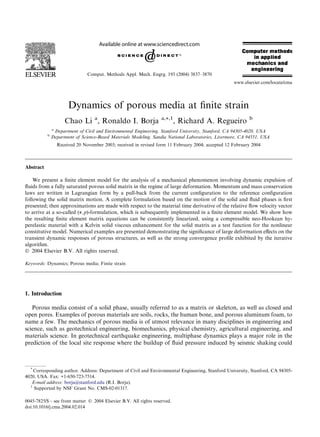
![3838
C. Li et al. / Comput. Methods Appl. Mech. Engrg. 193 (2004) 3837–3870
lead to a rapid loss of strength of the saturated soil deposit, a phenomenon commonly referred to in the
literature as liquefaction [1].
In biomechanics, multiphase dynamics is essential to hard and soft tissue growth and remodeling as
cyclic stresses applied to the tissue solid/fluid mixture generate solid deformation, resulting in fluid flow and
mass transport through the tissue solid matrix leading to cell nutrition, breakdown, and regeneration [2–5].
Multiphase dynamics also plays a significant role during head impacts as skull and brain tissues contact and
deform with concomitant fluid flow in and out of the tissues [6]. Although deformation of bone is small
(0.4% strain [7]), a geometrically nonlinear theory is needed in order to account properly for large rotations
and translations experienced during dynamic loading such as head impact and knee bending. The finite
deformation theory is also necessary for modeling contact of hard tissue with soft tissue (e.g., skull with
brain, bone with cartilage, etc.) and resulting fluid flow. With regard to multi-phase continuum formulations in biomechanics, two- and three-field formulations (and more fields when chemical and electrical
effects are included) have been used for simulating deformation of soft, hydrated biological tissues, such as
cartilage and heart muscle, for small strains [8] and finite strains [9–15].
In geomechanics, multiphase finite element formulations of coupled deformation-fluid flow in porous
media abound in the literature, but a majority of them ignore the effects of solid and fluid accelerations [16–
23]. In the absence of inertia terms the coupled problem is of parabolic type, and the so-called (v; p)formulation is complete (where v ¼ solid velocity field and p ¼ fluid pressure). Large deformation
formulations are available for this type of problem [24–28]. For partially saturated media a three-phase
(v; pw ; pa )-approach offers a direct extension of the two-phase formulation [1,29–31] (where pw ¼ pore water
pressure and pa ¼ pore air pressure).
In the presence of inertia terms the coupled problem is of hyperbolic type, and the so-called (v; p)-formulation is no longer complete. Many authors [1,32–37] have shown that for this class of problem it is
necessary to specify not only the motion of the solid phase but also that of the fluid phase to completely
formulate the governing partial differential equations (PDEs). This can be achieved by specifying, for
example, the fluid velocity field vf , or, alternately, the relative flow velocity vector ~ ¼ vf À v, in addition to
v
the solid velocity field v, resulting in so-called (v; vf )- and (v; ~)-formulations, respectively. The Lagrange
v
multipliers method is sometimes used for ease in the solution process, leading to either the (v; vf ; p)- or the
(v; ~; p)-formulation.
v
Whereas the solution techniques for the hyperbolic PDE for porous media have developed rapidly over
the last decade, most deal only with infinitesimal deformations with the exception of a few. Large deformation formulations based on a hypoelastic theory are subject to criticisms that include, among others, the
fact that it assumes negligible elastic deformations and that a unique objective stress rate cannot be possibly
defined [38]. In addition, the hypoelastic formulation does not conveniently accommodate the commonly
used return mapping algorithm in computational plasticity.
In this paper, we revisit the governing hyperbolic PDEs for fully saturated porous media and write them
out in a form that accommodates the effects of finite deformation. The goal of the paper is to present a
framework that can eventually be used to cast finite deformation multiplicative plasticity models. Thus, we
follow the motion of the solid skeleton in a Lagrangian description and write the momentum balance
equations using this description. The mass balance equations may be interpreted to provide volume constraints to the governing PDEs; by following the motion of the solid phase, we then write the mass balance
equations identifying the spatial point as the instantaneous material point now occupied by the solid phase.
It is noted that it would be very difficult and impractical to write the mass balance equation for the fluid
phase Lagrangian point of view since this would require that we identify and follow the motion of the fluid
material point.
For the hyperbolic problem we write the complete governing PDEs in (v; vf )-form. By assuming that the
material time derivative of the relative velocity vector ~ is zero, we arrive at the reduced (v; p)-form, and this
v
is what we then use in the finite element formulation. As noted in [1,32], this approximation is acceptable in](data:image/gif;base64,R0lGODlhAQABAIAAAAAAAP///yH5BAEAAAAALAAAAAABAAEAAAIBRAA7)