it is well a good

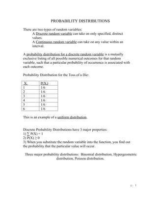
1. PROBABILITY DISTRIBUTIONS
There are two types of random variables:
A Discrete random variable can take on only specified, distinct
values.
A Continuous random variable can take on any value within an
interval.
A probability distribution for a discrete random variable is a mutually
exclusive listing of all possible numerical outcomes for that random
variable, such that a particular probability of occurrence is associated with
each outcome.
Probability Distribution for the Toss of a Die:
Xi P(Xi)
1 1/6
2 1/6
3 1/6
4 1/6
5 1/6
6 1/6
This is an example of a uniform distribution.
Discrete Probability Distributions have 3 major properties:
1) ∑ P(X) = 1
2) P(X) ≥ 0
3) When you substitute the random variable into the function, you find out
the probability that the particular value will occur.
Three major probability distributions: Binomial distribution, Hypergeometric
distribution, Poisson distribution.
p. 1

2. MATHEMATICAL EXPECTATION
A random variable is a variable whose value is determined by chance.
Expected value is a single average value that summarizes a probability
distribution.
E(X) = ∑ XiP(Xi)
If X is a discrete random variable that takes on the value Xi with probability
P(Xi), then the expected value of X – E(X) – is obtained by multiplying each
value that random variable X can assume by its probability P(Xi) and summing
these products. (In other words, it is a weighted average over all possible
outcomes.)
The expected value is normally used as a measure of central tendency for
probability distributions (where ∑P(Xi) = 1). Hence, E(X) = μ.
μ = E(X) = ∑ XiP(Xi)
Example, the probability distribution for the random variable D, the number on
the face of a die after a single toss:
D P(D) D·P(D)
1 1/6 1/6
2 1/6 2/6
3 1/6 3/6
4 1/6 4/6
5 1/6 5/6
6 1/6 6/6
21/6
μ = E(X) = 21/6 = 3.5
The expected value is a single average value that summarizes a probability
distribution. On average, the value you expect from a toss of a die is 3.5. This
is the population mean.
p. 2

3. Variance of a random variable:
σ2 = Var (D) = E[(Di– μ)2] = ∑( Di – μ)2 P(DXi)
σ D = ∑( Di − µ) 2 P ( Di )
2
= (1 − 3.5) 2 ⋅1 / 6
+ ( 2 − 3.5) 2 ⋅1 / 6
+ (3 − 3.5) 2 ⋅1 / 6
+ ( 4 − 3.5) 2 ⋅1 / 6
+ (5 − 3.5) 2 ⋅1 / 6
+ (6 − 3.5) 2 ⋅1 / 6
= 2.9166
σ D =1.71
p. 3

4. Expected Monetary Value
Example:
In the following game, there is an equally likely chance of making $300, $120,
and $0. How much would you be willing to pay to play?
V (Dollar Value) P(V)
$300 1/3
$120 1/3
0 1/3
What is the expected value of this lottery?
E(V) = $140. [$300 (1/3) + $120 (1/3) + $0 (1/3)]. On average, you will make
$140 per game if you play the game for a long, long time.
p. 4

5. Example:
In the particular game, a coin is tossed. If the coin comes up heads, the player
wins $100. If the coin comes up tails, the player loses $50. What is the
expected value of the game?
X (Dollar Value) P(X) X·P(X)
$100 1/2 $50
-$50 1/2 -$25
$25
The expected value of this game is $25. Over the long term, this game is worth
$25 per toss. If you play this game many, many times (say, 1,000 times) on the
average you can expect to make $25 per toss.
Out of, say, 100 tosses, you would expect to win $100 50 times and to lose $50
fifty times. Thus, you will make $2500. This works out to an average winning
of $2500 / 100 = $25.
Don’t pay more than $25 to play.
p. 5

6. Example:
In the following game, there is a one in 4 chance of winning $80; a one in 4
chance of losing $100; and a one-half chance of coming out even. How much
would you be willing to pay to play?
Vi (Dollar Value) P(Vi)
-$100 1/4
0 1/2
+$80 1/4
E(V) = -$5 [-$100 (1/4) + $0 (1/2) + $80 (1/4)]
p. 6

7. Example: a lottery ticket
How much would you be willing to pay for a lottery ticket with a one in 5,000
chance of winning $1 million dollars, and a 4 in 5,000,000 chance of winning
$100,000?
X P(X) X·P(X)
$1,000,00 1 .20
5,000,000
0
$100,000 4 .08
5,000,000
$0 4,999,995 0
5,000,000
$0.28
Answer: Don’t pay more than 28 cents!
p. 7

8. Example:
Would you be willing to pay $9 for a lottery that gives you one chance in a
million of making $5,000,000?
Vi (Dollar Value) P(Vi)
$5,000,000 .000001
$0 .999999
The expected value of the above lottery is $5.00. Mathematically, it does not
make sense to spend $9 for something that has an expected value of only $5.00.
Of course, people do not think this way. Many will spend the $9 or even more
for a chance to make $5 million. Utility theory is used to explain why people
act in this seemingly irrational manner. This is beyond the scope of this course.
p. 8

9. Continuous Probability Distributions
Called a Probability density function. The probability is interpreted as
"area under the curve."
1) The random variable takes on an infinite # of values within a given
interval
2) the probability that X = any particular value is 0. Consequently, we talk
about intervals. The probability is = to the area under the curve.
3) The area under the whole curve = 1.
Some continuous probability distributions: Normal distribution, Standard
Normal (Z) distribution, Student's t distribution, Chi-square ( χ2 )
distribution, F distribution.
p. 9

10. THE NORMAL DISTRIBUTION
The probability density function for the normal distribution:
f(X), the height of the curve, represents the relative frequency at which the
corresponding values occur.
There are 2 parameters: μ for location and σ for shape.
Probabilities are obtained by getting the area under the curve inside of a
particular interval. The area under the curve = the proportion of times under
identical (repeated) conditions that a particular range of values will occur.
The total area under the curve = 1.
Characteristics of the Normal distribution:
1. it is symmetric about the mean μ.
2. mean = median = mode. [“bell-shaped” curve]
3. f(X) decreases as X gets farther and farther away from the mean. It
approaches horizontal axis asymptotically:
-∞<X<+∞
This means that there is always some probability (area) for extreme values.
p. 10

11. Since there are 2 parameters – μ for location and σ for shape. – This means that
there are an infinite number of normal curves – even with the same mean.
Curves A and B are both normal distributions. They have the same mean but
different standard deviations.
μ=30 μ=80 μ=120
σ=5 σ = 10 σ=2
p. 11

12. However, there is only ONE Standard Normal Distribution. This distribution
has a mean of 0 and a standard deviation of 1.
μ=0 σ=1
Any normal distribution can be converted into a standard normal distribution by
transforming the normal random variable into the standard normal r.v.:
X −µ
Z= σ
This is called standardizing the data. It will result in (transformed) data with μ
= 0 and σ = 1.
The Standard Normal Distribution (Z) is tabled:
Please note that you may find different tables for the Z-distribution. The table
we prefer (below), gives you the area from 0 to Z. Some books provide a
slightly different table, one that gives you the area in the tail. If you check the
diagram that is usually shown above the table, you can determine which table
you have. In the table below, the area from 0 to Z is shaded so you know that
you are getting the area from 0 to Z. Also, note that table value can never be
more than .5000. The area from 0 to infinity is .5000.
The Normal Distribution is also referred to as the Gaussian Distribution,
especially in the field of physics. In the social sciences, it is sometimes called
the bell curve because of the way it looks (lucky for us it does not look like a
chicken).
p. 12

13. THE STANDARDIZED NORMAL (Z) DISTRIBUTION
Entry represents area under the standardized normal distribution from the mean to Z
Z .00 .01 .02 .03 .04 .05 .06 .07 .08 .09
0.0 .0000 .0040 .0080 .0120 .0160 .0199 .0239 .0279 .0319 .0359
0.1 .0398 .0438 .0478 .0517 .0557 .0596 .0636 .0675 .0714 .0753
0.2 .0793 .0832 .0871 .0910 .0948 .0987 .1026 .1064 .1103 .1141
0.3 .1179 .1217 .1255 .1293 .1331 .1368 .1406 .1443 .1480 .1517
0.4 .1554 .1591 .1628 .1664 .1700 .1736 .1772 .1808 .1844 .1879
0.5 .1915 .1950 .1985 .2019 .2054 .2088 .2123 .2157 .2190 .2224
0.6 .2257 .2291 .2324 .2357 .2389 .2422 .2454 .2486 .2518 .2549
0.7 .2580 .2612 .2642 .2673 .2704 .2734 .2764 .2794 .2823 .2852
0.8 .2881 .2910 .2939 .2967 .2995 .3023 .3051 .3078 .3106 .3133
0.9 .3159 .3186 .3212 .3238 .3264 .3289 .3315 .3340 .3365 .3389
1.0 .3413 .3438 .3461 .3485 .3508 .3531 .3554 .3577 .3599 .3621
1.1 .3643 .3665 .3686 .3708 .3729 .3749 .3770 .3790 .3810 .3830
1.2 .3849 .3869 .3888 .3907 .3925 .3944 .3962 .3980 .3997 .4015
1.3 .4032 .4049 .4066 .4082 .4099 .4115 .4131 .4147 .4162 .4177
1.4 .4192 .4207 .4222 .4236 .4251 .4265 .4279 .4292 .4306 .4319
1.5 .4332 .4345 .4357 .4370 .4382 .4394 .4406 .4418 .4429 .4441
1.6 .4452 .4463 .4474 .4484 .4495 .4505 .4515 .4525 .4535 .4545
1.7 .4554 .4564 .4573 .4582 .4591 .4599 .4608 .4616 .4625 .4633
1.8 .4641 .4649 .4656 .4664 .4671 .4678 .4686 .4693 .4699 .4706
1.9 .4713 .4719 .4726 .4732 .4738 .4744 .4750 .4756 .4761 .4767
2.0 .4772 .4778 .4783 .4788 .4793 .4798 .4803 .4808 .4812 .4817
2.1 .4821 .4826 .4830 .4834 .4838 .4842 .4846 .4850 .4854 .4857
2.2 .4861 .4864 .4868 .4871 .4875 .4878 .4881 .4884 .4887 .4890
2.3 .4893 .4896 .4898 .4901 .4904 .4906 .4909 .4911 .4913 .4916
2.4 .4918 .4920 .4922 .4925 .4927 .4929 .4931 .4932 .4934 .4936
2.5 .4938 .4940 .4941 .4943 .4945 .4946 .4948 .4949 .4951 .4952
2.6 .4953 .4955 .4956 .4957 .4959 .4960 .4961 .4962 .4963 .4964
2.7 .4965 .4966 .4967 .4968 .4969 .4970 .4971 .4972 .4973 .4974
2.8 .4974 .4975 .4976 .4977 .4977 .4978 .4979 .4979 .4980 .4981
2.9 .4981 .4982 .4982 .4983 .4984 .4984 .4985 .4985 .4986 .4986
3.0 .49865 .49869 .49874 .49878 .49882 .49886 .49889 .49893 .49897 .49900
3.1 .49903 .49906 .49910 .49913 .49916 .49918 .49921 .49924 .49926 .49929
3.2 .49931 .49934 .49936 .49938 .49940 .49942 .49944 .49946 .49948 .49950
3.3 .49952 .49953 .49955 .49957 .49958 .49960 .49961 .49962 .49964 .49965
3.4 .49966 .49968 .49969 .49970 .49971 .49972 .49973 .49974 .49975 .49976
3.5 .49977 .49978 .49978 .49979 .49980 .49981 .49981 .49982 .49983 .49983
3.6 .49984 .49985 .49985 .49986 .49986 .49987 .49987 .49988 .49988 .49989
3.7 .49989 .49990 .49990 .49990 .49991 .49991 .49992 .49992 .49992 .49992
3.8 .49993 .49993 .49993 .49994 .49994 .49994 .49994 .49995 .49995 .49995
3.9 .49995 .49995 .49996 .49996 .49996 .49996 .49996 .49996 .49997 .49997
p. 13

14. REMEMBER THESE PROBABILITIES (percentages):
# s.d. from the mean approx area under the normal curve
±1 .68
±1.645 .90
±1.96 .95
±2 .955
±2.575 .99
±3 .997
p. 14

15. USING THE NORMAL DISTRIBUTION TABLE
Example:
If the weight of males is N.D. with μ=150 and σ=10, what is the probability that
a male will weight between 140 lbs and 155 lbs?
[Important Note:
The probability that X is equal to
any one particular value is zero –
P(X=value) = 0 since the N.D. is
continuous.]
140 −150 − 10
Z= 10 = 10 = -1 s.d. from mean
Area under the curve = .3413 (from Z table)
155 −150 5
Z= 10 = 10 = .5 s.d. from mean
Area under the curve = .1915 (from Z table)
Answer:
.3413
.1915
.5328 
p. 15

16. Example:
If IQ is ND with a mean of 100 and a s.d. of 10, what percentage of the
population will have
(a) IQs ranging from 90 to 110?
(b) IQs ranging from 80 to 120?
(a) Z = (90 – 100) / 10 = -1 area = .3413
Z = (110 – 100) / 10 = +1 area = .3413
.6826 
Answer: 68.26% of the population
(b) Z = (80 – 100) / 10 = -2 area = .4772
Z = (120 – 100) / 10 = +2 area = .4772
.9544 
Answer: 95.44% of the population
Example:
Suppose that the average salary of college graduates is N.D. with μ=$40,000
and σ=$10,000.
(a) What proportion of college graduates will earn less than $24,800?
Z = ($24,800 – $40,000) / $10,000 = −1.52 area = .0643
6.43% of college graduates will earn less than $24,800
(b) What proportion of college graduates will earn more than $53,500?
Z = ($53,500 – $40,000) / $10,000 = +1.35 area = .0885
8.85% of college graduates will earn more than $53,500
p. 16

17. (c) What proportion of college graduates will earn between $45,000 and
$57,000?
Z = ($57,000 – $40,000) / $10,000 = +1.70 area = .4554
Z = ($45,000 – $40,000) / $10,000 = +0.50 area = .1915
Answer: .4554 − .1915 = .2639
(d) Calculate the 80th percentile.
Find the area that corresponds to an area of .3000 from 0 to Z (this means
that there will be .2000 in the tail). A Z value of + 0.84 corresponds to the 80th
percentile.
+.84 = (X − $40,000) / $10,000
X = $40,000 + $8,400 = $48,400. 
[Incidentally, the 20th percentile would be $40,000 − $8,400 = $31,600]
(e) Calculate the 27th percentile.
Find the area that corresponds to an area of .2300 from 0 to Z (this means
that there will be .2700 in the tail). A Z value of − 0.61 corresponds to the 27th
percentile.
− 0.61 = (X − $40,000)/ $10,000
X = $40,000 − $6,100 = $33,900
p. 17

18. Exercise:
The GPA of college students is ND with μ=2.70 and σ=0.25.
(a) What proportion of students have a GPA between 2.40 and 2.50?
(b) Calculate the 97.5th percentile.
[97.5% of college students have a GPA below _______?]
(c) Calculate the 10th Percentile.
[90% of students will have higher GPAs.]
Answers:
The Z-value for the 2.40 GPA converts to -1.20 [ (2.40 – 2.70) / .25 ];
The Z-value for the 2.50 GPA converts to -.80 [ (2.50 – 2.70) / .25 ];
The area from 0 to -1.20 is .3849
The area from 0 to - .80 is .2881
Answer is .3849 - .2881 = .0968 or 9.68% of college students
(b) A z-score of 1.96 is equal to the 97.5th percentile (.5000 + .4750).
Thus, 1.96 = (X – 2.70) / .25
Solve for X. X = .49 + 2.70 = 3.19 Answer = A GPA of 3.19 is the 97.5th
percentile.
(c) A Z score of -1.28 is approximately the 10th percentile.
Find the area that corresponds to an area on the left side (negative) of the
Z-distribution of .4000 from 0 to Z (this means that there will be .1000 in the
tail). A Z value of -1.28 corresponds to the 10th percentile. A Z-score of + 1.28
is approximately the 90th percentile (actually it is .50 + .3997).
Thus, - 1.28 = (X – 2.70) / .25
Solve for X. X = 2.70 - .32 = 2.38 Answer = GPA of 2.38 is the 10th
percentile.
p. 18

19. Exercise:
Chains have a mean breaking strength of 200 lbs, σ=20 lbs.
(a) What proportion of chains will have a breaking strength below 180 lbs?
(b) 99% of chains have breaking points below _________? [99th percentile]
Hint: 50% have breaking points below 200 lbs which is equal to the population
mean. The answer has to be more than 200 lbs. We are on the right side of the
Z distribution.
Answers:
Z = (180 – 200) / 20 = -1.00 The area that is between -1.000 and 0 in the Z
distribution is .3413. We want the left tail below the -1.000. The entire area to
the left of the 0 in the Z-distribution is .5000. Thus,
(a) .5000 - .3413 = .1587 Answer is 15.87%
(b) The value of + 2.33 corresponds to the 99th percentile .5000 + .4901 = .
9901. That is close enough for our purposes.
2.33 = ( X – 200) / 20
X = 246.60 pounds.
p. 19