Lecture notes 02

Chapter 2

Flows under Pressure in Pipes

If the fluid is flowing full in a pipe under pressure with no openings to the atmosphere, it
is called “pressured flow”. The typical example of pressured pipe flows is the water
distribution system of a city.

2.1. Equation of Motion

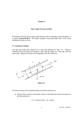
Lets take the steady flow (du/dt=0) in a pipe with diameter D. (Fig. 2.1). Taking a
cylindrical body of liquid with diameter r and with the length Δx in the pipe with the
same center, equation of motion can be applied on the flow direction.

Flow
Δx
α

F2

r
F1
y
D

γπr 2 Δx
x

Figure 2.1.

The forces acting on the cylindrical body on the flow direction are,

a) Pressure force acting to the bottom surface of the body that causes the motion of
the fluid upward is,

→ F1= Pressure force = ( p + Δp )πr 2

1 Prof. Dr. Atıl BULU

b) Pressure force to the top surface of the cylindrical body is,

← F2= Pressure force = pπr 2

c) The body weight component on the flow direction is,

← X = γπr 2 Δx sin α

d) The resultant frictional (shearing) force that acts on the side of the cylindrical
surface due to the viscosity of the fluid is,

← Shearing force = τ 2πrΔx

The equation of motion on the flow direction can be written as,

( p + Δp )πr 2 − pπr 2 − γπr 2 Δx sin α − τ 2πrΔx = Mass × Acceleration (2.1)

The velocity will not change on the flow direction since the pipe diameter is kept
constant and also the flow is a steady flow. The acceleration of the flow body will be
zero, Equ. (2.1) will take the form of,

Δpr 2 − γr 2 Δx sin α − 2τrΔx = 0

1 ⎛ Δp ⎞
τ= ⎜ − γ sin α ⎟r (2.2)
2 ⎝ Δx ⎠

The frictional stress on the wall of the pipe τ0 with r = D/2,

1 ⎛ Δp ⎞D
τ0 = ⎜ − γ sin α ⎟ (2.3)
2 ⎝ Δx ⎠2

We get the variation of shearing stress perpendicular the flow direction from Equs.
(2.2) and (2.3) as,


r
τ =τ0 (2.4)
D2

y

D/2 r

y

τ0 τ

Fig. 2.2

Since r = D/2 –y,

⎛ y ⎞
τ = τ 0 ⎜1 −
⎜ ⎟ (2.5)
⎝ D 2⎟
⎠

The variation of shearing stress from the wall to the center of the pipe is linear as can
be seen from Equ. (2.5).

2.2. Laminar Flow (Hagen-Poiseuille Equation)

Shearing stress in a laminar flow is defined by Newton’s Law of Viscosity as,

du
τ =μ (2.6)
dy

Where μ = (Dynamic) Viscosity and du/dy is velocity gradient in the normal direction
to the flow. Using Equs. (2.5) and (2.6) together,


⎛ y ⎞ du
τ 0 ⎜1 −
⎜ ⎟=μ
⎟
⎝ D 2⎠ dy
τ0 ⎛ y ⎞
du = ⎜1 −
⎜ D 2 ⎟dy
⎟
μ ⎝ ⎠

By taking integral to find the velocity with respect to y,

τ0 ⎛ y ⎞
u=
μ ∫ ⎜1 − D 2 ⎟dy
⎜
⎝
⎟
⎠

τ0 ⎛ y2 ⎞
u= ⎜y−
⎜ ⎟ + cons (2.7)
μ ⎝ D⎟ ⎠

Since at the wall of the pipe (y=0) there will no velocity (u=0), cons=0. If the specific
mass (density) of the fluid is ρ, Friction Velocity is defined as,

τ0
u∗ = (2.8)
ρ

Kinematic viscosity is defined by,

μ μ
υ= →ρ=
ρ υ
τ 0υ τ 0 u ∗2
u∗ =
2
→ =
μ μ υ

The velocity equation for laminar flows is obtained from Equ. (2.7) as,

u∗ ⎛
2
y2 ⎞
u= ⎜y− ⎟ (2.9)
υ ⎜⎝ D⎟ ⎠

Using the geometric relation of the pipe diameter (D) with the distance from the pipe
wall (y) perpendicular to the flow,


D D
r= − y → y = −r
2 2
2 ⎡
⎞ ⎤
2
u D 1 ⎛D
u = ∗ ⎢ − y − ⎜ −r⎟ ⎥
υ ⎢2
⎣ D⎝ 2 ⎠ ⎥⎦

u∗ ⎛ D 2
2
2 ⎞
u= ⎜
⎜ 4 −r ⎟⎟ (2.10)
υD ⎝ ⎠

Equ. (2.10) shows that velocity distribution in a laminar flow is to be a parabolic
curve.

The mean velocity of the flow is,

Q ∫AudA
V= =
A A

Placing velocity equation (Equ. 2.10) gives us the mean velocity for laminar flows as,

2
Du ∗
V= (2.11)
8υ

Since

τ0
u∗ =
2

ρ

And according to the Equ. (2.3),

1 ⎛ Δp ⎞D
τ0 = ⎜ − γ sin α ⎟
2 ⎝ Δx ⎠2


1 ⎛ Δp ⎞D
u∗ =
2
⎜ − γ sin α ⎟
2 ρ ⎝ Δx ⎠2

Placing this to the mean velocity Equation (2.11),

D 2 ⎛ Δp ⎞
V= ⎜ − γ sin α ⎟ (2.11)
32μ ⎝ Δx ⎠

We find the mean velocity equation for laminar flows. This equation shows that
velocity increases as the pressure drop along the flow increases. The discharge of the
flow is,

πD 2
Q = AV = V
4

πD 4 ⎛ Δp ⎞
Q= ⎜ − γ sin α ⎟ (2.12)
128μ ⎝ Δx ⎠

If the pipe is horizontal,

πD 4 Δp
Q= (2.13)
128μ Δx

This is known as Hagen-Poiseuille Equation.

2.3. Turbulent Flow

The flow in a pipe is Laminar in low velocities and Turbulent in high velocities.
Since the velocity on the wall of the pipe flow should be zero, there is a thin layer
with laminar flow on the wall of the pipe. This layer is called Viscous Sub Layer and
the rest part in that cross-section is known as Center Zone. (Fig. 2.3)


δ Viscos Sublayer

y

Center Zone

τ
τ0

Fig. 2.3.

2.3.1. Viscous Sub Layer

Since this layer is thin enough to take the shearing stress as, τ ≈ τ0 and since the flow
is laminar,

du
τ =μ = τ 0 = ρu ∗
2

dy
ρ 2
du = u ∗ dy
μ

By taking the integral,

ρ 2
μ ∫
u= u ∗ dy

ρ 2
u = u ∗ y + cons
μ

Since for y =0 → u = 0, the integration constant will be equal to zero. Substituting
υ=μ/ρ gives,

2
u∗
u= y (2.14)
υ


The variation of velocity with y is linear in the viscous sub layer. The thickness of the
sub layer (δ) has been obtained by laboratory experiments and this empirical equation
has been given,

υ
δ = 11.6 (2.15)
u∗

Example 2.1. The friction velocity u*= 1 cm/sec has been found in a pipe flow with
diameter D = 10 cm and discharge Q = 2 lt/sec. If the kinematic viscosity of the liquid
is υ = 10-2 cm2/sec, calculate the viscous sub layer thickness.

υ
δ = 11.6
u∗
10 − 2
δ = 11.6
1
δ = 0.12cm = 1.2mm

2.3.2 Smooth Pipes

The flow will be turbulent in the center zone and the shearing stress is,

+ (− ρ u ′ v ′)
du
τ =μ (2.16)
dy

The first term of Equ. (2.16) is the result of viscous effect and the second term is the
result of turbulence effect. In turbulent flow the numerical value of Reynolds Stress
(− ρ u ′ v ′) is generally several times greater than that of (μ du dy ) . Therefore, the
viscosity term (μ du dy ) may be neglected in case of turbulent flow.

Shearing stress caused by turbulence effect in Equ. (2.16) can be written in the similar
form as the viscous affect shearing stress as,

du
τ = −ρ u ′v ′ = μ T (2.17)
dy


Here μT is known as turbulence viscosity and defined by,

du
μ T = ρl 2 (2.18)
dy

Here l is the mixing length. It has found by laboratory experiments that l = 0.4y for
τ≈τ0 zone and this 0.4 coefficient is known as Von Karman Coefficient.
Substituting this value to the Equ. (2.18),

du
μ T = 0.16 ρy 2
dy
2
du ⎛ du ⎞
τ 0 = μT = 0.16 ρy 2 ⎜ ⎟
⎜ dy ⎟
dy ⎝ ⎠
2
τ0 ⎛ du ⎞
= u ∗ = 0.16 ρy 2 ⎜ ⎟
2
⎜ dy ⎟
ρ ⎝ ⎠
du
u ∗ = 0.4 y
dy
dy du
= 0.4
y u∗
dy
du = 2.5u ∗
y

Taking the integral of the last equation,

dy
u = 2.5u ∗ ∫
y (2.19)
u = 2.5u ∗ Lny + cons
The velocity on the surface of the viscous sub layer is calculated by using Equs.
(2.14) and (2.15),


2
u∗
u= y
υ
υ
y = δ → δ = 11.6
u∗
u = 11.6u ∗

Substituting this to the Equ. (2.19) will give us the integration constant as,

cons = u − 2.5u ∗ Lny
⎛ υ ⎞
cons = 11.6u ∗ − 2.5u ∗ Ln⎜11.6
⎜ ⎟
⎟
⎝ u∗ ⎠
⎛ υ ⎞
cons = 11.6u ∗ − 2.5u ∗ ⎜ Ln11.6 + Ln
⎜ ⎟
⎟
⎝ u∗ ⎠
υ
cons = 5.5u ∗ − 2.5u ∗ Ln
u∗

Substituting the constant to the Equ. (2.19),

υ
u = 2.5u ∗ Lny + 5.5u ∗ − 2.5u ∗ Ln
u∗

yu ∗
u = 2.5u ∗ Ln + 5.5u ∗
υ
(2.20)
u yu
= 2.5 Ln ∗ + 5.5
u∗ υ

Equ. (2.20) is the velocity equation in turbulent flow in a cross section with respect to
y from the wall of the pipe and valid for the pipes with smooth wall.

The mean velocity at a cross-section is found by the integration of Equ. (2.20) for are
A,


Q
∫ udA
V= = A

A A

⎛ u D ⎞
V = ⎜ 2.5Ln ∗ + 1.75 ⎟u ∗
⎝ 2υ ⎠
(2.21)
V Du ∗
= 2.5 Ln + 1.75
u∗ υ

2.3.3. Definition of Smoothness and Roughness

The uniform roughness size on the wall of the pipe can be e as roughness depth. Most
of the commercial pipes have roughness. The above derived equations are for smooth
pipes. The definition of smoothness and roughness basically depends upon the size of
the roughness relative to the thickness of the viscous sub layer. If the roughnesess are
submerged in the viscous sub layer so the pipe is a smooth one, and resistance and
head loss are entirely unaffected by roughness up to this size.

Pipe Center

Flow

e

Pipe wall

Fig. 2.4

υ
Since the viscous sub layer thickness (δ) is given by, δ = 11.6 pipe roughness size
u∗
e is compared with δ to define if the pipe will be examined as smooth or rough pipe.


υ
a) e < δ = 11.6
u∗

The roughness of the pipe e will be submerged in viscous sub layer. The flow in the
center zone of the pipe can be treated as smooth flow which is given Chap. 2.3.2.
υ
b) e > 70
u∗

The height of the roughness e is higher than viscous sub layer. The flow in the center
zone will be affected by the roughness of the pipe. This flow is named as Wholly
Rough Flow.

υ υ
c) 11.6 < e < 70
u∗ u∗

This flow is named as Transition Flow.

2.3.4. Wholly Rough Pipes

Pipe friction in rough pipes will be governed primarily by the size and pattern of the
roughness. The velocity equation in a cross section will be the same as Equ. (2.19).

u = 2.5u ∗ Lny + cons (2.19)

Since there will be no sub layer left because of the roughness of the pipe, the
integration constant needs to found out. It has been found by laboratory experiments
that,

e
u=o→ y=
30

The integration is calculated as,


e
0 = 2.5u ∗ Ln + const
30
e
const = −2.5u ∗ Ln
30
e
u = 2.5u ∗ Lny − 2.5u ∗ Ln
30

The velocity distribution at a cross section for wholly rough pipes is,

30 y
u = 2.5u ∗ Ln
e
(2.22)
u 30 y
= 2.5Ln
u∗ e

The mean velocity at that cross section is,

⎛ D ⎞
V = u ∗ ⎜ 2.5Ln + 4.73 ⎟
⎝ 2e ⎠
(2.23)
V D
= 2.5Ln + 4.73
u∗ 2e

2.4. Head (Energy) Loss in Pipe Flows

The Bernoulli equation for the fluid motion along the flow direction between points
(1) and (2) is,

p + Δp V12 p V2
z1 + + = z 2 + + 2 + hL (2.24)
γ 2g γ 2g

If the pipe is constant along the flow, V1 = V2,

Δp
hL = − ( z 2 − z1 ) (2.25)
γ


V2
hL
2g
Energy Line

p + Δp H.G.L p
γ γ
Flow

2

Δx

1

Z2
α
Z1
Horizontal Datum

Figure 2.5

If we define energy line (hydraulic) slope J as energy loss for unit weight of fluid
for unit length,

hL
J= (2.26)
Δx

Where Δx is the length of the pipe between points (1) and (2), and using Equs. (2.25)
and (2.26) gives,

Δp z 2 − z 1
J= −
γΔx Δx
(2.27)
Δp
J= − sin α
γΔx


Using Equ. (2.3),

1 ⎛ Δp ⎞D
τ0 = ⎜ − γ sin α ⎟
2 ⎝ Δx ⎠2
γD ⎛ Δp ⎞
τ0 = ⎜ γΔx − sin α ⎟
⎜ ⎟ (2.28)
4 ⎝ ⎠
γD
τ0 = J
4

Using the friction velocity Equ. (2.8),

τ0
u∗ =
ρ
τ 0 = ρu ∗2
γD ρgD
ρu ∗2 = J= J
4 4
2
4u ∗
J= (2.29)
gD

Energy line slope equation has been derived for pipe flows with respect to friction
velocity u*. Mean velocity of the cross section is used in practical applications instead
of frictional velocity. The overall summary of equational relations was given in
Table. (2.1) between frictional velocity u* and the mean velocity V of the cross
section.


Table 2.1. Mathematical Relations between u* and V

Laminar Flow
(Re<2000) 2
Du ∗
V=
8υ

Smooth Flow
Turbulent υ
Flow e < 11.6
u∗ ⎛ Du ∗ ⎞
(Re>2000) V = u ∗ ⎜ 2.5Ln + 1.75 ⎟
⎝ 2υ ⎠

Wholly Rough Flow ⎛ D ⎞
υ V = u ∗ ⎜ 2.5 Ln + 4.73 ⎟
e > 70 ⎝ 2e ⎠
u∗

After calculating the mean velocity V of the cross-section and finding the type of low,
frictional velocity u* is found out from the equations given in Table (2.1). The energy
line (hydraulic) slope J of the flow is calculated by Equ. (2.29). Darcy-Weisbach
equation is used in practical applications which is based on the mean velocity V to
calculate the hydraulic slope J.

f V2
J= (2.30)
D 2g

Where f is named as the friction coefficient or Darcy-Weisbach coefficient. Friction
coefficient f is calculated from table (2.2) depending upon the type of flow where
ρVD VD
Re = = .
μ υ


Table 2.2. Friction Coefficient Equations

Laminar
Flow 64
(Re<200 f =
Re
0)

Smooth Flow
⎛ υ ⎞
⎜ e < 11.6 ⎟
⎜
⎝ u∗ ⎟
⎠ 8 ⎛
= 2.5Ln⎜ Re
f ⎞
⎟ + 1.75
f ⎜ 32 ⎟
Turbulent ⎝ ⎠
Flow
(Re>2000)
Wholly Rough
Flow
⎛ υ ⎞ 8 ⎛D⎞
⎜ e > 70 ⎟
⎜ = 2.5Ln⎜ ⎟ + 4.73
⎝ u∗ ⎟
⎠ f ⎝ 2e ⎠

Transition Flow ⎛
⎜
⎛ υ υ ⎜
⎜11.6 < e < 70 8 ⎛D⎞ 9.2
⎜ = 2.5Ln⎜ ⎟ + 4.73 − 2.5Ln⎜1 +
⎝ u∗ u∗
⎝ 2e ⎠
f ⎜ Re
⎜
⎝ De

The physical explanation of the equations in Table (2.2) gives us the following results.

a) For laminar flows (Re<2000), friction factor f depends only to the Reynolds
number of the flow. f = f (Re )
b) For turbulent flows (Re>2000),

1. For smooth flows, friction factor f is a function of Reynolds number of the flow.
f = f (Re )


2. For trannsition flow f depend on Reyno number (Re) of the flow and relative
ws, ds olds r e r
roughn of the pipe (e/D), f = f (Re, e D)
ness p
3. For wh holly rough flows, f is a fun
h nction of t
the relative roughness (e/D)
e
f = f (e D )

Fric
ction coeffic
cient f is c
calculated fr
from the eq
quations giv in Tabl (2.2). In case of
ven le
turb
bulent flow, the calcul
, lation of f will always be done by trial and error method. A
diag
gram has be prepare to overco
een ed fficulty. It i prepared by Nikura
ome this dif is adse and
show the func
ws ctional relati
ions betwee f and Re, e/D as curv (Figure 2.6)
en , ves. e

Figure 2.6

Sum
mmary

a) Energy loss for uni length of pipe is calc
it culated by D
Darcy-Weisb
bach equati
ion,

f V2
J=
D 2g

For a pipe w length L, the energy loss will be,
with l

A

h L = JL (2.31)

b) The friction coefficient f will either be calculated from the equations given in
Table (2.2) or from the Nikuradse diagram. (Figure 2.6)

2.5. Head Loss for Non-Circular Pipes

Pipes are generally circular. But a general equation can be derived if the cross-section
of the pipe is not circular. Let’s write equation of motion for a non-circular prismatic
pipe with an angle of α to the horizontal datum in a steady flow. Fig. (2.7).

Flow

τ0 α
p
Δx

p+Δp

A

W = γAΔx

P=Wetted
Perimeter

Figure 2.7

( p + Δp )A − pA − τ 0 PΔx − γAΔx sin α = Mass × acceleration

Where P is the wetted perimeter and since the flow is steady, the acceleration of the
flow will be zero. The above equation is then,

ΔpA − τ 0 PΔx − γAΔx sin α = 0
A ⎛ Δp ⎞ (2.32)
τ0 = ⎜ − γ sin α ⎟
P ⎝ Δx ⎠


Where,

A
R= = Hydraulic Radius (2.33)
P

Hydraulic radius is the ratio of wetted area to the wetted perimeter. Substituting this
to the Equ. (2.32),

⎛ Δp ⎞
τ 0 = R⎜ − γ sin α ⎟
⎝ Δx ⎠
⎛ Δp ⎞
τ 0 = γR⎜
⎜ γΔx − sin α ⎟
⎟
⎝ ⎠

Since by Equ. (2.27),

Δp
J= − sin α
γΔx

Shearing stress on the wall of the non-circular pipe,

τ 0 = γRJ (2.34)

For circular pipes,

A πD 2 4 D
R= = = (2.35)
P πD 4
D = 4R

This result is substituted (D=4R) to the all equations derived for the circular pipes to
obtain the equations for non-circular pipes. Table (2.3) is prepared for the equations
as,


Table 2.3.

Circular Pipes Non-Circular pipes
D
τ0 =γ J
4 τ 0 = γRJ

f V2
J= ×
D 2g f V2
J= ×
4R 2 g
f = f (Re, D e )
f = f (Re, 4 R e )
VD
Re =
υ V 4R
Re =
υ

2.6. Hydraulic and Energy Grade Lines

The terms of energy equation have a dimension of length [L ] ; thus we can attach a
useful relationship to them.

p1 V12 p V2
+ + z1 = 2 + 2 + z 2 + h L (2.36)
γ 2g γ 2g

If we were to tap a piezometer tube into the pipe, the liquid in the pipe would rise in
the tube to a height p/γ (pressure head), hence that is the reason for the name
⎛ p V2 ⎞
hydraulic grade line (HGL). The total head ⎜ + ⎜ γ 2g + z ⎟ in the system is greater
⎟
⎝ ⎠
⎛p ⎞ V2
than ⎜ + z ⎟ by an amount
⎜γ ⎟ (velocity head), thus the energy (grade) line (EGL)
⎝ ⎠ 2g
V2
is above the HGL with a distance .
2g

Some hints for drawing hydraulic grade lines and energy lines are as follows.


Figure 2.8
e

1. By definition, the EGL is positio oned above the HGL a amount equal to
an e
the velocity head. Thu if the vel
y us locity is zer as in lak or reserv
ro, ke voir, the
HGL and E EGL will cooincide with the liquid s
h surface. (Figgure 2.8)
2. Head loss f flow in a pipe or c
for channel alw ways means the EGL will lope
w
downward in the direc ction of flow The only exception to this rule occurs
w. y n e
when a pum supplies energy (an pressure to the flo Then an abrupt
mp s nd e) ow. n
rise in the EGL occur from the upstream si to the d
rs ide downstream side of
m
the pump.
3. If energy is abruptly t
s taken out of the flow b for exam
f by, mple, a turbbine, the
EGL and H HGL will dro abruptly as in Fig…
op y ….
4. In a pipe or channel w
r where the pre essure is zer the HGL is coincide with
ro, L ent
the water in the system because p γ = 0 at these point This fact can be
n m ts. t
used to locate the HGL at certain points in th physical system, su as at
L n he l uch
the outlet e of a pipe where the liquid cha
end e, e arges into th atmosphe or at
he ere,
the upstream end, whe the press
m ere sure is zero in the reser
rvoir. (Fig.2
2.8)
5. For steady flow in a pipe tha has unif
y at form physi ical characcteristics
(diameter, rroughness, shape, and so on) alon its length the head loss per
ng h,
unit of leng will be constant; th the slop (Δh L ΔL ) of the E
gth hus pe EGL and
HGL will b constant and parallel along the l
be l length of pi
ipe.
6. If a flow pa
assage chan nges diamete such as i a nozzle or a change in pipe
er, in e
size, the ve
elocity there in will also change; h
e o hence the diistance betwween the
EGL and H HGL will ch hange. Mor reover, the sslope on the EGL will change
e l
because the head per unit length will be la
e h arger in the conduit with the
e w
larger veloccity.
7. If the HGL falls below the pipe, p γ is neg
L w gative, there indicati sub-
eby ing
atmospheri pressure (
ic (Fig.2.8).

A

Figure 2.9

If the pressure head of water is less than the vapor pressure head of the
water ( -97 kPa or -950 cm water head at standard atmospheric pressure),
cavitation will occur. Generally, cavitation in conduits is undesirable. It
increases the head loss and cause structural damage to the pipe from
excessive vibration and pitting of pipe walls. If the pressure at a section in
the pipe decreases to the vapor pressure and stays that low, a large vapor
cavity can form leaving a gap of water vapor with columns of water on
either side of cavity. As the cavity grows in size, the columns of water
move away from each other. Often these of columns of water rejoin later,
and when they do, a very high dynamic pressure (water hammer) can be
generated, possibly rupturing the pipe. Furthermore, if the pipe is thin
walled, such as thin-walled steel pipe, sub-atmospheric pressure can cause
the pipe wall to collapse. Therefore, the design engineer should be
extremely cautious about negative pressure heads in the pipe.


Lecture notes 02

Recommandé

Recommandé

Contenu connexe

Tendances

Tendances (20)

En vedette

En vedette (6)

Similaire à Lecture notes 02

Similaire à Lecture notes 02 (20)

Dernier

Dernier (20)

Lecture notes 02