Time underlies many interesting human behaviors. Thus, the question of how to represent time in connectionist models is very important. One approach is to represent time implicitly by its effects on processing rather than explicitly (as in a spatial representation). The current report develops a proposal along these lines first described by Jordan (1986) which involves the use of recurrent links in order to provide networks with a dynamic memory. In this approach, hidden unit patterns are fed back to themselves; the internal representations which develop thus reflect task demands in the context of prior internal states. A set of simulations is reported which range from relatively simple problems (temporal version of XOR) to discovering syntactic/semantic features for words. The networks are able to learn interesting internal representations which incorporate task demands with memory demands; indeed, in this approach the notion of memory is inextricably bound up with task processing. These representations reveal a rich structure, which allows them to be highly context-dependent while also expressing generalizations across classes of items. These representations suggest a method for representing lexical categories and the type/token distinction.

1. COGNITIVE SCIENCE, 14, 179-211 (1990).
Finding Structure in Time
JEFFREY L. ELMAN
University of California, San Diego
Time underlies many interesting human behaviors. Thus, the question of
how to represent time in connectionist models is very important. One
approach is to represent time implicitly by its effects on processing rather
than explicitly (as in a spatial representation). The current report develops
a proposal along these lines first described by Jordan (1986) which
involves the use of recurrent links in order to provide networks with a
dynamic memory. In this approach, hidden unit patterns are fed back to
themselves; the internal representations which develop thus reflect task
demands in the context of prior internal states. A set of simulations is
reported which range from relatively simple problems (temporal version
of XOR) to discovering syntactic/semantic features for words. The
networks are able to learn interesting internal representations which
incorporate task demands with memory demands; indeed, in this approach
the notion of memory is inextricably bound up with task processing. These
representations reveal a rich structure, which allows them to be highly
context-dependent while also expressing generalizations across classes of
items. These representations suggest a method for representing lexical
categories and the type/token distinction.
___________________________
I would like to thank Jay McClelland, Mike Jordan, Mary Hare, Dave Rumelhart, Mike
Mozer, Steve Poteet, David Zipser, and Mark Dolson for many stimulating discussions. I thank
McClelland, Jordan, and two anonymous reviewers for helpful critical comments on an earlier
draft of this paper.
This work was supported by contract N00014-85-K-0076 from the Office of Naval
Research and contract DAAB-07-87-C-H027 from Army Avionics, Ft. Monmouth. Requests for
reprints should be sent to the Center for Research in Language, C-008; University of California,
San Diego, CA 92093-0108. The author can be reached via electronic mail as
elman@crl.ucsd.edu.
Page 1

2. Introduction
Time is clearly important in cognition. It is inextricably bound up with many behaviors (such as
language) which express themselves as temporal sequences. Indeed, it is difficult to know how
one might deal with such basic problems as goal-directed behavior, planning, or causation
without some way of representing time.
The question of how to represent time might seem to arise as a special problem unique to
parallel processing models, if only because the parallel nature of computation appears to be at
odds with the serial nature of temporal events. However, even within traditional (serial)
frameworks, the representation of serial order and the interaction of a serial input or output with
higher levels of representation presents challenges. For example, in models of motor activity an
important issue is whether the action plan is a literal specification of the output sequence, or
whether the plan represents serial order in a more abstract manner (e.g., Lashley, 1951;
MacNeilage, 1970; Fowler, 1977, 1980; Kelso, Saltzman, & Tuller, 1986; Saltzman & Kelso,
1987; Jordan & Rosenbaum, 1988). Linguistic theoreticians have perhaps tended to be less
concerned with the representation and processing of the temporal aspects to utterances
(assuming, for instance, that all the information in an utterance is somehow made available
simultaneously in a syntactic tree); but the research in natural language parsing suggests that the
problem is not trivially solved (e.g., Frazier & Fodor; 1978; Marcus, 1980). Thus, what is one of
the most elementary facts about much of human activity -that it has temporal extent -is
sometimes ignored and is often problematic.
In parallel distributed processing models, the processing of sequential inputs has been
accomplished in several ways. The most common solution is to attempt to “parallels time” by
giving it a spatial representation. However, there are problems with this approach, and it is
ultimately not a good solution. A better approach would be to represent time implicitly rather
than explicitly. That is, we represent time by the effect it has on processing and not as an
additional dimension of the input.
This paper describes the results of pursuing this approach, with particular emphasis on
problems that are relevant to natural language processing. The approach taken is rather simple,
but the results are sometimes complex and unexpected. Indeed, it seems that the solution to the
problem of time may interact with other problems for connectionist architectures, including the
problem of symbolic representation and how connectionist representations encode structure. The
current approach supports the notion outlined by Van Gelder (1989; see also Smolensky, 1987,
1988; Elman, 1989), that connectionist representations may have a functional compositionality
without being syntactically compositional.
The first section briefly describes some of the problems that arise when time is represented
externally as a spatial dimension. The second section describes the approach used in this work.
The major portion of this report presents the results of applying this new architecture to a diverse
set of problems. These problems range in complexity from a temporal version of the Exclusive-
OR function to the discovery of syntactic/semantic categories in natural language data.
The Problem with Time
One obvious way of dealing with patterns that have a temporal extent is to represent time
explicitly by associating the serial order of the pattern with the dimensionality of the pattern
Page 2

3. vector. The first temporal event is represented by the first element in the pattern vector, the
second temporal event is represented by the second position in the pattern vector; and so on. The
entire pattern vector is processed in parallel by the model. This approach has been used in a
variety of models (e.g., Cottrell, Munro, & Zipser, 1987; Elman & Zipser, 1988; Hanson & Kegl,
1987).
There are several drawbacks to this approach, which basically uses a spatial metaphor for
time. First, it requires that there be some interface with the world which buffers the input so that
it can be presented all at once. It is not clear that biological systems make use of such shift
registers. There are also logical problems; how should a system know when a buffer’s contents
should be examined?
Second, the shift-register imposes a rigid limit on the duration of patterns (since the input
layer must provide for the longest possible pattern), and further suggests that all input vectors be
the same length. These problems are particularly troublesome in domains such as language,
where one would like comparable representations for patterns that are of variable length. This is
as true of the basic units of speech (phonetic segments) as it is of sentences.
Finally, and most seriously, such an approach does not easily distinguish relative temporal
position from absolute temporal position. For example, consider the following two vectors.
[ 0 1 1 1 0 0 0 0 0 ]
[ 0 0 0 1 1 1 0 0 0 ]
These two vectors appear to be instances of the same basic pattern, but displaced in space (or
time, if we give these a temporal interpretation). However, as the geometric interpretation of
these vectors makes clear, the two patterns are in fact quite dissimilar and spatially distant. 1 PDP
models can of course be trained to treat these two patterns as similar. But the similarity is a
consequence of an external teacher and not of the similarity structure of the patterns themselves,
and the desired similarity does not generalize to novel patterns. This shortcoming is serious if
one is interested in patterns in which the relative temporal structure is preserved in the face of
absolute temporal displacements.
What one would like is a representation of time which is richer and which does not have
these problems. In what follows here, a simple architecture is described which has a number of
desirable temporal properties and has yielded interesting results.
Networks with Memory
The spatial representation of time described above treats time as an explicit part of the input.
There is another, very different possibility, which is to allow time to be represented by the effect
it has on processing. This means giving the processing system dynamic properties which are
responsive to temporal sequences. In short, the network must be given memory.
1. The reader may more easily be convinced of this by comparing the locations of the vectors [100], [010], and
[001] in 3-space. Although these patterns might be considered ’temporally displaced’ versions of the same basic pat-
tern, the vectors are very different.
Page 3

4. There are many ways in which this can be
OUTPUT accomplished, and a number of interesting
proposals have appeared in the literature (e.g.
Jordan, 1986; Tank & Hopfield, 1987;
Stornetta, Hogg, & Huberman, 1987;
Watrous & Shastri, 1987; Waibel,
Hanazawa, Hinton, Shikano, & Lang, 1987;
Pineda, 1988; Williams & Zipser, 1988). One
HIDDEN
of the most promising was suggested by
Jordan (1986). Jordan described a network
(shown in Figure 1) containing recurrent
connections which were used to associate a
static pattern (a “Plan”) with a serially
ordered output pattern (a sequence of
“Actions”). The recurrent connections allow
INPUT PLAN the network’s hidden units to see its own
previous output, so that the subsequent
behavior can be shaped by previous
responses. These recurrent connections are
Figure 1. Architecture used by Jordan (1986).
Connections from output to state units are one-for-
what give the network memory.
one, with a fixed weight of 1.0. Not all connections
are shown.
This approach can be modified in
the following way. Suppose a OUTPUT UNITS
network (shown in Figure 2) is
augmented at the input level by
additional units; call these Context
Units. These units are also “hidden” HIDDEN UNITS
in the sense that they interact
exclusively with other nodes
internal to the network, and not the
outside world.
Imagine that there is a INPUT UNITS CONTEXT UNITS
sequential input to be processed,
and some clock which regulates Figure 2. A simple recurrent network in which activations are
presentation of the input to the copied from hidden layer to context layer on a one-for-one
network. Processing would then basis, with fixed weight of 1.0. Dotted lines represent trainable
consist of the following sequence of connections.
events. At time t, the input units
receive the first input in the sequence. Each input might be a single scalar value or a vector,
depending on the nature of the problem. The context units are initially set to 0.5. 2 Both the input
units and context units activate the hidden units; and then the hidden units feed forward to
2. The activation function used here bounds values between 0.0 and 1.0.
Page 4

5. activate the output units. The hidden units also feed back to activate the context units. This
constitutes the forward activation. Depending on the task, there may or may not be a learning
phase in this time cycle. If so, the output is compared with a teacher input and backpropagation
of error (Rumelhart, Hinton, & Williams, 1986) is used to incrementally adjust connection
strengths. Recurrent connections are fixed at 1.0 and are not subject to adjustment. 3 At the next
time step t+1 the above sequence is repeated. This time the context units contain values which
are exactly the hidden unit values at time t. These context units thus provide the network with
memory.
Internal Representation of Time. In feedforward networks employing hidden units and a
learning algorithm, the hidden units develop internal representations for the input patterns which
recode those patterns in a way which enables the network to produce the correct output for a
given input. In the present architecture, the context units remember the previous internal state.
Thus, the hidden units have the task of mapping both an external input and also the previous
internal state to some desired output. Because the patterns on the hidden units are what are saved
as context, the hidden units must accomplish this mapping and at the same time develop
representations which are useful encodings of the temporal properties of the sequential input.
Thus, the internal representations that develop are sensitive to temporal context; the effect of
time is implicit in these internal states. Note, however, that these representations of temporal
context need not be literal. They represent a memory which is highly task and stimulus-
dependent.
Consider now the results of applying this architecture to a number of problems which
involve processing of inputs which are naturally presented in sequence.
Exclusive-OR
The Exclusive-OR (XOR) function has been of interest because it cannot be learned by a simple
two-layer network. Instead, it requires at least three-layers. The XOR is usually presented as a
problem involving 2-bit input vectors (00, 11, 01, 10) yielding 1-bit output vectors (0, 0, 1, 1;
respectively).
This problem can be translated into a temporal domain in several ways. One version
involves constructing a sequence of 1-bit inputs by presenting the 2-bit inputs one bit at a time
(i.e., in two time steps), followed by the 1-bit output; then continuing with another input/output
pair chosen at random. A sample input might be:
1 0 1 0 0 0 0 1 1 1 1 0 1 0 1. . .
Here, the first and second bits are XOR-ed to produce the third; the fourth and fifth are XOR-ed
to give the sixth; and so on. The inputs are concatenated and presented as an unbroken sequence.
In the current version of the XOR problem, the input consisted of a sequence of 3000 bits
constructed in this manner. This input stream was presented to the network shown in Figure 2
(with 1 input unit, 2 hidden units, 1 output unit, and 2 context units), one bit at a time. The task
of the network was, at each point in time, to predict the next bit in the sequence. That is, given
3. A little more detail is in order about the connections between the context units and hidden units. In the network
used here there were one-for-one connections between each hidden unit and each context unit. This implies there are
an equal number of context and hidden units. The upward connections between the context units and the hidden units
were fully distributed, such that each context unit activates all the hidden units.
Page 5

6. the input sequence shown, where one bit is presented at a time, the correct output at
corresponding points in time is shown below.
input: 1 0 1 0 0 0 0 1 1 1 1 0 1 0 1. . .
output: 0 1 0 0 0 0 1 1 1 1 0 1 0 1 ?. . .
Recall that the actual input to the hidden layer consists of the input shown above, as well as
a copy of the hidden unit activations from the previous cycle. The prediction is thus based not
just on input from the world, but also on the network’s previous state (which is continuously
passed back to itself on each cycle).
Notice that, given the temporal structure of this sequence, it is only sometimes possible to
correctly predict the next item. When the network has received the first bit—1 in the example
above—there is a 50% chance that the next bit will be a 1 (or a 0). When the network receives
the second bit (0), however, it should then be possible to predict that the third will be the XOR,
1. When the fourth bit is presented, the fifth is not predictable. But from the fifth bit, the sixth
can be predicted; and so on.
In fact, after 600 passes through a 3,000 bit sequence constructed in this way, the network’s
ability to predict the sequential input closely follows the above schedule. This can be seen by
looking at the sum squared error in the output prediction at successive points in the input. The
error signal provides a useful guide as to when the network recognized a temporal sequence,
because at such moments its outputs exhibit low error. Figure 3 contains a plot of the sum
0.4
0.35
0.3
0.25
Error
0.2
0.15
0.1
0.05
0
0 2 4 6 8 10 12 14
Cycle (m od 12)
Figure 3. Graph of root mean squared error over 12 consecutive inputs in sequential XOR task. Data
points are averaged over 1200 trials.
squared error over 12 time steps (averaged over 1200 cycles). The error drops at those points in
the sequence where a correct prediction is possible; at other points, the error is high. This is an
indication that the network has learned something about the temporal structure of the input, and
is able to use previous context and current input to make predictions about future input. The
network in fact attempts to use the XOR rule at all points in time; this fact is obscured by the
Page 6

7. averaging of error which was done for Figure 3. If one looks at the output activations it is
apparent from the nature of the errors that the network predicts successive inputs to be the XOR
of the previous two. This is guaranteed to be successful every third bit, and will sometimes—-
fortuitously—also result in correct predictions at other times.
It is interesting that the solution to the temporal version of XOR is somewhat different than
the static version of the same problem. In a network with 2 hidden units, one unit is highly
activated when the input sequence is a series of identical elements (all 1s or 0s), whereas the
other unit is highly activated when the input elements alternate. Another way of viewing this is
that the network developed units which were sensitive to high and low-frequency inputs. This is
a different solution than is found with feedforward networks and simultaneously presented
inputs. This suggests that problems may change their nature when cast in a temporal form. It is
not clear that the solution will be easier or more difficult in this form; but it is an important
lesson to realize that the solution may be different.
In this simulation the prediction task has been used in a way which is somewhat analogous
to autoassociation. Autoassociation is a useful technique for discovering the intrinsic structure
possessed by a set of patterns. This occurs because the network must transform the patterns into
more compact representations; it generally does so by exploiting redundancies in the patterns.
Finding these redundancies can be of interest for what they tell us about the similarity structure
of the data set (cf. Cottrell, Munro, & Zipser, 1987; Elman & Zipser, 1988).
In this simulation the goal was to find the temporal structure of the XOR sequence. Simple
autoassociation would not work, since the task of simply reproducing the input at all points in
time is trivially solvable and does not require sensitivity to sequential patterns. The prediction
task is useful because its solution requires that the network be sensitive to temporal structure.
Structure in Letter Sequences
One question which might be asked is whether the memory capacity of the network architecture
employed here is sufficient to detect more complex sequential patterns than the XOR. The XOR
pattern is simple in several respects. It involves single-bit inputs, requires a memory which
extends only one bit back in time, and there are only four different input patterns. More
challenging inputs would require multi-bit inputs of greater temporal extent, and a larger
inventory of possible sequences. Variability in the duration of a pattern might also complicate
the problem.
An input sequence was devised which was intended to provide just these sorts of complications.
The sequence was composed of six different 6-bit binary vectors. Although the vectors were not
derived from real speech, one might think of them as representing speech sounds, with the six
dimensions of the vector corresponding to articulatory features. Table 1 shows the vector for
each of the six letters.
The sequence was formed in two steps. First, the 3 consonants (b, d, g) were combined in
random order to obtain a 1000-letter sequence. Then each consonant was replaced using the
rules
b ¥ ba
d ¥ dii
g ¥ guu
Page 7

8. Table 4: Vector Definitions of Alphabet
Consonant Vowel Interrupted High Back Voiced
b [ 1 0 1 0 0 1 ]
d [ 1 0 1 1 0 1 ]
g [ 1 0 1 0 1 1 ]
a [ 0 1 0 0 1 1 ]
i [ 0 1 0 1 0 1 ]
u [ 0 1 0 1 1 1 ]
Thus, an initial sequence of the form dbgbddg... gave rise to the final sequence
diibaguuubadiidiiguuu... (each letter being represented by one of the above 6-bit vectors). The
sequence was semi-random; consonants occurred randomly, but following a given consonant the
identity and number of following vowels was regular.
The basic network used in the XOR simulation was expanded to provide for the 6-bit input
vectors; there were 6 input units, 20 hidden units, 6 output units, and 20 context units.
The training regimen involved presenting each 6-bit input vector, one at a time, in sequence.
The task for the network was to predict the next input. (The sequence wrapped around, such that
the first pattern was presented after the last.) The network was trained on 200 passes through the
sequence. It was then tested on another sequence which obeyed the same regularities, but created
from a different initial randomization.
The error signal for part of this testing phase is shown in Figure 4.
1.4
1.2 (d)
1
0.8 (g)
(d)
0.6 (d) (g)
0.4 (b)
(i)
(u)
0.2 (i) (i) (u)
(a) (i)
(a)
(u) (u) (i) (i)
0 (u) (u)
Figure 4. Graph of root mean squared error in letter prediction task. labels indicate the correct output
prediction at each point in time. Error is computed over the entire output vector.
Page 8

9. Target outputs are shown in parenthesis, and the graph plots the corresponding error for each
prediction. It is obvious that the error oscillates markedly; at some points in time, the prediction
is correct (and error is low), while at other points in time the ability to correctly predict is
evidently quite poor. More precisely, error tends to be high when predicting consonants, and low
when predicting the vowels.
Given the nature of the sequence, this behavior is sensible. The consonants were ordered
randomly, but the vowels were not. Once the network has gotten a consonant as input, it can
predict the identity of the following vowel. Indeed, it can do more; it knows how many tokens of
the vowel to expect. At the end of the vowel sequence it has no way to predict the next
consonant. At these points in time, the error is high.
This global error pattern does not tell the whole story, however. Remember that the input
patterns (which are also the patterns the network is trying to predict) are 6-bit vectors. The error
shown in Figure 4 is the sum squared error over all 6-bits. Examine the error on a bit-by-bit
basis; a graph of the error for bits [1] and [4] (over 20 time steps) is shown in Figure 5. There is a
1.4 1.4
1.2 1.2
1 1
0.8 0.8
0.6 0.6
(d)
(d)
0.4 0.4 (b)
(g)
0.2 0.2
(g) (d)
(i) (a) (g)
(u) (u) (d)
0 (a) (d) (i) (i) (u)(u) (b) (a) (g) (u) (u) (i) (i) (d) (i) 0 (i) (i) (u) (u) (u) (a) (u) (u) (u) (i) (i) (i) (i)
Figure 5. (a) Graph of root mean squared error in letter prediction task. Error is computed on bit1 ,
representing the feature CONSONANTAL. (b) Graph of root mean squared error in letter prediction
task. Error is computed on bit 4, representing the feature HIGH.
striking difference in the error patterns. Error on predicting the first bit is consistently lower than
error for the fourth bit, and at all points in time. Why should this be so?
The first bit corresponds to the feature Consonant; the fourth bit corresponds to the feature
High. It happens that while all consonants have the same value for the feature Consonant, they
differ for High. The network has learned which vowels follow which consonants; this is why
error on vowels is low. It has also learned how many vowels follow each consonant. An
interesting corollary is that the network also knows how soon to expect the next consonant. The
network cannot know which consonant, but it can correctly predict that a consonant follows. This
is why the bit patterns for Consonant show low error, and the bit patterns for High show high
error. (It is this behavior which requires the use of context units; a simple feedforward network
could learn the transitional probabilities from one input to the next, but could not learn patterns
that span more than two inputs.)
This simulation demonstrates an interesting point. This input sequence was in some ways
more complex than the XOR input. The serial patterns are longer in duration; they are of variable
length so that a prediction depends on a variable mount of temporal context; and each input
Page 9

10. consists of a 6-bit rather than a 1-bit vector. One might have reasonably thought that the more
extended sequential dependencies of these patterns would exceed the temporal processing
capacity of the network. But almost the opposite is true. The fact that there are subregularities (at
the level of individual bit patterns) enables the network to make partial predictions even in cases
where the complete prediction is not possible. All of this is dependent on the fact that the input is
structured, of course. The lesson seems to be that more extended sequential dependencies may
not necessarily be more difficult to learn. If the dependencies are structured, that structure may
make learning easier and not harder.
Discovering the notion “word”
It is taken for granted that learning a language involves (among many other things) learning the
sounds of that language, as well as the morphemes and words. Many theories of acquisition
depend crucially on such primitive types as word, or morpheme, or more abstract categories as
noun, verb, or phrase (e.g., Berwick & Weinberg, 1984; Pinker, 1984). It is rarely asked how it is
that a language learner knows to begin with that these entities exist. These notions are often
assumed to be innate.
Yet in fact, there is considerable debate among linguists and psycholinguists about what are
the representations used in language. Although it is commonplace to speak of basic units such as
“phoneme,” “morpheme,” and “word”, these constructs have no clear and uncontroversial
definition. Moreover, the commitment to such distinct levels of representation leaves a troubling
residue of entities that appear to lie between the levels. For instance, in many languages, there
are sound/meaning correspondences which lie between the phoneme and the morpheme (i.e.,
sound symbolism). Even the concept “word” is not as straightforward as one might think (cf.
Greenberg, 1963; Lehman, 1962). Within English, for instance, there is no consistently definable
distinction between words (e.g., “apple”), compounds (“apple pie”) and phrases (“Library of
Congress” or “man in the street”). Furthermore, languages differ dramatically in what they treat
as words. In polysynthetic languages (e.g., Eskimo) what would be called words more nearly
resemble what the English speaker would call phrases or entire sentences.
Thus, the most fundamental concepts of linguistic analysis have a fluidity which at the very
least suggests an important role for learning; and the exact form of the those concepts remains an
open and important question.
In PDP networks, representational form and representational content often can be learned
simultaneously. Moreover, the representations which result have many of the flexible and graded
characteristics which were noted above. Thus, one can ask whether the notion “word” (or
something which maps on to this concept) could emerge as a consequence of learning the
sequential structure of letter sequences which form words and sentences (but in which word
boundaries are not marked).
Let us thus imagine another version of the previous task, in which the letter sequences form
real words, and the words form sentences. The input will consist of the individual letters (we will
imagine these as analogous to speech sounds, while recognizing that the orthographic input is
vastly simpler than acoustic input would be). The letters will be presented in sequence, one at a
time, with no breaks between the letters in a word, and no breaks between the words of different
sentences.
Such a sequence was created using a sentence generating program and a lexicon of 15
words.4 The program generated 200 sentences of varying length, from 4 to 9 words. The
Page 10

11. sentences were concatenated, forming a stream of 1,270 words. Next, the words were broken into
their letter parts, yielding 4,963 letters. Finally, each letter in each word was converted into a 5-
bit random vector.
The result was a stream of 4,963 separate 5-bit vectors, one for each letter. These vectors
were the input and were presented one at a time. The task at each point in time was to predict the
next letter. A fragment of the input and desired output is shown in Table 2.
Table 6:
Input Output
0110 m 0000 a
0000 a 0111 n
0111 n 1100 y
1100 y 1100 y
1100 y 0010 e
0010 e 0000 a
0000 a 1001 r
1001 r 1001 s
1001 s 0000 a
0000 a 0011 g
0011 g 0111 o
0111 o 0000 a
0000 a 0001 b
0001 b 0111 o
0111 o 1100 y
1100 y 0000 a
0000 a 0111 n
0111 n 0010 d
0010 d 0011 g
0011 g 0100 i
0100 i 1001 r
1001 r 0110 l
0110 l 1100 y
1100 y
4. The program used was a simplified version of the program described in greater detail in the next simulation.
Page 11

12. A network with 5 input units, 20 hidden units, 5 output units, and 20 context units was
trained on 10 complete presentations of the sequence. The error was relatively high at this point;
the sequence was sufficiently random that it would be difficult to obtain very low error without
memorizing the entire sequence (which would have required far more than 10 presentations).
Nonetheless, a graph of error over time reveals an interesting pattern. A portion of the error
is plotted in Figure 6; each data point is marked with the letter that should be predicted at that
3.5
3 (y)
(a) (s)
(a)
(g) (h)
2.5 (m ) (g)
(a)
(t)
2 (a) (b)
Error
(l) (t) (p) (a) (m )
(e) (b) (i)
(i) (h)
1.5 (l)
(d) (r) (h)
(n) (y)
1 (n) (a) (o) (o)
(r) (l) (v) (y) (e) (a) (a) (p)
(e) (p)
(e)
0.5 (y) (e) (y)
(y) (d) (e) (i)
(d) (l)
0 (s) (y)
Figure 6. (a) Graph of root mean squared error in letter-in-word prediction task.
point in time. Notice that at the onset of each new word, the error is high. As more of the word is
received the error declines, since the sequence is increasingly predictable.
The error thus provides a good clue as to what are recurring sequences in the input, and
these correlate highly with words. The information is not categorical, however. The error reflects
statistics of co-occurrence, and these are graded. Thus, while it is possible to determine, more or
less, what sequences constitute words (those sequences bounded by high error), the criteria for
boundaries are relative. This leads to ambiguities, as in the case of the y in they (see Figure 0); it
could also lead to the misidentification of common sequences that incorporate more than one
word, but which co-occur frequently enough to be treated as a quasi-unit. This is the sort of
behavior observed in children, who at early stages of language acquisition may treat idioms and
other formulaic phrases as fixed lexical items (MacWhinney, 1978).
This simulation should not be taken as a model of word acquisition. While listeners are
clearly able to make predictions based on partial input (Marslen-Wilson & Tyler, 1980;
Grosjean, 1980; Salasoo & Pisoni, 1985), prediction is not the major goal of the language
learner. Furthermore, the co-occurrence of sounds is only part of what identifies a word as such.
The environment in which those sounds are uttered, and the linguistic context are equally critical
in establishing the coherence of the sound sequence and associating it with meaning. This
simulation focuses on only a limited part of the information available to the language learner.
The simulation makes the simple point that there is information in the signal which could serve
Page 12

13. as a cue as to the boundaries of linguistic units which must be learned, and it demonstrates the
ability of simple recurrent networks to extract this information.
Discovering lexical classes from word order
Consider now another problem which arises in the context of word sequences. The order of
words in sentences reflects a number of constraints. In languages such as English (so-called
“fixed word-order” languages), the order is tightly constrained. In many other languages (the
“free word-order” languages), there is greater optionality as to word order (but even here the
order is not free in the sense of random). Syntactic structure, selectional restrictions,
subcategorization, and discourse considerations are among the many factors which join together
to fix the order in which words occur. Thus, the sequential order of words in sentences is neither
simple nor is it determined by a single cause. In addition, it has been argued that generalizations
about word order cannot be accounted for solely in terms of linear order (Chomsky, 1957;
Chomsky, 1965). Rather, there is an abstract structure which underlies the surface strings and it
is this structure which provides a more insightful basis for understanding the constraints on word
order.
While it is undoubtedly true that the surface order of words does not provide the most
insightful basis for generalizations about word order, it is also true that from the point of view of
the listener, the surface order is the only thing visible (or audible). Whatever the abstract
underlying structure be, it is cued by the surface forms and therefore that structure is implicit in
them.
In the previous simulation, we saw that a network was able to learn the temporal structure of
letter sequences. The order of letters in that simulation, however, can be given with a small set of
relatively simple rules.5 The rules for determining word order in English, on the other hand, will
be complex and numerous. Traditional accounts of word order generally invoke symbolic
processing systems to express abstract structural relationships. One might therefore easily
believe that there is a qualitative difference in the nature of the computation required for the last
simulation, and that required to predict the word order of English sentences. Knowledge of word
order might require symbolic representations which are beyond the capacity of (apparently) non-
symbolic PDP systems. Furthermore, while it is true, as pointed out above, that the surface
strings may be cues to abstract structure, considerable innate knowledge may be required in order
to reconstruct the abstract structure from the surface strings. It is therefore an interesting question
to ask whether a network can learn any aspects of that underlying abstract structure.
Simple sentences. As a first step, a somewhat modest experiment was undertaken. A sentence
generator program was used to construct a set of short (two and three-word) utterances. 13
classes of nouns and verbs were chosen; these are listed in Table 3. Examples of each category
are given; it will be noticed that instances of some categories (e.g, VERB-DESTROY) may be
included in others (e.g., VERB-TRAN). There were 29 different lexical items.
5. In the worst case, each word constitutes a rule. More hopefully, networks will learn that recurring orthographic
regularities provide additional and more general constraints (cf. Sejnowski & Rosenberg, 1987).
Page 13

14. Table 3: Categories of lexical items used in sentence simulation
Category Examples
NOUN-HUM man, woman
NOUN-ANIM cat, mouse
NOUN-INANIM book, rock
NOUN-AGRESS dragon, monster
NOUN-FRAG glass, plate
NOUN-FOOD cookie, sandwich
VERB-INTRAN think, sleep
VERB-TRAN see, chase
VERB-AGPA move, break
VERB-PERCEPT smell, see
VERB-DESTROY break, smash
VERB-EA eat
The generator program used these categories and the 15 sentence templates given in Table 4
Table 4: Templates for sentence generator
WORD 1 WORDS WORD 3
NOUN-HUM VERB-EAT NOUN-FOOD
NOUN-HUM VERB-PERCEPT NOUN-INANIM
NOUN-HUM VERB-DESTROY NOUN-FRAG
NOUN-HUM VERB-INTRAN
NOUN-HUM VERB-TRAN NOUN-HUM
NOUN-HUM VERB-AGPAT NOUN-INANIM
NOUN-HUM VERB-AGPAT
NOUN-ANIM VERB-EAT NOUN-FOOD
NOUN-ANIM VERB-TRAN NOUN-ANIM
NOUN-ANIM VERB-AGPAT NOUN-INANIM
NOUN-ANIM VERB-AGPAT
NOUN-INANIM VERB-AGPAT
NOUN-AGRESS VERB-DESTORY NOUN-FRAG
NOUN-AGRESS VERB-EAT NOUN-HUM
NOUN-AGRESS VERB-EAT NOUN-ANIM
NOUN-AGRESS VERB-EAT NOUN-FOOD
to create 10,000 random two- and three-word sentence frames. Each sentence frame was then
Page 14

15. filled in by randomly selecting one of the possible words appropriate to each category. Each
word was replaced by a randomly assigned 31-bit vector in which each word was represented by
a different bit. Whenever the word was present, that bit was flipped on. Two extra bits were
reserved for later simulations. This encoding scheme guaranteed that each vector was orthogonal
to every other vector and reflected nothing about the form class or meaning of the words. Finally,
the 27,354 word vectors in the 10,000 sentences were concatenated, so that an input stream of
27,354 31-bit vectors was created. Each word vector was distinct, but there were no breaks
between successive sentences. A fragment of the input stream is shown in column 1 of Table 5,
with the English gloss for each vector in parentheses. The desired output is given in column 2.
Table 5: Fragment of training sequences for sentence simulation
INPUT OUTPUT
0000000000000000000000000000010 (woman) 0000000000000000000000000010000 (smash)
0000000000000000000000000010000 (smash) 0000000000000000000001000000000 (plate)
0000000000000000000001000000000 (plate) 0000010000000000000000000000000 (cat)
0000010000000000000000000000000 (cat) 0000000000000000000100000000000 (move)
0000000000000000000100000000000 (move) 0000000000000000100000000000000 (man)
0000000000000000100000000000000 (man) 0001000000000000000000000000000 (break)
0001000000000000000000000000000 (break) 0000100000000000000000000000000 (car)
0000100000000000000000000000000 (car) 0100000000000000000000000000000 (boy)
0100000000000000000000000000000 (boy) 0000000000000000000100000000000 (move)
0000000000000000000100000000000 (move) 0000000000001000000000000000000 (girl)
0000000000001000000000000000000 (girl) 0000000000100000000000000000000 (eat)
0000000000100000000000000000000 (eat) 0010000000000000000000000000000 (bread)
0010000000000000000000000000000 (bread) 0000000010000000000000000000000 (dog)
0000000010000000000000000000000 (dog) 0000000000000000000100000000000 (move)
0000000000000000000100000000000 (move) 0000000000000000001000000000000 (mouse)
0000000000000000001000000000000 (mouse) 0000000000000000001000000000000 (mouse)
0000000000000000001000000000000 (mouse) 0000000000000000000100000000000 (move)
0000000000000000000100000000000 (move) 1000000000000000000000000000000 (book)
1000000000000000000000000000000 (book) 0000000000000001000000000000000 (lion
For this simulation a network was used which was similar to that in the first simulation,
except that the input layer and output layers contained 31 nodes each, and the hidden and context
layers contained 150 nodes each.
The task given to the network was to learn to predict the order of successive words. The
training strategy was as follows. The sequence of 27,354 31-bit vectors formed an input
sequence. Each word in the sequence was input, one at a time, in order. The task on each input
cycle was to predict the 31-bit vector corresponding to the next word in the sequence. At the end
of the 27,354 word sequence, the process began again without a break starting with the first
Page 15

16. word. The training continued in this manner until the network had experienced 6 complete passes
through the sequence.
Measuring the performance of the network in this simulation is not straightforward. RMS
error after training dropped to 0.88. When output vectors are as sparse as those used in this
simulation (only 1 out of 31 bits turned on), the network quickly learns to turn all the output
units off, which drops error from the initial random value of ~15.5 to 1.0. In this light, a final
error of 0.88 does not seem impressive.
Recall that the prediction task is non-deterministic. Successors cannot be predicted with
absolute certainty. There is thus a built-in error which is inevitable. Nonetheless, although the
prediction cannot be error-free, it is also true that word order is not random. For any given
sequence of words there are a limited number of possible successors. Under these circumstances,
the network should learn the expected frequency of occurrence of each of the possible successor
words; it should then activate the output nodes proportional to these expected frequencies.
This suggests that rather than testing network performance with the RMS error calculated on
the actual successors, the output should be compared with the expected frequencies of
occurrence of possible successors. These expected latter values can be determined empirically
from the training corpus. Every word in a sentence is compared against all other sentences that
are, up to that point, identical. These constitute the comparison set. The probability of occurrence
for all possible successors is then determined from this set. This yields a vector for each word in
the training set. The vector is of the same dimensionality as the output vector, but rather than
representing a distinct word (by turning on a single bit), it represents the likelihood of each
possible word occurring next (where each bit position is a fractional number equal to the
probability). For testing purposes, this likelihood vector can be used in place of the actual teacher
and a RMS error computed based on the comparison with the network output. (Note that it is
appropriate to use these likelihood vectors only for the testing phase. Training must be done on
actual successors, because the point is to force the network to learn the probabilities.)
When performance is evaluated in this manner, RMS error on the training set is 0.053 (sd:
0.100). One remaining minor problem with this error measure is that whereas the elements in the
likelihood vectors must sum to 1.0 (since they represent probabilities), the activations of the
network need not sum to 1.0. It is conceivable that the network output learns the relative
frequency of occurrence of successor words more readily than it approximates exact
probabilities. In this case the shape of the two vectors might be similar, but their length different.
An alternative measure which normalizes for length differences and captures the degree to which
the shape of the vectors is similar is the cosine of the angle between them. Two vectors might be
parallel (cosine of 1.0) but still yield an RMS error, and in this case we might feel that the
network has extracted the crucial information. The mean cosine of the angle between network
output on training items and likelihood vectors is 0.916 (sd: 0.123). By either measure, RMS or
cosine, the network seems to have learned to approximate the likelihood ratios of potential
successors.
How has this been accomplished? The input representations give no information (such as
form-class) that could be used for prediction. The word vectors are orthogonal to each other.
Whatever generalizations are true of classes of words must be learned from the co-occurrence
statistics, and the composition of those classes must itself be learned.
If indeed the network has extracted such generalizations, as opposed to simply memorizing
the sequence, one might expect to see these patterns emerge in the internal representations which
the network develops in the course of learning the task. These internal representations are
Page 16

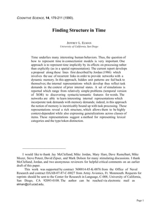
17. captured by the pattern of hidden unit activations which are evoked in response to each word and
its context. (Recall that hidden units are activated by both input units and also context units.
There are no representations of words in isolation.)
The nature of these internal representations was studied in the following way. After the
learning phase of 6 complete passes through the corpus, the connection strengths in the network
were frozen. The input stream was passed through the network one final time, with no learning
taking place. During this testing, the network produced predictions of future inputs on the output
layer. These were ignored. Instead, the hidden unit activations for each word+context input were
saved, resulting in 27,354 150-bit vectors. Each word occurs many times, in different contexts.
As a first approximation of a word’s prototypical or composite representation, all hidden unit
activation patterns produced by a given word (in all its contexts) were averaged to yield a single
150-bit vector for each of the 29 unique words in the input stream. 6 (In the next section we will
see how it is possible to study the internal representations of words in context.) These internal
representations were then subject to a hierarchical clustering analysis. Figure 7 shows the
resulting tree; this tree reflects the similarity structure of the internal representations of these
lexical items. Lexical items which have similar properties are grouped together lower in the tree,
and clusters of similar words which resemble other clusters are connected higher in the tree.
The network has discovered that there are several major categories of words. One large
category corresponds to verbs; another category corresponds to nouns. The verb category is
broken down into groups which require a direct object; which are intransitive; and for which a
direct object is optional. The noun category is broken into major groups for inanimates, and
animates. Animates are divided into human and non-human; the non-human are divided into
large animals and small animals. Inanimates are broken into breakables, edibles, and nouns
which appeared as subjects of agent-less active verbs.
The network has developed internal representations for the input vectors which reflect facts
about the possible sequential ordering of the inputs. The network is not able to predict the precise
order of words, but it recognizes that (in this corpus) there is a class of inputs (viz., verbs) which
typically follow other inputs (viz., nouns). This knowledge of class behavior is quite detailed;
from the fact that there is a class of items which always precedes “chase”, “break”, “smash”, it
infers that the large animals form a class.
Several points should be emphasized. First, the category structure appears to be hierarchical.
Thus, “dragons” are large animals, but also members of the class of [-human, +animate] nouns.
The hierarchical interpretation is achieved through the way in which the spatial relations (of the
representations) are organized. Representations which are near one another in the
representational space form classes, while higher-level categories correspond to larger and more
general regions of this space.
Second, it is also true that the hierarchicality is “soft” and implicit. While some categories
may be qualitatively distinct (i.e., very far from each other in space), there may also be other
6. Tony Plate (personal communication) has pointed out that this technique is dangerous, inasmuch as it may intro-
duce a statistical artifact. The hidden unit activation patterns are highly dependent on preceding inputs. Because the
preceding inputs are not uniformly distributed (they follow precisely the co-occurrence conditions which are appro-
priate for the different categories), this means that the mean hidden unit pattern across all contexts of a specific item
will closely resemble the mean hidden unit pattern for other items in the same category. This could occur even with-
out learning and is a consequence of the averaging of vectors which occurs prior to cluster analysis. Thus the results
of the averaging technique should be verified by clustering individual tokens; tokens should always be closer to other
members of the same type than to tokens of other types.
Page 17

18. smell
move
see think
exist intransitive (always)
sleep
break
smash transitive (sometimes) VERBS
like
chase transitive (always)
eat
mouse
cat
animals
dog
monster
lion ANIMATES
dragon
woman
girl
humans
man
boy
NOUNS
car
book
rock INANIMATES
sandwich
cookie
food
bread
plate
breakables
glass
2.0 1.5 1.0 0.0
Distance
Figure 7. Hierarchical cluster diagram of hidden unit activation vectors in simple sentence prediction task.
labels indicate the inputs which produced the hidden unit vectors; inputs were presented in context, and
the hidden unit vectors averaged across multiple contexts.
Page 18

19. categories which share properties and have less distinct boundaries. Category membership in
some cases may be marginal or unambiguous.
Finally, the content of the categories is not known to the network. The network has no
information available which would “ground” the structural information in the real world. In this
respect, the network has much less information to work with than is available to real language
learners.7 In a more realistic model of acquisition, one might imagine that the utterance provides
one source of information about the nature of lexical categories; the world itself provides another
source. One might model this by embedding the “linguistic” task in an environment; the network
would have the dual task of extracting structural information contained in the utterance, and
extracting structural information about the environment. Lexical meaning would grow out of the
associations of these two types of input.
In this simulation, an important component of meaning is context. The representation of a
word is closely tied up with the sequence in which it is embedded. Indeed, it is incorrect to speak
of the hidden unit patterns as word representations in the conventional sense, since these patterns
also reflect the prior context. This view of word meaning, i.e., its dependence on context, can be
demonstrated in the following way.
Freeze the connections in the network that has just been trained, so that no further learning
occurs. Imagine a novel word, zog, which the network has never seen before (we assign to this
word a bit pattern which is different than those it was trained on). This word will be used in place
of the word man; everywhere that man could occur, zog will occur instead. A new sequence of
10,000 sentences is created, and presented once to the trained network. The hidden unit
activations are saved, and subjected to a hierarchical clustering analysis of the same sort used
with the training data.
The resulting tree is shown in Figure 8. The internal representation for the word zog bears
the same relationship to the other words as did the word man in the original training set. This
new word has been assigned an internal representation which is consistent with what the network
has already learned (no learning occurs in this simulation) and which is consistent with the new
word’s behavior. Another way of looking at this is in certain contexts, the network expects man,
or something very much like it. In just such a way, one can imagine real language learners
making use of the cues provided by word order to make intelligent guesses about the meaning of
novel words.
Although this simulation was not designed to provide a model of context effects in word
recognition, its behavior is consistent with findings that have been described in the experimental
literature. A number of investigators have studied the effects of sentential context on word
recognition. Although some researchers have claimed that lexical access is insensitive to context
(Swinney, 1979), there are other results which suggest that when context is sufficiently strong, it
does indeed selectively facilitate access to related words (Tabossi, Colombo, & Job, 1987).
Furthermore, individual items are typically not very predictable but classes of words are
(Tabossi, 1988; Schwanenflugel & Shoben, 1985). This is precisely the pattern found here, in
which the error in predicting the actual next word in a given context remains high, but the
network is able to predict the approximate likelihood of occurrence of classes of words.
7. Jay McClelland has suggested a humorous--but entirely accurate--metaphor for this task: It is like trying to learn
a language b y listening to the radio.
Page 19

20. smell
move
see think
exist
sleep
break
smash
like
chase
eat
mouse
cat
dog
monster
lion
dragon
woman
girl
boy
ZOG
car
book
rock
sandwich
cookie
bread
plate
glass
2.0 1.5 1.0 0.0 -0.5
Figure 8. Hierarchical clustering diagram of hidden unit activation vectors in simple sentence prediction
task, with the addition of the novel input ZOG.
Types, tokens, and structured representations
There has been considerable discussion about the ways in which PDP networks differ from
traditional computational models. One apparent difference is that traditional models involve
symbolic representations, whereas PDP nets seem to many people to be non- or perhaps sub-
symbolic (Fodor & Pylyshyn, 1988; Smolensky, 1987, 1988). This is a difficult and complex
issue, in part because the definition of symbol is problematic. Symbols do many things, and it
might be more useful to contrast PDP vs. traditional models with regard to the various functions
that symbols can serve.
Both traditional and PDP networks involve representations which are symbolic in the
specific sense that the representations refer to other things. In traditional systems, the symbols
have names such as A, or x, or β. In PDP nets, the internal representations are generally
activation patterns across a set of hidden units. Although both kinds of representations do the
task of referring, there are important differences. Classical symbols typically refer to classes or
categories, whereas in PDP nets the representations may be highly context-dependent. This does
Page 20

21. not mean that the representations do not capture information about category or class (this should
be clear from the previous simulation); it does mean that there is room in the representation
scheme also to pick out individuals.
This property of PDP representations might seem to some to be a serious draw-back. In the
extreme, it suggests that there could be separate representations for the entity John in every
different context in which that entity can occur, leading to an infinite number of Johni. But rather
than being a drawback, I suggest this aspect of PDP networks significantly extends their
representational power. The use of distributed representations, together with the use of context in
representing words (which is a consequence of simple recurrent networks) provides one solution
to a thorny problem -the question of how to represent type/token differences - and sheds insight
on the ways in which distributed representations can represent structure.
In order to justify this claim, let me begin by commenting on the representational richness
provided by the distributed representations developed across the hidden units. In localist
schemes, each node stands for a separate concept. Acquiring new concepts usually requires
adding new nodes. In contrast, the hidden unit patterns in the simulations reported here have
tended to develop distributed representations. In this scheme, concepts are expressed as
activation patterns over a fixed number of nodes. A given node participates in representing
multiple concepts. It is the activation pattern in its entirety that is meaningful. The activation of
an individual node may be uninterpretable in isolation (i.e., it may not even refer to a feature or
micro-feature).
Distributed representations have a number of advantages over localist representations
(although the latter are not without their own benefits). 8 If the units are analog (i.e., capable of
assuming activation states in a continuous range between some minimum and maximum values),
then there is in principle no limit to the number of concepts which can be represented with a
finite set of units. In the simulations here, the hidden unit patterns do double duty. They are
required not only to represent inputs, but to develop representations which will serve as useful
encodings of temporal context which can be used when processing subsequent inputs. Thus, in
theory, analog hidden units would also be capable of providing infinite memory.
Of course, there are many reasons why in practice the memory is bounded, and why the
number of concepts that can be stored is finite. There is limited numeric precision in the
machines on which these simulations are run; the activation function is repetitively applied to the
memory and results in exponential decay; and the training regimen may not be optimal for
exploiting the full capacity of the networks. For instance, many of the simulations reported here
involved the prediction task. This task incorporates feedback on every training cycle. In other
pilot work, it was found that there was poorer performance in tasks in which there was a delay in
injecting error into the network. Still, just what the representational capacity of these simple
recurrent networks is remains an open question (but see Servan-Schreiber, Cleeremans, &
McClelland, 1988).
Having made these preliminary observations, let us now return to the question of the
context-sensitivity of the representations developed in the simulations reported here. Consider
the sentence-processing simulation. It was found that after learning to predict words in sentence
sequences, the network developed representations which reflected aspects of the words’ meaning
as well as their grammatical category. This was apparent in the similarity structure of the internal
representation of each word; this structure was presented graphically as a tree in Figure 7.
8. These advantages are discussed at length in Hinton, McClelland, and Rumelhart (1986).
Page 21

22. In what sense are the representations that have been clustered in Figure 7 context-sensitive?
In fact, they are not; recall that these representations are composites of the hidden unit activation
patterns in response to each word averaged across many different contexts. So the hidden unit
activation pattern used to represent boy, for instance, was really the mean vector of activation
patterns in response to boy as it occurs in many different contexts.
The reason for using the mean vector in the previous analysis was in large part practical. It is
difficult to do a hierarchical clustering of 27,454 patterns, and even more difficult to display the
resulting tree graphically. However, one might want to know whether the patterns displayed in
the tree in Figure 7 are in any way artifactual. Thus, a second analysis was carried out, in which
all 27,454 patterns were clustered. The tree cannot be displayed here, but the numerical results
indicate that the tree would be identical to the tree shown in Figure 7; except that instead of
ending with the terminals that stand for the different lexical items, the branches would continue
with further arborization containing the specific instances of each lexical item in its context. No
instance of any lexical item appears inappropriately in the branch belonging to another.
It would be correct to think of the tree in Figure 7 as showing that the network has
discovered that amongst the sequence of 27,454 inputs, there are 29 types. These types are the
different lexical items shown in that figure. A finer-grained analysis reveals that the network also
distinguishes between the specific occurrences of each lexical item, i.e., the tokens. The internal
representations of the various tokens of a lexical type are very similar. Hence, they all are
gathered under a single branch in the tree. However, the internal representations also make subtle
distinctions between (for example), boy in one context and boy in another. Indeed, as similar as
the representations of the various tokens are, no two tokens of a type are exactly identical.
Even more interesting is that there is a sub-structure of the representations of the various
types of a token. This can be seen by looking at Figure 9, which shows the subtrees
corresponding to the tokens of boy and girl. (Think of these as expansions of the terminal leaves
for boy and girl in Figure 7.) The individual tokens are distinguished by labels which indicate
their original context.
One thing that is apparent is that sub-trees of both types ( boy and girl) are similar to one
another. On closer scrutiny, we see that there is some organization here; (with some exceptions)
tokens of boy which occur in sentence-initial position are clustered together, and tokens of boy in
sentence-final position are clustered together. Furthermore, this same pattern occurs among the
patterns representing girl. Sentence-final words are clustered together on the basis of similarities
in the preceding words. The basis for clustering of sentence-initial inputs is simply that they are
all preceded by what is effectively noise (prior sentences). This is because there are no useful
expectations about the sentence-initial noun (other than that it will be a noun) based on the prior
sentences. On the other hand, one can imagine that if there were some discourse structure
relating sentences to each other, then there might be useful information from one sentence which
would affect the representation of sentence-initial words. For example, such information might
disambiguate (i.e., give referential content to) sentence-initial pronouns.
Once again, it is useful to try to understand these results in geometric terms. The hidden unit
activation patterns pick out points in a high (but fixed) dimensional space. This is the space
available to the network for its internal representations. The network structures that space, in
such a way that important relations between entities is translated into spatial relationships.
Entities which are nouns are located in one region of space and verbs in another. In a similar
manner, different types (here, lexical items) are distinguished from one another by occupying
different regions of space; but also, tokens of a same type are differentiated. The differentiation
Page 22

23. Figure 9. Hierarchical cluster diagram of hidden unit activation vectors in response to some
occurrences of BOY and GIRL. Upper-case labels indicate the actual input; lower-case labels
indicate the context.
is non-random, and the way in which tokens of one type are elaborated is similar to elaboration
of another type. That is, John1 bears the same spatial relationship to John2 as Mary1 bears to
Mary2.
This use of context is appealing, because it provides the basis both for establishing
generalizations about classes of items and also allows for the tagging of individual items by their
context. The result is that we are able to identify types at the same time as tokens. In symbolic
systems, type/token distinctions are often made by indexing or binding operations; the networks
here provide an alternative account of how such distinctions can be made without indexing or
binding.
Conclusions
There are many human behaviors which unfold over time. It would be folly to try to understand
those behaviors without taking into account their temporal nature. The current set of simulations
explores the consequences of attempting to develop an representations of time which are
distributed, task-dependent, and in which time is represented implicitly in the network dynamics.
The approach described here employs a simple architecture but is surprisingly powerful. The
are several points worth highlighting.
• Some problems change their nature when expressed as temporal events. In the first
simulation, a sequential version of the XOR was learned. The solution to this problem
involved detection of state changes, and the development of frequency-sensitive hidden units.
Casting the XOR problem in temporal terms led to a different solution than is typically
obtained in feed-forward (simultaneous input) networks.
Page 23

24. • The time-varying error signal can be used as a clue to temporal structure. Temporal
sequences are not always uniformly structured, nor uniformly predictable. Even when the
network has successfully learned about the structure of a temporal sequence, the error may
vary. The error signal is a good metric of where structure exists; it thus provides a potentially
very useful form of feedback to the system.
• Increasing the sequential dependencies in a task does not necessarily result in worse
performance. In the second simulation, the task was complicated by increasing the
dimensionality of the input vector, by extending the duration of the sequence, and by making
the duration of the sequence variable. Performance remained good, because these
complications were accompanied by redundancy, which provided additional cues for the task.
The network was also able to discover which parts of the complex input were predictable,
making it possible to maximize performance in the face of partial unpredictability.
• The representation of time--and memory--is highly task-dependent. The networks here
depend on internal representations which have available as part of their input their own
previous state. In this way the internal representations inter-mix the demands of the task with
the demands imposed by carrying out that task over time. There is no separate
“representation of time”. There is simply the representation of input patterns in the context of
a given output function; it just happens that those input patterns are sequential. That
representation - and thus the representation of time -varies from task to task. This presents a
somewhat novel view of memory. In this account, memory is neither passive nor a separate
subsystem. One cannot properly speak of a memory for sequences; that memory is
inextricably bound up with the rest of the processing mechanism.
• The representations need not be “flat”, atomistic, or unstructured. The sentence task
demonstrated that sequential inputs may give rise to internal representations which are
hierarchical in nature. The hierarchicality is implicit in the similarity structure of the hidden
unit activations and does not require an a priori architectural commitment to the depth or
form of the hierarchy. Importantly, distributed representations make available a space which
can be richly structured. Categorial relationships as well as type/token distinctions are readily
apparent. Every item may have its own representation, but because the representations are
structured, relations between representations are preserved.
The results described here are preliminary in nature. They are highly suggestive, and often
raise more questions than they answer. These networks are properly thought of as dynamical
systems, and one would like to know more about their properties as such. For instance, the
analyses reported here made frequent use of hierarchical clustering techniques in order to
examine the similarity structure of the internal representations. These representations are
snapshots of the internal states during the course of processing a sequential input. Hierarchical
clustering of these snapshots gives useful information about the ways in which the internal states
of the network at different points in time are similar or dissimilar. But the temporal relationship
between states is lost. One would like to know what the trajectories between states (i.e., the
vectorfield) look like. What sort of attractors develop in these systems? It is a problem, of course,
that the networks studied here are high-dimensional systems and consequently difficult to study
Page 24

25. using traditional techniques. One promising approach which is currently being studied is to carry
out a principal components analysis of the hidden unit activation pattern time series, and then to
construct phase state portraits of the most significant principal components (Elman, 1989).
Another question of interest is what is the memory capacity of such networks. The results
reported here suggest that these networks have considerable representational power; but more
systematic analysis using better defined tasks is clearly desirable. Experiments are currently
underway using sequences generated by finite state automata of various types; these devices are
relatively well-understood, and their memory requirements may be precisely controlled (Servan-
Schreiber, Cleeremans, & McClelland, 1988).
One of the things which feedforward PDP models have shown us is that simple networks are
capable of discovering useful and interesting internal representations of many static tasks. Or put
the other way around: Rich representations are implicit in many tasks. However, many of the
most interesting human behaviors have a serial component. What is exciting about the present
results is that they suggest that the inductive power of the PDP approach can be used to discover
structure and representations in tasks which unfold over time.
Page 25

26. References
Berwick, R.C., & Weinberg, A.S. (1984). The Grammatical Basis of Linguistic Performance.
Cambridge, MA: The MIT Press.
Chomsky, N. Syntactic Structures. The Hague: Moutin, 1957.
Chomsky, N. (1965). Aspects of the theory of syntax. Cambridge, MA: MIT Press.
Cottrell, G.W., Munro, P.W., & Zipser, D. (1987). Image compression by back propagation: A
demonstration of extensional programming. In N.E. Sharkey (Ed.), Advances in cognitive
science (Vol. 2). Chichester, England: Ellis Horwood.
Elman, J.L. (1989). Structured representations and connectionist models. CRL Technical Report
8901. Center for Research in Language, University of California, San Diego.
Elman, J.L., and Zipser, D. (1988). Discovering the hidden structure of speech. Journal of the
Acoustical Society of America, 83, 1615-1626.
Fodor, J., & Pylyshyn, Z. (1988). Connectionism and cognitive architecture: A critical analysis.
In S. Pinker & J. Mehler (Eds.), Connections and Symbols (pp. 3-71). Cambridge, Mass.:
MIT Press.
Fowler, C. (1977). Timing control in speech production. Bloomington, IN: Indiana University
Linguistics Club.
Fowler, C. (1980). Coarticulation and theories of extrinsic timing control. Journal of Phonetics,
88, 113-133.
Frazier, L., & Fodor, J.D. (1978). The sausage machine: A new two-stage parsing model.
Cognition, 66, 291-325.
Greenberg, J.H. (1963). Universals of Language. Cambridge, Ma.: MIT Press.
Grosjean, F. Spoken word recognition processes and the gating paradigm. Perception &
Psychophysics, 1980, 28, 267-283.
Hanson, S.J., & Kegl, J. (1987). Parsnip: A connectionist network that learns natural language
grammar from exposure to natural language sentences. Ninth Annual Conference of the
Cognitive Science Society, Seattle, Washington. Lawrence Erlbaum Associates: Hillsdale,
N.J.
Hinton, G.E., McClelland, J.L., & Rumelhart, D.E. (1986). Distributed representations. In D.E.
Rumelhart & J.L. McClelland (Eds.), Parallel Distributed Processing: Explorations in the
Microstructure of Cognition (Vol. 1) (pp. 77-109). Cambridge, Mass.: MIT Press.
Jordan, M. I. (1986). Serial order: A parallel distributed processing approach. Institute for
Cognitive Science Report 8604. University of California, San Diego.
Jordan, M.I., & Rosenbaum, D.A. (1988). Action. Technical Report 88-26, Department of
Computer Science, University of Massachusetts at Amherst.
Kelso, J.A.S, Saltzman, E., & Tuller, B. (1986). The dynamical theory of speech production:
Data and theory. Journal of Phonetics, 1144, 29-60.
Page 26

27. Lashley, K.S. (1951). The problem of serial order in behavior. In L. A. Jeffress (Ed.), Cerebral
Mechanisms in Behavior. New York: Wiley.
Lehman, W.P. (1962). Historical Linguistics: An Introduction. New York: Holt, Rinehart, and
Winston.
MacNeilage, P.F. (1970). Motor control of serial ordering of speech. Psychological Review, 77,
182-196.
MacWhinney, B. (1978). The acquisition of morphophonology. Monographs of the Society for
Research in Child Development, 43, No. 1.
Marcus, M. (1980). A Theory of Syntactic Recognition for Natural Language. Cambridge, MA:
The MIT Press.
Marslen-Wilson, W., & Tyler, L.K. (1980). The temporal structure of spoken language
understanding. Cognition, 88, 1-71.
Pineda, F.J. (1988). Generalization of backpropagation to recurrent and higher order neural
networks. In Dana Z. Anderson (Ed.), Neural Information Processing Systems. New York:
American Institute of Physics.
Pinker. S. (1984). Language Learnability and Language. Development. Cambridge, Ma.:
Harvard University Press.
Rumelhart, D.E., Hinton, G.E., & Williams, R.J. (1986). Learning internal representations by
error propagation. In D.E. Rumelhart & J.L. McClelland (Eds.), Parallel Distributed
Processing: Explorations in the Microstructure of Cognition (Vol. 1) (pp. 318-362).
Cambridge, MA: MIT Press.
Salasoo, A., & Pisoni, D.B. (1985). Interaction of knowledge sources in spoken word
identification. Journal of Memory and Language, 2244, 210-231.
Saltzman, E., & Kelso, J.A.S. (1987). Skilled actions: A task dynamic approach. Psychological
Review, 9944, 84-106.
Sejnowski, T.J., & Rosenberg, C.R. (1987). Parallel networks that learn to pronounce English
text. Complex Systems, 11, 145-168.
Servan-Schreiber, D., Cleeremans, A., & McClelland, J.L. (1988). Encoding sequential structure
in simple recurrent networks. CMU Technical Report CMU-CS-88-183. Computer Science
Department, Carnegie-Mellon University.
Smolensky, P. (1987). On variable binding and the representation of symbolic structures in
connectionist systems. Technical Report CU-CS-355-87, Department of Computer Science,
University of Colorado.
Smolensky, P. (1988). On the proper treatment of connectionism. The Behavioral and Brain
Sciences, 1111.
Stornetta, W.S., Hogg, T., and Huberman, B.A. (1987). A dynamical approach to temporal
pattern processing. Proceedings of the IEEE Conference on Neural Information Processing
Systems, Denver, Co.
Page 27

28. Tabossi, P. (1988). Effects of context on the immediate interpretation of unambiguous nouns.
Journal of Experimental Psychology: Learning, Memory, and Cognition, 14, 153-162.
Tabossi, P., Colombo, L., & Job, R. (1987). Accessing lexical ambiguity: Effects of context and
dominance. Psychological Research, 49, 161-167.
Tank, D.W., and Hopfield, J.J. (1987). Neural computation by concentrating information in time.
Proceedings of the IEEE International Conference on Neural Networks, San Diego, June
1987.
Waibel, A., Hanazawa, T., Hinton, G., Shikano, K., and Lang, K. (1987). Phoneme recognition
using time-delay neural networks. ATR Technical Report TR-I-0006. Japan: ATR
Interpreting Telephony Research Laboratories
Watrous, R.L., and Shastri, L. (1987). Learning phonetic features using connectionist networks:
An experiment in speech recognition. Proceedings of the IEEE International Conference on
Neural Networks, San Diego, June 1987.
Williams, R.J., & Zipser, D. (1988). A learning algorithm for continually running fully recurrent
neural networks. Institute for Cognitive Science Report 8805. University of California, San
Diego.
Page 28