1. Workshop 14
Pipe Whip Analysis
Introduction
This workshop involves the simulation of a pipe-on-pipe impact resulting from the
rupture of a high-pressure line in a power plant. It is assumed that a sudden release of
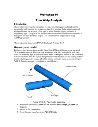
fluid could cause one segment of the pipe to rotate about its support and strike a
neighboring pipe. The goal of the analysis is to determine strain and stress conditions in
both pipes and their deformed shapes. The simulation will be performed using
ABAQUS/Explicit.
This workshop is based on ABAQUS Benchmark Problem 1.3.9.
Geometry and model
Both pipes have a mean diameter of 6.5 in with a .432 in wall thickness and a span of
50 in between supports. The fixed pipe is assumed to be fully restrained at both ends,
while the impacting pipe is allowed to rotate about a fixed pivot located at one of its ends,
with the other end free. We exploit the symmetry of the structure and the loading and thus
model only the geometry on one side of the central symmetry plane, as shown in Figure
W14–1. The pipe geometry is modeled as a shell feature.
Figure W14–1. Pipe model assembly
1. Start a new session of ABAQUS/CAE from the workshops/pipeWhip
directory.
2. Switch to the Part module.
3. From the main menu bar, select PartCreate.
impacting pipe
fixed pipe
axis of rotation
2. 4. In the Create Part dialog box:
A. Name the part pipe-fixed.
B. The pipe will be modeled using shell elements; thus, choose Shell as the base
feature shape, Extrusion as the base feature type, and set the Approximate
size to 20.
C. Review the other defaults and click Continue.
Since the pipe is modeled using a shell feature, the pipe radius must be equal to the mean
pipe radius.
5. Use the Create Isolated Point tool to create points at the coordinates (0.0,
3.25) and (0.0, -3.25).
6. Sketch a circle of radius 3.25 in. as shown in Figure W14–2.
Figure W14–2. Geometry sketch for the fixed pipe
7. Dimension the circle using the radial dimension tool from the toolbox shown as
Figure W14–3.
Figure W14–3. Dimensioning tools
8. Click mouse button 2 to continue; in the Edit Base Extrusion dialog box, enter
25.0 in. as the value of the extrusion depth. (Mouse button 2 is the middle mouse
button on a 3-button mouse; on a 2-button mouse, press both mouse buttons
simultaneously.)
9. From the main menu bar, select PartCopy and copy the part named pipe-
fixed to a new part named pipe-impacting.
W14.2
radial dimension tool
Click on the black
triangle to extend the
toolbox option
3. 10. Switch to the part pipe-impacting by selecting it from the Part pull-down
list in the context bar.
11. From the main menu bar, select FeatureEdit.
12. In the prompt area, click Feature List.
13. In the Feature List dialog box, select Shell-extrude-1 and click OK.
14. In the Edit Feature dialog box select Edit Section Sketch.
15. Delete the circle and sketch a semi-circle with the same radius as shown in
Figure W14–4.
Figure W14–4. Geometry sketch for the impacting pipe
16. Modify the depth of extrusion to be 50.0.
17. In the Edit Feature dialog box, click OK to generate the modified part.
Materials and section
Both pipes are made of steel. A von Mises elastic, perfectly plastic material model is
used, with a yield stress of 45E3 psi.
1. Switch to the Property module.
18. From the main menu bar, select MaterialCreate. Create a material named
Steel with the following properties:
Modulus of elasticity: 30E6 psi
Poisson's ratio: 0.3
Yield Stress: 45.0E3 psi
Density: 7.324E-4 lb-sec2
/in4
19. From the main menu bar, select SectionCreate and create a homogeneous
Shell section named PipeSection with a shell thickness of 0.432 in.
20. Use the analysis default section Poisson ratio of 0.5.
W14.3
4. 21. Select Gauss quadrature for shell section integration with three integration points
through the thickness.
22. From the main menu bar, select AssignSection and assign the shell section to
both parts.
Model assembly
You will now create an instance of each pipe and position them relative to one another.
1. Switch to the Assembly module.
23. From the main menu bar, select InstanceCreate. In the Create Instance
dialog box, select both parts and toggle on Auto-offset from other instances.
24. Modify the position of the impacting part as follows:
A. From the main menu bar, select InstanceTranslate. Select the impacting
pipe as the instance to be translated, and define the translation vector using the
start and end points indicated in Figure W14–5.
Figure W14–5. Translation used to position the impacting pipe
D. From the main menu bar, select InstanceRotate and rotate the impacting
pipe 90 degrees about the axis defined by the two points shown in
Figure W14–6.
W14.4
Start point of translation vector
(center point on bottom edge of
impacting pipe)
End point of translation
vector
5. Figure W14–6. Rotation used to position the impacting pipe
Since ABAQUS/Explicit considers the shell thickness in its contact calculations and does
not permit any initial overclosures, the initial position of the pipes must account for the
shell thickness.
25. Modify the vertical position of the impacting pipe as follows:
· From the main menu bar, select InstanceTranslate. Translate the impacting pipe
a distance of 0.432 in. in the vertical direction. This will eliminate any initial
overclosure between the pipes.
The fixed pivot at the end of the impacting pipe will be modeled using a rigid body
constraint. This constraint will tie the nodes at one end of the impacting pipe with a
reference node that will act as the pivot point.
26. From the main menu bar, select ToolsReference Point and create a reference
point at the location shown in Figure W14–7:
Figure W14–7. Final assembly and reference point
W14.5
end point of rotation axis
start point of rotation axis
6. Analysis step and output requests
Because of the high-speed nature of the event, the simulation is performed using a single
explicit dynamics step.
1. Switch to the Step module.
27. From the main menu bar, select StepCreate to create a Dynamic, Explicit
step with a time period of 0.015 seconds. Accept all defaults for the time
incrementation and other parameters.
28. From the main menu bar, select OutputField Output RequestsEdit
F-Output-1 and review the preselected field output requests. Change the
frequency at which the output is written to 12 equally spaced intervals.
29. Create a geometry set consisting of the reference point. This set will be used to
restrict output of the reaction force history to this region. From the main menu bar,
select ToolsSetCreate. In the Create Set dialog box, name the set RefPt
and click Continue. Select the Ref Pt in the viewport, and click Done.
30. From the main menu bar, select OutputHistory Output Requests
Create and request stored history output to the ODB at 100 equally spaced time
intervals during the analysis containing the following information:
· Reaction forces at the constrained end of the fixed pipe. Use the set RefPt to restrict
the output.
Interactions
You will now define a contact interaction between the two pipes and constrain the pivot
end of the impacting pipe to behave like a rigid body. To facilitate the definition of the
contact interaction and rigid body constraint, the pipes will first be partitioned into
different regions. The partitions will also serve another purpose: they will permit selective
mesh refinement in the regions where contact is expected to take place.
Partitions
The impacting pipe will be divided into three regions of lengths 15, 20, and 15 in.,
respectively. The fixed pipe will be divided into two regions of lengths 18 and 7 in. each.
Partitioning the impacting pipe
1. Switch to the Interaction module.
31. From the main menu bar, select ToolsDatumPlane3 points. Create a
datum plane by selecting the 3 points shown in Figure W14–8.
W14.6
7. Figure W14–8. Points used to define datum plane
32. From the main menu bar, select ToolsPartitionFaceSketch.
33. Select the curved face on the impacting pipe as the face to be partitioned and the
datum plane as the plane on which the partitions will be sketched.
34. Specify the projection distance as Through All and accept the default projection
direction as shown in Figure W14–9.
35. Select the circular edge highlighted in Figure W14–9 when prompted for an edge
that will appear vertical and to the right of the sketch.
Figure W14–9. Sketch projection direction
W14.7
projection
direction
8. 36. Sketch two vertical lines for the partitions as shown in Figure W14–10.
37. Create the partition.
Figure W14–10. Face partition sketch
Partitioning the fixed pipe
1. From the main menu bar, select ToolsPartitionFaceShortest path
between 2 points to partition the fixed pipe using the 2 points highlighted in
Figure W14–11. This partition will later be used for assigning edge seeds.
W14.8
9. Figure W14–11. Face partition using shortest path between 2 points
38. From the main menu bar, select ToolsDatumPlaneOffset from plane.
39. Select the datum plane created earlier as the plane from which to offset.
40. In the prompt area, click Enter Value to choose the method by which to specify
the offset distance. If necessary, flip the direction of the arrow indicating the offset
direction so that it points in the direction shown in Figure W14–12.
41. Specify an offset distance of 7.0 in.
Figure W14–12. Projection direction for fixed pipe partition
W14.9
Select these
two points
offset direction
base datum plane
new datum plane
10. 42. From the main menu bar, select ToolsPartitionFaceUse datum
plane.
43. Select the surface of the fixed pipe as the face to be partitioned and the datum
plane created above as the plane with which to create the partition, as shown in
Figure W14–13.
44. Create the partition.
Figure W14–13. Partition of the fixed pipe
Contact interaction
1. From the main menu bar, select InteractionPropertyCreate.
45. In the Create Interaction Property dialog box, select Contact as the
interaction type and click Continue.
46. In the Edit Contact Property dialog box, select MechanicalTangential
Behavior and choose the Penalty friction formulation. Enter a friction
coefficient of 0.2, and click OK to close the dialog box.
47. From the main menu bar, select InteractionCreate.
48. In the Create Interaction dialog box, choose step-1 as the step in which the
interaction will be created and select the Surface-to-surface contact
(Explicit) type.
For the impacting pipe, the outer surface of its center region will be used for contact; for
the fixed pipe, the outer surface of its shorter region will be used for contact.
49. Define contact between these surfaces as shown in Figure W14–14.
W14.10
Partition the fixed
pipe with this
datum plane
11. Figure W14–14. Surfaces involved in contact
Rigid body constraint
1. From the main menu bar, select ConstraintCreate.
50. In the Create Constraint dialog box, select Rigid body as the constraint type
and click Continue.
51. In the Edit Constraint dialog box, select the region type Tie (nodes) and click
Edit in the right side of the dialog box.
52. Select the edge shown in Figure W14–15 as the tie region for the rigid body.
53. Similarly, select the point in the viewport identified by the label Ref Pt as the
rigid body reference point.
Figure W14–15. Rigid body constraint
master surface slave surface
W14.11
tie region
12. Boundary conditions
The edges located on the symmetry plane must be given appropriate symmetry boundary
conditions. One end of the impacting pipe and both ends of the fixed pipe are fully
restrained.
1. Switch to the Load module.
54. From the main menu bar, select BCCreate.
55. In the Create Boundary Condition dialog box, select Symmetry/
Antisymmetry/Encastre as the boundary condition type and click Continue
to create the boundary conditions shown in Figure W14–16.
· Symmetry boundary conditions: Select the edges shown in Figure W14–16; and in the
Edit Boundary Condition dialog box, choose the ZSYMM (U3=UR1=UR2=0)
boundary condition.
· Fully constrained boundary conditions: Select the edge shown in
Figure W14–16; and in the Edit Boundary Condition dialog box, choose the
ENCASTRE (U1=U2=U3=UR1=UR2=UR3=0) boundary condition.
· Pinned Boundary condition: Select the Ref Pt; and in the Edit Boundary
Condition dialog box, choose the PINNED (U1=U2=U3=0) boundary condition.
Figure W14–16. Boundary conditions
Initial conditions
The impacting pipe is given an initial angular velocity of 75 radians/sec about its
supported (pinned) end.
symmetry: ZSYMM BC
(all edges on this plane)
fully constrained end:
ENCASTRE BC
W14.12
PINNED BC
13. 1. Use ToolsQueryPoint to determine the coordinates of two end points on
the axis of rotation at the pivot end of impacting pipe as shown in
Figure W14–17.
Figure W14–17. Points on axis of rotation
The coordinates will be printed out to the CLI as shown in Figure W14–18.
Figure W14–18. Point coordinates
56. From the main menu bar, select FieldCreate.
57. In the Create Field dialog box, set the step to Initial and accept the default
category and type selections. Click Continue to proceed.
58. Select the impacting pipe as the region to which the initial velocity will be
assigned, and click Done.
59. In the Edit Field dialog box, change the field definition to Rotational only.
Enter a value of 75 for the Angular velocity. Use the coordinates of the first
point indicated in Figure W14–17 to define the first axis point and the coordinates
of the second point indicated in Figure W14–17 to define the second axis point.
Mesh
W14.13
second point
first point
14. The pipes will be meshed with S4R shell elements. A finer mesh density will be used in
the regions of the pipes where impact will is expected to occur.
1. Switch to the Mesh module.
60. From the main menu bar, select MeshElement Type and select the whole
model by clicking the left mouse button and dragging across the viewport.
Examine the various options available in the Element type dialog box, and
accept the default element type S4R.
61. From the main menu bar, select SeedEdge By Number and assign the
number of edge seeds to each edge shown in Figure W14–19.
Figure W14–19. Edge seeds
62. From the main menu bar, select MeshInstance and select both pipes as the
part instances to be meshed. The mesh is shown in Figure W14–20.
W14.14
9
28
9
16
12
9
7
12
15. Figure W14–20. Instance meshes
Analysis
1. Switch to the Job module.
63. From the main menu bar, select JobCreate and create a job named pipe-
whip.
64. Open the Job Manager, and click Submit to submit the job for analysis
65. Monitor the progress of the job by clicking Monitor in the Job Manager.
Visualization
1. Once the analysis completes successfully, click Results in the Job Manager to
switch to the Visualization module.
66. Plot the undeformed and the deformed model shapes. From the main menu bar,
select ToolsColor Code and specify different colors to the two pipe instances,
as shown in Figure W14–21.
W14.15
16. Figure W14–21. Deformed model shape
67. From the main menu bar, select AnimateTime History to animate the
deformation history.
68. Plot the contours for Mises stress and PEEQ on the deformed shape. The contour
plots are shown in Figure W14–22.
Figure W14–22. Contour plots
69. From the main menu bar, select ResultHistory Output to create time history
X–Y plots of the model’s kinetic energy (ALLKE), internal energy (ALLIE), and
dissipated energy (ALLPD).
70. In the History Output dialog box, click Plot to display the curves and click
Dismiss to close the dialog box. The energy plot is shown in Figure W14–23.
W14.16
MISES PEEQ
17. Figure W14–23. Energy histories
Near the end of the simulation, the impacting pipe is beginning to rebound, having
dissipated the majority of its kinetic energy by inelastic deformation in the crushed zone.
71. From the main menu bar, select ToolXY DataManager. In the XY Data
Manager, click Create. In the Create XY Data dialog box, choose ODB
history output and click Continue. Select the three reaction forces
components, and click Save As. Save the components using the default names.
Click Dismiss to close the dialog box.
72. Simultaneously plot the total reaction components (RF1, RF2, RF3) versus time
by selecting the three curves in the XY Data Manager and clicking Plot. The
curves appear in Figure W14–24.
W14.17