Strategic Risk and Performance management by Strategy@Risk Ltd.

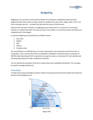
1.
Budgeting
Budgeting is one area that is well suited for Monte Carlo Simulation. Budgeting involves personal
judgments about future values of large number of variables like; sales, prices, wages, down‐ time, error
rates, exchange rates etc. – variables that describes the nature of the business.
Everyone that has been involved in a budgeting process knows that it is an exercise in uncertainty;
however it is seldom described in this way and even more seldom is uncertainty actually calculated as an
integrated part of the budget.
In practice budgeting can be performed on different levels:
1. Cash Flow
2. EBITDA
3. EBIT
4. Profit or
5. Company value.
The most efficient is on EBITDA level, since taxes, depreciation and amortization on the short term is
mostly given. This is also the level where consolidation of daughter companies easiest is achieved. An
EBITDA model describing the firm’s operations can again be used as a subroutine for more detailed and
encompassing analysis thru P&L and Balance simulation.
The aim will then be estimation of the firm’s equity value and is probability distribution. This can again
be used for strategy selection etc.
Forecasting
In today’s fast moving and highly uncertain markets, forecasting have become the single most important
element of the budget process.
Page 1 of 9

2.
Forecasting or predictive analytics can best be described as statistic modeling enabling the prediction of
future events or results, using present and past information and data.
1. Forecasts must integrate both external and internal cost and value drivers of the business
2. Absolute forecast accuracy (i.e. small confidence intervals) is less important than the insight
about how current decisions and likely future events will interact to form the result
3. Detail does not equal accuracy with respect to forecasts
4. The forecast is often less important than the assumptions and variables that underpin it – those
are the things that should be traced to provide advance warning.
5. Never relay on single point or scenario forecasting.
All uncertainty about the market sizes, market shares, cost and prices, interest rates, exchange rates and
taxes etc. – and their correlation will finally end up contributing to the uncertainty in the firm’s budget
forecasts.
The EBITDA model
The EBITDA model have to be detailed enough to capture all important cost and value drivers, but
simple enough to be easy to update with new data and assumptions.
The number of variables and goodness of fit to problem
100
"Inadequate"
80
60
Stress
"Good enough"
40
"Sufficient"
20
0
0 20 40 60 80
Number of variables
Input to the model can come from different sources; any internal reporting system or spread sheet. The
easiest way to communicate with the model is by using Excel1 spread sheet ‐ templates.
Such templates will be pre‐defined in the sense that the information the model needs is on a pre‐
determined place in the workbook. This makes it easy if the budgets for daughter companies is reported
(and consolidated) in a common system (e.g. SAP) and can ‘dump’ onto an excel spread sheet. If the
budgets are communicated directly to head office or the mother company then they can be read
1
The model can also read data written in its own native language: FCS/EPS.
Page 2 of 9

3.
directly by the model. If necessary can S@R “construct” an excel template that includes the cost and
value drivers.
Standalone models and dedicated subroutines
We usually construct our EBITDA models so that they can be used both as a standalone model and as a
subroutine for balance simulation. The model can then be used both for short term budgeting and long‐
term EBITDA forecasting and simulation and for short/long term balance forecasting and simulation.
This means that the same model can be efficiently reused in different contexts.
Rolling budgets and forecast
The EBITDA model can be constructed to give rolling forecast based on updated monthly or quarterly
values, taking into consideration the seasonality of the operations. This will give new forecasts (new
budget) for the remaining of the year and/or the next 12 month. By forecasts we again mean the
probability distributions for the budget variables.
Even if the variables have not changed, the fact that we move towards the end of the year will reduce
the uncertainty of if the end year results and also for the forecast for the next 12 month.
Uncertainty
The most important part of budgeting with Monte Carlo simulation is assessment of the uncertainty in
the budgeted (forecasted) cost and value drivers. This uncertainty is given as the most likely value
(usually the budget figure) and the interval where it is assessed with a high degree of confidence
(approx. 95%) to fall.
We will then use these lower and upper limits (5% and 95%) for sales, prices and other budget items and
the budget values as indicators of the shape of the probability distributions for the individual budget
items. Together they described the range and uncertainty in the EBITDA forecasts.
This gives us the opportunity to simulate (Monte Carlo) a number of possible outcomes – by a large
number of runs of the model, usually 1000 – of net revenue, operating expenses and finally EBITDA. This
again will give us their probability distributions
Most managers and their staff have, based on experience, a good grasp of the range in which the values
of their variables will fall. It is not based on any precise computation but is a reasonable assessment by
knowledgeable persons. Selecting the budget value however is more difficult. Should it be the “mean”
or the “most likely value” or should the manager just delegate fixing of the values to the responsible
departments?
Now we know that the budget values might be biased by a number of reasons – simplest by bonus
schemes etc. – and that budgets based on average assumptions are wrong on average2.
This is therefore where the individual mangers intent and culture will be manifested, and it is here the
greatest learning effect for both the managers and the mother company will be, as under‐budgeting3
2 Savage, Sam L. “The Flaw of Averages”, Harvard Business Review, November 2002, pp. 20-21
3
When the reported most likely value are way below expected value (bonus bias).
Page 3 of 9

4.
and overconfidence4 will stand out as excessive large deviations from the model calculated expected
value (probability weighted average over the interval).
Output
The output from the Monte Carlo simulation will be in the form of graphs that puts all run’s in the
simulation together to form the cumulative distribution for the operating expenses (red line):
100 100
80 80
Probability (%)
60 60
Frequency
40 40
20 20
0 0
870 880 890 900 910 920 930
Operating Expences
In the figure we have computed the frequencies of observed (simulated) values for operating expenses
(blue frequency plot) ‐ the x‐axis gives the operating expenses and the left y‐axis the frequency. By
summing up from left to right we can compute the cumulative probability curve. The s‐shaped curve
(red) gives for every point the probability (on the right y‐axis) for having an operating expenses less than
the corresponding point on the x‐axis. The shape of this curve and its range on the x‐axis gives us the
uncertainty in the forecasts.
A steep curve indicates little uncertainty and a flat curve indicates greater uncertainty. The curve is
calculated from the uncertainties reported in the reporting package or templates.
Large uncertainties in the reported variables will contribute to the overall uncertainty in the EBITDA
forecast and thus to a flatter curve and contrariwise. If the reported uncertainty in sales and prices has a
marked downside and the costs a marked upside the resulting EBITDA distribution might very well have
a portion on the negative side on the x‐axis ‐ that is, with some probability the EBITDA might end up
negative.
In the figure below the lines give the expected EBITDA and the budget value. The expected EBIT can be
found by drawing a horizontal line from the 0.5 (50%) point on the y‐axis to the curve and a vertical line
4
When the reported most likely value are way above expected value (Overconfidence bias, can be cultural or just
lip service).
Page 4 of 9

5.
from this point on the curve to the x‐axis. This point gives us the expected EBITDA value – the point
where it is 50% probability of having a value of EBITDA below and 100%‐50%=50% of having it above.
1
0.8
0.6
Probability
80% 60%
Calculated figure
0.4
0.2
Budget figure
0
40 45 50 55 60 65 70
EBITDA (mill.)
The second set of lines give the budget figure and the probability that it will end up lower than budget.
In this case it is almost a 100% probability that it will be much lower than the management have
expected.
This distributions location on the EBITDA axis (x‐axis) and its shape gives a large amount of information
of what we can expect of possible results and their probability.
The following figure that gives the EBIT distributions for a number of subsidiaries exemplifies this. One
wills most probable never earn money (grey), three is cash cows (blue, green and brown) and the last
(red) can earn a lot of money:
1
0.8
Probability
0.6
0.4
0.2
0
-150 -100 -50 0 50 100 150 200
Budget EBITDA across subsidiaries (mill.)
Page 5 of 9

6.
Budget revisions and follow up
Normally ‐ if something extraordinary does not happen ‐ we would expect both the budget and the
actual EBITDA to fall somewhere in the region of the expected value. We have however to expect some
deviation both from budget and expected value due to the nature of the industry. Having in mind the
possibility of unanticipated events or events “outside” the subsidiary’s budget responsibilities, but
affecting the outcome this implies that:
• Having the actual result deviating from budget is not necessary a sign of bad budgeting
• Having the result close to or on budget is not necessary a sign of good budgeting
However:
• Large deviations between budget and actual result needs looking into – especially if the
deviation to expected value also is large
• Large deviation between budget and expected value can imply either that the limits are set
“wrong” or that the budget EBITDA is not reflecting the downside risk or upside opportunity
expressed by the limits.
1
0.8
Budget
Probability
0.6
Expected
Actual
0.4
0.2
0
-200 -100 0 100 200 300 400 500
EBITDA (mill.)
Another way of looking at the distributions is by the probabilities of having the actual result below
budget that is how far off line the budget ended up. In the graph below, country #1’s budget came out
with a probability of 72% of having the actual result below budget. It turned out that the actual figure
with only 36% probability would have been lower. The length of the bars thus indicates the budget
discrepancies. For country# 2 it is the other way around: the probability of having had a result lower
than the final result is 88% while the budgeted figure had a 63% probability of having been too low. In
this case the market was seriously misjudged.
Page 6 of 9

7.
Probability Range Budget-Actual
The figures give the probability of having the Actual result below Budget.
The other end of the bar indicates the probability of having a result below Actual.
100
80
Accumulated Probability
72
70
64
60 63
40
20
0
ry #1 #2 #3 #4
unt un try unt
ry
un try
Co Co Co Co
In the following we have measured the deviation of the actual result both from the budget values and
from the expected values. In the figures the left axis give the deviation from expected value and the
bottom axis the deviation from budget value.
1. If the deviation for a country falls in the upper right quadrant the deviation are positive for both
budget and expected value – and the country is overachieving.
2. If the deviation falls in the lower left quadrant the deviation are negative for both budget and
expected value – and the country is underachieving.
3. If the deviation falls in the upper left quadrant the deviation are negative for budget and
positive for expected value – and the country is overachieving but has had a to high budget.
With a left skewed EBITDA distribution there should not be any observations in the lower right quadrant
that will only happen when the distribution is skewed to the right – and then there will not be any
observations in the upper left quadrant:
100
Deviation from Expected value by subsidary
80
60
40
20
0
-20
-20 0 20 40
Deviation from Budget by subsidary
Page 7 of 9

8.
As the manager’s gets more experienced in assessing the uncertainty they face, we see that the budget
figures are more in line with the expected values and that the interval’s given is shorter and better
oriented.
1
0.8
2007
2008
Probability 0.6 2009
0.4
0.2
0
0 0.2 0.4 0.6 0.8 1 1.2 1.4
Normalized Budget Uncertainty
If the budget is in line with expected value given the described uncertainty, the upside potential ratio
should be approx. one. A high value should indicate a potential for higher EBITDA and vice versa. Using
this measure we can numerically describe the managements budgeting behavior:
Country Country 1 Country 2 Country 3 Country 4 Country 5 Country 6 Country 7
Upside
2,38 1,58 0,77 0,68 0,58 0,56 0,23
Potential Ratio
Rolling budgets
If the model is set up to give rolling forecasts of the budget EBITDA as new and in this case monthly
data, we will get successive forecast as in the figure below:
Probability distribution for EBITDA
Forecast pr; 1/01, 1/02, 1/03, 1/04, 1/05
1
08
0.6
Probability
0.4
02
0
1000 1500 2000 2500 3000
EBITDA
Page 8 of 9

9.
As data for new month are received, the curve is getting steeper since the uncertainty is reduced. From
the squares on the lines indicating expected value we see that the value is moving slowly to the right
and higher EBITDA values.
We can of course also use this for long term forecasting as in the figure below:
5000
Monthly forecasts of Yearly EBITDA
4000
3000
2000
1000 Forecast pr; 1/01, 1/02, 1/03, 1/04, 1/05
Red lines shows lower 5%, green lines upper 95%
and blue lines the expected values
0
2009 2010 2011 2012 2013 2014 2015 2016
As should now be evident; the EBITDA Monte Carlo model have multiple fields of use and all of them will
increases the managements possibilities of control and foresight‐ giving ample opportunity for prudent
planning for the future.
Page 9 of 9