Oracle Join Methods and 12c Adaptive Plans

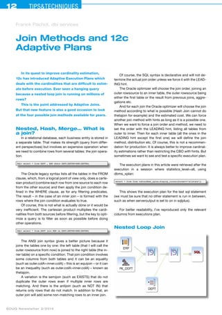
12 Tips&techniques
Franck Pachot, dbi services
Join Methods and 12c
Adaptive Plans
In its quest to improve cardinality estimation,
12c has introduced Adaptive Execution Plans which
deals with the cardinalities that are difficult to estimate
before execution. Ever seen a hanging query
because a nested loop join is running on millions of
rows?
This is the point addressed by Adaptive Joins.
But that new feature is also a good occasion to look
at the four possible join methods available for years.
Nested, Hash, Merge… What is
a join?
In a relational database, each business entity is stored in
a separate table. That makes its strength (query from differ-ent
perspectives) but involves an expensive operation when
we need to combine rows from several tables: the join opera-tion.
SQL> select * from DEPT , EMP where DEPT.DEPTNO=EMP.DEPTNO;
The Oracle legacy syntax lists all the tables in the FROM
clause, which, from a logical point of view only, does a carte-sian
product (combine each row from one source to each row
from the other source) and then apply the join condition de-fined
in the WHERE clause, as for any filtering predicates.
The result – in the case of an inner join – is formed with the
rows where the join condition evaluates to true.
Of course, this is not what is actually done or it would be
very inefficient. The cartesian product multiplies the cardi-nalities
from both sources before filtering, but the key to opti-mize
a query is to filter as soon as possible before doing
other operations.
SQL> select * from DEPT join EMP on DEPT.DEPTNO=EMP.DEPTNO;
The ANSI join syntax gives a better picture because it
joins the tables one by one: the left table (that I will call the
outer rowsource from now) is joined to the right table (the in-ner
table) on a specific condition. That join condition involves
some columns from both tables and it can be an equality
(such as outer.colA=inner.colA) – this is an equijoin – or it can
be an inequality (such as outer.colA>inner.colA) – known as
thetajoin.
A variation is the semijoin (such as EXISTS) that do not
duplicate the outer rows even if multiple inner rows are
matching. And there is the antijoin (such as NOT IN) that
returns only rows that do not match. In addition to that, an
outer join will add some non-matching rows to an inner join.
SOUG Newsletter 2/2014
Of course, the SQL syntax is declarative and will not de-termine
the actual join order unless we force it with the LEAD-ING
hint.
The Oracle optimizer will choose the join order, joining an
outer rowsource to an inner table, the outer rowsource being
either the first table or the result from previous joins, aggre-gations
etc.
And for each join the Oracle optimizer will choose the join
method according to what is possible (Hash Join cannot do
thetajoin for example) and the estimated cost. We can force
another join method with hints as long as it is a possible one.
When we want to force a join order and method, we need to
set the order with the LEADING hint, listing all tables from
outer to inner. Then for each inner table (all the ones in the
LEADING hint except the first one) we will define the join
method, distribution etc. Of course, this is not a recommen-dation
for production. It is always better to improve cardinal-ity
estimations rather than restricting the CBO with hints. But
sometimes we want to see and test a specific execution plan.
The execution plans in this article were retrieved after the
execution in a session where statistics_level=all, using
dbms_xplan:
select * from from table(dbms_xplan.display_cursor(format=>’allstats’))
This shows the execution plan for the last sql statement
(we must be sure that no other statement is run in between,
such as when serveroutput is set to on in sqlplus).
For better readability, I’ve reproduced only the relevant
columns from executions plan.
Nested Loop Join

Tips&ceehinqstu 13
All join methods will read one rowsource and lookup for
matching rows from the other table. What will differ among
the different join methods is the structure used to access ef-ficiently
to that other table. And an efficient access usually
involves sorting or hashing.
■ Nested Loop will use a permanent structure access,
such as an index that is already maintained sorted.
■ Sort Merge join will build a sorted buffer from the inner
table.
■ Hash Join will build a hash table either from the inner
table or the outer rowsource.
■ Merge Join Cartesian will build a buffer from the inner
table, which can be scanned several times.
Nested Loop is special in that it has nothing to do before
starting to iterate over the outer rowsource. Thus, it’s the
most efficient way to return the first row quickly. But because
it does nothing on the inner table before starting the loop, it
requires an efficient way to access to the inner rows: usually
an index access or hash cluster.
Here is the shape of the Nested Loop execution plan in
10g:
EXPLAINED SQL STATEMENT:
------------------------
select * from DEPT join EMP using(deptno) where sal>=3000
------------------------------------------------------------------------
| Id | Operation | Name | Starts | A-Rows | Buffers |
------------------------------------------------------------------------
| 0 | SELECT STATEMENT | | 1 | 3 | 13 |
| 1 | NESTED LOOPS | | 1 | 3 | 13 |
|* 2 | TABLE ACCESS FULL | EMP | 1 | 3 | 8 |
| 3 | TABLE ACCESS BY INDEX ROWID | DEPT | 3 | 3 | 5 |
|* 4 | INDEX UNIQUE SCAN | PK_DEPT | 3 | 3 | 2 |
------------------------------------------------------------------------
Execution Plan 1: Nested Loop Join in 10g
The inner table (EMP) had 3 rows (A-Rows=3) after apply-ing
the ‘sal>=3000’ predicate, and for each of them (Starts=3)
the DEPT has been accessed by a rowid, which is coming
from the index entry. The hints to force that join are:
LEADING(EMP DEPT) for the join order and USE_NL(DEPT)
to use Nested Loop when joining to the inner table DEPT.
Both have to be used, or the CBO may choose another plan.
The big drawback of Nested Loop is the time to access to
the inner table. Here we had to read 5 blocks (2 index
branch+leaf and 2 table blocks) in order to retrieve only 3
rows. If the outer rowsource returns more than a few rows,
then the Nested Loop is probably not an efficient method.
This can be found on the execution plan with the ‘A-Rows’
from outer rowsource that determines the ‘Starts’ to access
to the inner table.
The cost will be higher when the inner table is big (be-cause
of index depth) and when clustering factor is bad (more
logical reads to access the table). It can be much lower when
we don’t need to access to the table at all (index having all
required columns – known as covering index). But a nested
loop that retrieves a lot of rows is always something expen-sive.
Since 9i, prefetching is done when accessing to the inner
table in order to lower the logical reads. A further optimization
has been introduced by 11g with Nested Loop Join Batching.
A first loop retrieves a vector of rowid from the index and
a second loop retrieves the table rows with a batched I/O
(multiblock). It is faster but possible only when we don’t need
the result to be in the same order as the outer rowsource.
Here is the plan in 11g:
--------------------------------------------------------------------------
--------------------------------------------------------------------------
| 1 | NESTED LOOPS | | 1 | 3 | 13 |
| 2 | NESTED LOOPS | | 1 | 3 | 10 |
|* 4 | INDEX UNIQUE SCAN | PK_DEPT | 3 | 3 | 2 |
| 5 | TABLE ACCESS BY INDEX ROWID | DEPT | 3 | 3 | 3 |
--------------------------------------------------------------------------
Execution Plan 2: Nested Loop Join in 11g
The 12c plan is the same except that it shows the follow-ing
note: ‘this is an adaptive plan’. We will see that later.
Nested Loop can be used for all types of joins and is
efficient when we have few rows from outer rowsource that
can be matched to the inner table through an efficient access
path (usually index). It is the fastest way to retrieve the first
rows quickly (pagination except when we need all rows
before in order to sort them).
But when we have large tables to join, Nested Loop do
not scale. The other join method that can do all kind of joins
on large tables is the Sort Merge Join.
Sort Merge Join
Nested Loop can be used for all types of joins but is prob-ably
not optimal for inequalities, because of the cost of the
range scan to access the inner table:
------------------------
select /*+ leading(EMP DEPT) use_nl(DEPT) index(DEPT) */ * from
DEPT join EMP on(EMP.deptno between DEPT.deptno and DEPT.deptno+1 )
where sal>=3000
------------------------------------------------------------------------
------------------------------------------------------------------------
| 1 | NESTED LOOPS | | 1 | 3 | 13 |
| 2 | NESTED LOOPS | | 1 | 3 | 11 |
|* 4 | INDEX RANGE SCAN | PK_DEPT | 3 | 3 | 3 |
| 5 | TABLE ACCESS BY INDEX ROWID| DEPT | 3 | 3 | 2 |
------------------------------------------------------------------------
Execution Plan 3: Nested Loop Join with inequality

14 Tips&techniques
Here I forced the plan to be a nested loop. But it can be
very bad if the range scan returns a lot of rows.
So without hinting, a Sort Merge Sort is chosen by the
CBO for that inequality join:
------------------------
select * from DEPT join EMP
on (EMP.deptno between DEPT.deptno and DEPT.deptno+10 ) where sal>=3000
------------------------------------------------------------------------
| Id | Operation | Name | Starts | A-Rows | Buffers | OMem |
------------------------------------------------------------------------
| 0 | SELECT STATEMENT | | 1 | 5 | 14 | |
| 1 | MERGE JOIN | | 1 | 5 | 14 | |
| 2 | SORT JOIN | | 1 | 3 | 7 | 2048 |
|* 3 | TABLE ACCESS FULL | EMP | 1 | 3 | 7 | |
|* 4 | FILTER | | 3 | 5 | 7 | |
|* 5 | SORT JOIN | | 3 | 5 | 7 | 2048 |
| 6 | TABLE ACCESS FULL | DEPT | 1 | 4 | 7 | |
------------------------------------------------------------------------
Execution Plan 4: Sort Merge Join
The sort merge will use sorted rowsets in order to do the
row matching without additional access. The outer rowsource
is read and because both are sorted in the same way, it is
easy to merge them. It is much quicker than a nested loop,
but has an additional overhead: the rows must be sorted.
The hints to force that plan are LEADING(EMP DEPT) USE_
MERGE(DEPT)
In this example, both rowsources had to be sorted (SORT
JOIN operation). This has an additional cost, and defers the
first row retrieving because the SORT is a blocking operation
(need to be completed before retrieving first result).
But when the outer row source is already ordered, and/or
when the result must be ordered anyway, the Sort merge Join
is an efficient method:
PLAN_TABLE_OUTPUT
------------------------
select * from DEPT join EMP using(deptno) where sal>=3000 order by deptno
-----------------------------------------------------------------------
-----------------------------------------------------------------------
| 1 | MERGE JOIN | | 1 | 3 | 11 | |
|* 2 | TABLE ACCESS BY INDEX
ROWID| EMP | 1 | 3 | 4 | |
| 3 | INDEX FULL SCAN | EMP_DEPTNO |1 | 14 | 2 | |
|* 4 | SORT JOIN | | 3 | 3 | 7 | 2048 |
-----------------------------------------------------------------------
Execution Plan 5: Sort Merge Join without sorting
Here because I have an index on EMP.DEPTNO, which is
ordered, there is no need to sort the outer rowsource. And
there is no need to sort the result of the join because the Sort
Merge Join returns rows in the same order as required by
ORDER BY.
However, even when already sorted, the inner rowsource
must always have a SORT JOIN operation, probably because
only that sort structure (in memory or tempfile) has the ability
to navigate backward when merging. So that join method
always have an overhead before being able to return rows,
even with sorted rowsources as input.
Merge join is very good for large rowsources, when one
rowsource is already ordered, and when we need an ordered
result. For example when joining multiple tables on the same
join predicate, one sort will benefit to all joins. It is the only
efficient join method for inequality joins on large tables.
But when we do an equijoin, hashing is probably a faster
algorithm than sorting.
Hash Join
We have seen that Sort Merge Join is used on large tables
because Nested Loop is not scalable. The problem was that
when we have n rows from the outer rowsource then the
Nested Loop has to access the inner table n times, and each
can involve 2 or 3 blocks through an index access. The best
we can do – in the case of equijoin - is to access through a
Single Table Hash Cluster where each access requires only
one block to read. But Hash clusters as a permanent struc-ture
is difficult to maintain for large tables especially when the
number of rows is difficult to predict. This is why it is not used
as much as indexes.
But in a similar way to the Sort Merge Join that does sort-ing
at each execution instead of accessing an ordered index,
the Hash Join can build a hash table at each execution. The
smallest rowset is used to build that, and then can be probed
efficiently a large number of times.

Tips&ceehinqstu 15
Here is an example of a Hash Join plan:
------------------------
select * from DEPT join EMP using(deptno)
-----------------------------------------------------------------------
-----------------------------------------------------------------------
|* 1 | HASH JOIN | | 1 | 14 | 15 | 1321K |
| 2 | TABLE ACCESS FULL | DEPT | 1 | 4 | 7 |
| 3 | TABLE ACCESS FULL | EMP | 1 | 14 | 8 | |
-----------------------------------------------------------------------
Execution Plan 6: Hash Join
Note that this time DEPT is above EMP. With Hash Join,
inner and outer rowsource can be swapped. The smaller will
be used to build the hash table and is shown above the driv-ing
table.
The plan above, where EMP is still the outer rowsource, is
obtained with the following hints: LEADING(EMP DEPT)
USE_HASH(DEPT) and SWAP_JOIN_INPUTS(DEPT) telling
that DEPT – the inner table – will go above to be the built
(hash) table. We can read those hints as: we have EMP, we
join it to DEPT using a Hash Join and DEPT is the built table.
If we want EMP to be the built table, of course we can
declare the opposite hints: LEADING(DEPT EMP) USE_
HASH(EMP) SWAP_JOIN_INPUTS(EMP). But when we have
more than 2 tables we cannot just change the LEADING
order. Then, we will use the NO_SWAP_JOIN_INPUTS to let
the outer rowsource be the built table.
Merge Join Cartesian
There is another join method that we see rarely. All the join
methods we have seen above have an overhead coming from
the access to the inner table: follow the index tree, sort, hash
etc. What if both tables are so small that we prefer to scan it
as a whole instead of searching an elaborated access path?
We can imagine doing a Nested Loop from a small outer row-source
and FULL SCAN the inner table for each loop. But
there is better: FULL SCAN once, put it in a buffer and then
read the whole buffer for each outer rowsource row.
This is the Merge Join Cartesian:
------------------------
select /*+ leading(DEPT EMP) use_merge_cartesian(EMP) */ * from
DEPT join EMP using(deptno) where sal>3000
------------------------------------------------------------------------
| Id | Operation | Name | Starts | E-Rows | Buffers | OMem |
------------------------------------------------------------------------
| 0 | SELECT STATEMENT | | 1 | | 15 | |
| 1 | MERGE JOIN CARTESIAN | | 1 | 1 | 15 | |
| 3 | BUFFER SORT | | 4 | 1 | 7 | 2048 |
|* 4 | TABLE ACCESS FULL | EMP | 1 | 1 | 7 | |
------------------------------------------------------------------------
Execution Plan 7: Merge join Cartesian
Now the outer rowsource is DEPT, we read 4 rows from it
(‘A-Rows’). For each of them we read the buffer (‘Starts’=4)
but the FULL TABLE SCAN occurred only the first time
(‘Starts’=1). Note that BUFFER SORT – despites its name –
do not do any sorting. It is just buffered. The hints for that are
LEADING(EMP DEPT) USE_MERGE_CARTESIAN(DEPT).
That is a good join method when the inner table is small
but the join cardinality is high (e.g when for each outer row
most of inner rows will match).
12c new feature: Adaptive Join
We have seen at the beginning that in 12c a Nested Loop
was chosen by the optimizer, but mentioning that the plan is
adaptive. Here is the plan with the ‘+adaptive’ format of the
dbms_xplan:
------------------------
------------------------------------------------------------------------
------------------------------------------------------------------------
|- * 1 | HASH JOIN | | 1 | 3 | 12 |
| 2 | NESTED LOOPS | | 1 | 3 | 12 |
| 3 | NESTED LOOPS | | 1 | 3 | 9 |
|- 4 | STATISTICS COLLECTOR | | 1 | 3 | 7 |
| * 5 | TABLE ACCESS FULL | EMP | 1 | 3 | 7 |
| * 6 | INDEX UNIQUE SCAN | PK_DEPT | 3 | 3 | 2 |
| 7 | TABLE ACCESS BY
INDEX ROWID | DEPT | 3 | 3 | 3 |
|- 8 | TABLE ACCESS FULL | DEPT | 0 | 0 | 0 |
------------------------------------------------------------------------
Execution Plan 8: Adaptive Join resolved to Nested Loop
Most of the time, with an equijoin, the choice between
Nested Loop and Hash Join will depend on the size of the
outer rowsource.
If it is overestimated, then we risk doing a Hash join with a
Full Table Scan of the inner table – that is not efficient when
we match only few rows. But underestimating can be worse:
the risk is to do millions of nested loops to access a table.
So 12c defers that choice to the first execution time,
where a STATISTICS COLLECTOR will buffer and count the
rows coming from the outer rowsource until it reaches the
threshold cardinality.

16 Tips&techniques
Then if reached, it will switch to a Hash Join (the outer
rowsource becoming the built table). The threshold is calculated
at parse time where the CBO calculates the cost
for Nested Loop and Hash Join for different cardinalities
(dichotomy until Nested Loop cost is higher than Hash join
cost).
The inflection point can be seen in the optimizer trace
(event 10053). In my example it shows:
Found point of inflection for NLJ vs. HJ: card = 9.30
meaning that execution will switch to Hash Join when
more than 10 rows are returned from EMP.
Here is the execution plan for the same query where the
actual number of rows is 1000 instead of 3
------------------------
------------------------------------------------------------------------
------------------------------------------------------------------------
| * 1 | HASH JOIN | | 1 | 1000 | 14 |
|- 2 | NESTED LOOPS | | 1 | 1000 | 7 |
|- 3 | NESTED LOOPS | | 1 | 1000 | 7 |
|- 4 | STATISTICS COLLECTOR | | 1 | 1000 | 7 |
| * 5 | TABLE ACCESS FULL | EMP | 1 | 1000 | 7 |
|- * 6 | INDEX UNIQUE SCAN | PK_DEPT | 0 | 0 | 0 |
|- 7 | TABLE ACCESS BY
INDEX ROWID | DEPT | 0 | 0 | 0 |
| 8 | TABLE ACCESS FULL | DEPT | 1 | 4 | 7 |
------------------------------------------------------------------------
Execution Plan 9: Adaptive Join resolved to Hash Join
The first 10 rows have been buffered, and then the nested
loop has been discarded in favor of hash join. That inactivates
the 1000 table access by index that would be necessary in
nested loop.
Note that the choice occurs only on the first execution.
Once the first execution has been done, the same plan will be
used by the subsequent executions. We can see than in
V$SQL:
■ IS_RESOLVED_ADAPTIVE_PLAN=N when plan is
adaptive but first execution did not occur yet
■ IS_RESOLVED_ADAPTIVE_PLAN=Y when the choice
has been done – after EXECUTIONS >= 1
So this is a solution when estimation was bad, but not a
solution when data changes. Another 12c feature, Automatic
Reoptimization, is there to adapt for subsequent executions.
Conclusion
Each join method has its use cases where it is efficient:
■ Nested Loop Join is good when we want to retrieve few
rows for which we have a fast access path. This is
typical of OLTP. Proper indexing is the key to good
performance.
■ Hash Join is good when we have large tables, typical
of reporting or BI, especially when the smallest table fits
in memory. But it is available only for equijoins.
■ Merge Join Cartesian should be seen only with small
tables and with a high multiplicity for the join.
■ Sort Merge Join can be seen when the sorting is not
a big overhead, or for thetajoins where hash join is not
possible.
About resources, Nested Loops is more about indexes,
buffer cache (SGA), flash cache and single block reads. Sort
Merge and Hash Joins are more about full table scan, multi-block
reads, direct reads/smartscan and workarea (PGA)
and tempfiles.
The choice among the possible methods depends mainly
on the size of the tables. The estimation can be quite good
for a two table join with accurate object statistics, and/or
dynamic sampling. But after several joins and predicate
filters, the error made by the optimizer may be large, leading
to an inefficient execution plan.
Some cardinality estimations can be more accurate at
execution time. This is why 10g introduced bind variable
peeking, and 11g came with Adaptive Cursor Sharing. And
now 12c goes a step further with Adaptive Plans where a plan
chosen for small rowsource can be adapted when the actual
number of rows is higher than expected. ■
Contact
dbi services
Franck Pachot
E-Mail:
franck.pachot@dbi-services.com

Oracle Join Methods and 12c Adaptive Plans

Recommandé

Recommandé

Contenu connexe

Tendances

Tendances (20)

En vedette

En vedette (20)

Similaire à Oracle Join Methods and 12c Adaptive Plans

Similaire à Oracle Join Methods and 12c Adaptive Plans (20)

Plus de Franck Pachot

Plus de Franck Pachot (7)

Dernier

Dernier (20)

Oracle Join Methods and 12c Adaptive Plans