Grants and Outcomes

HANMING FANG
Yale University
MICHAEL P. KEANE
Yale University

Assessing the Impact of Welfare
Reform on Single Mothers

THE PERSONAL RESPONSIBILITY and Work Opportunity Reconciliation
Act (PRWORA), signed into law in 1996, transformed the U.S. welfare
system. PRWORA replaced the Aid to Families with Dependent Children
(AFDC) program with Temporary Assistance for Needy Families (TANF).
Since its inception in 1935 as part of the Social Security Act, AFDC had
been the main welfare program providing assistance to low-income single
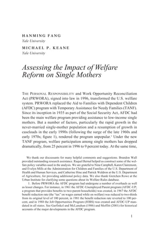
mothers. But a number of factors, particularly the rapid growth in the
never-married single-mother population and a resumption of growth in
caseloads in the early 1990s (following the surge of the late 1960s and
early 1970s; figure 1), rendered the program unpopular.1 Under the new
TANF program, welfare participation among single mothers has dropped
dramatically, from 25 percent in 1996 to 9 percent today. At the same time,

We thank our discussants for many helpful comments and suggestions. Brandon Wall
provided outstanding research assistance. Raquel Bernal helped us construct some of the wel-
fare policy variables used in the analysis. We are grateful to Nina Campbell, Karen Clairemont,
and Evelyn Mills at the Administration for Children and Families of the U.S. Department of
Health and Human Services, and Catherine Hine and Patrick Waldron at the U.S. Department
of Agriculture, for providing additional policy data. We also thank Gretchen Rowe at the
Urban Institute for clarifying some questions about its Welfare Rules database.
1. Before PRWORA the AFDC program had undergone a number of overhauls as well
as lesser changes. For instance, in 1961 the AFDC-Unemployed Parent program (AFDC-UP;
a program that provides benefits to two-parent households) was created, in 1967 the AFDC
benefit reduction rate (the “tax” on wages earned while on welfare) was reduced to two-thirds
from its original level of 100 percent, in 1981 the benefit reduction rate reverted to 100 per-
cent, and in 1988 the Job Opportunities Program (JOBS) was created and AFDC-UP man-
dated in all states. See Garfinkel and McLanahan (1986) and Moffitt (2001) for historical
accounts of the major developments in the AFDC program.

1

2 Brookings Papers on Economic Activity, 1:2004

Figure 1. Welfare Caseloads, 1936–2002a

Millions

14

12 Total recipients

10

8

6

Families
4

2

1945 1955 1965 1975 1985 1995

Source: Administration for Children and Families, Department of Health and Human Services.
a. Annual averages of monthly data on recipients of AFDC (before 1996) or TANF.

the fraction of single mothers who work has increased from 74 percent
in 1996 to 79 percent today. The goal of this paper is to ascertain what fea-
tures of welfare reform, if any, have been most responsible for this decline
in welfare participation and increase in work among single mothers.
Two factors complicate our task. First, a key feature of PRWORA was
that it reduced federal authority over welfare policy, giving the states much
greater leeway in the design of their own individual TANF programs. A
great deal of program heterogeneity has emerged across states, making it
difﬁcult to develop a set of variables that comprehensively characterize the
different state TANF programs. Second, a number of other recent develop-
ments may also have contributed to the changes in welfare and work par-
ticipation since 1996. These factors, such as the strong U.S. economy of
1996 –2000 and the signiﬁcant expansion of the earned income tax credit
(EITC) after 1993, must be controlled for in order to isolate the impact of
particular elements of state TANF policies.

Fang and Keane 3

One important fact lends credence to the idea that factors other than
PRWORA may account for the lion’s share of recent caseload declines: the
dramatic drop in welfare participation (and the dramatic increase in work)
among single mothers actually began in 1993–94, before PRWORA’s
enactment (figure 2). From 1993 to 1996 AFDC participation fell from
32 percent to 25 percent. On the other hand, beginning around 1993, many
states began to obtain federal waivers allowing them to adopt TANF-like
reforms of their AFDC programs. Such reforms included work requirements,
time limits on beneﬁts, sanctions for failure to meet work requirements, and
family caps. These changes may have contributed substantially to caseload
declines even before PRWORA.
At the same time that PRWORA delegated greater control of welfare
policy to the states, it also mandated nationwide many of the popular fea-
tures introduced under state waivers, such as time limits and work require-
ments. To understand the sense in which the federal law “mandates”
certain features of state TANF programs, one must understand how federal

Figure 2. Unemployment and Welfare Participation among Single Mothers, 1980–2002

Percent

Welfare participation
30

25

20

15

10
Unemployment
5

1985 1990 1995 2000
Source: Bureau of Labor Statistics and authors’ calculations based on CPS data.


TANF funds are distributed to the states. Under AFDC, states received
federal matching funds based on their AFDC expenditures. PRWORA
converted these matching funds to block grants. The block grant for a state
was fixed at a level related to federal funding of AFDC benefits and other
related programs in the year when that funding had been highest in that
state. States were given substantial leeway in how the block grant funds
could be used: for example, they may use it to support child care (an impor-
tant postreform development to which we will return). However, to avoid
fiscal penalties on the federal block grant, states must adhere to a “main-
tenance of effort” (MOE) rule: states must maintain their spending on
assistance for needy families at no less than 75 to 80 percent of their pre-
1996 level.2
PRWORA requires that state TANF programs set a five-year lifetime
limit for any individual receiving federally funded aid, although states
may exempt up to 20 percent of their caseload from the limit. States may
elect to set shorter time limits, and many have. However, any assistance
provided to recipients beyond the five-year limit must be financed solely
out of state funds. Three states (Michigan, New York, and Vermont) have
effectively decided not to enforce the five-year limit. And many states
(such as California) do not terminate but only reduce benefits when the
time limit is reached. PRWORA also requires that a specific and rising
percentage of states’ TANF recipients either work or engage in work-
related activities (such as job search or training), and that states impose a
work requirement on any recipient who receives TANF for more than two
years. Again, states may set a shorter work requirement time limit, and
many have done so. States also vary greatly in the sorts of exemptions
from work requirements that they allow and in the penalties they impose
if work requirements are not satisfied.
Roughly contemporaneously with the changes implemented by
PRWORA, the U.S. economy experienced one of its longest postwar expan-
sions. The national unemployment rate remained below 5 percent from
1997 to 2001 and dropped as low as 4 percent in 2000 (figure 2). At
about the same time, the EITC was dramatically expanded in terms of both
the number of recipients and the generosity of the credit. Figure 3 shows

2. Moreover, states may carry TANF funds over from fiscal year to fiscal year without
limit. Although the use of carried-over funds is, in principle, more limited than same-year
funds, in practice, the restrictions do not matter.

Fang and Keane 5

Figure 3. Families Receiving EITC and Aggregate Credits Received, 1975–2002a

Millions Billions of dollars

35
20
30

25
15

20

10
15
Families (left scale)
10
5
5
Credits (right scale)

1980 1985 1990 1995 2000

Source: Internal Revenue Service data and U.S. House of Representatives (2000).
a. Data for 2002 are projections.

that the number of federal EITC recipients increased from about 7 million
in 1980 to 19.6 million in 2001. The federal EITC phase-in rate for a sin-
gle mother with one child increased from 10 percent in 1980 to 34 percent
in 2002.3 Moreover, many states have enacted additional EITC programs
of their own (for more details of the EITC expansion, see the discussion
of the EITC under “Data” below). Other contemporaneous policy changes
include the expansion of Medicaid under the Omnibus Budget Reconcili-
ation Act of 1989 (OBRA 1989), which dramatically expanded health
insurance coverage for low-income women and children who had not been
receiving cash welfare benefits. Moreover, expenditure on the Child Care
and Development Fund (CCDF) increased from $1.4 billion in 1992 to
$7.9 billion in 2001 (figure 4). In fact, the value of child care subsidies

3. The EITC increases in proportion to earned income at the phase-in rate until the credit
reaches the (fixed) maximum amount. The credit starts to decrease at the phase-out rate when
earned income exceeds another fixed threshold.

Figure 4. Expenditure of Child Care and Development Fund and Child Support
Enforcement, 1978–2002

Billions of dollars

8
CCDF
7

6

5

4

3

2
Child Support Enforcement
1

1982 1986 1990 1994 1998

Source: Department of Health and Human Services.

and other noncash benefits now exceeds cash assistance in total federal and
state spending under TANF programs. The federal and state governments
have also substantially increased expenditure for child support enforce-
ment (figure 4). Naturally, all of these changes in the economic and policy
environment could affect the incentives of single mothers to participate in
welfare or work.
The changes in average yearly AFDC/ TANF caseloads over the past
several decades, depicted in figure 1, can be summarized as follows:
— A steep increase in AFDC caseloads occurred in the late 1960s and
early 1970s, which were a time of enormous expansion in government
public assistance programs, including the establishment of the food stamp
and Medicaid programs. Moreover, between 1968 and 1971 the Supreme
Court abolished the absent father rule, the residency requirement, and reg-
ulations that denied aid to families with “employable mothers.” These
rulings increased the welfare take-up rate substantially.

Fang and Keane 7

— AFDC caseloads were almost flat from the early 1970s until 1990,
with a mild increase in the early 1980s due to the back-to-back recessions
of 1980 and 1981–82. The increase in the benefit reduction rate (the “tax”
on wages earned while on welfare) from two-thirds to 100 percent during
President Ronald Reagan’s first term quickly stopped that uptick.
— A dramatic increase in the caseload occurred from 1990 to 1994.
This increase is puzzling because the 1990 –91 recession was quite mild,
and the 1988 Family Support Act had recently mandated that “work eligi-
ble” AFDC recipients participate in welfare-to-work programs. Nor did
the welfare participation rate of single mothers exhibit a steep increase
(figure 2). We discuss various explanations for this phenomenon in our
review of the literature below.
— Welfare caseloads dropped spectacularly after the peak in 1994.
The total caseload fell more than 60 percent from the peak of 1994 to 2002,
a period roughly contemporaneous with the sustained economic expansion
of 1992–2000. The recession that began in March 2001 did increase wel-
fare caseloads in some states, but only slightly, and the national caseload
showed a further slight decrease.

How did the different components of welfare reform and other contem-
poraneous economic and policy changes contribute to the spectacular
drops, both in the welfare participation rate of single mothers and in wel-
fare caseloads, that have occurred since 1993? What were the relative
contributions of time limits, work requirements, the EITC, child care sub-
sidies, and the strong macroeconomy? These are questions of immense
importance for both policymakers and researchers. The answers matter
for the design of improved welfare policies and for understanding how
welfare policies should respond to macroeconomic conditions.
Much research has already been devoted to these questions, and we
review some of the key contributions to this literature in the next section.
All of these have focused on only one or a few of the policy and economic
variables of interest. Thus they are unable to measure the separate contri-
butions of each of the elements mentioned above. Furthermore, we would
argue, studies that focus on only a few policy variables may yield biased
estimates of the effects of the policies in question, because they exclude
other important policy and environmental factors.
One of the main contributions of this paper is the construction of a detailed
data set that includes measures of all the key economic and policy elements


described above, on a state-by-state and year-by-year basis, for the entire
1980 –2002 period. One concern in incorporating so many features in one
grand analysis was the possible collinearity among the policies,4 many of
which were implemented roughly contemporaneously. We deal with this
problem by exploiting both cross-state variation in the timing and form of
particular policies as well as cross-sectional variation in how individuals
with different characteristics are affected differently by seemingly collinear
policies. We discuss in detail the sources of variation that we use to iden-
tity the effects of each variable of interest.
The individual-level data that we use, in conjunction with the economic
and policy variables we compiled ourselves, are those in the Annual Demo-
graphics Supplement to the March Current Population Survey of the U.S.
Bureau of the Census (March CPS).5 From the 1981–2003 supplements
(which cover the period 1980 –2002), we extracted data on all single
mothers with dependent children, or, more specifically, women who were
not living with a spouse at the time of the interview and who had at least
one dependent child age 17 or younger. These women may be divorced,
widowed, separated, or never married, and the children may be their bio-
logical, step-, or adopted children as long as the mother could claim them
as her dependents. Single-mother families are not necessarily single-adult
families, since single mothers may be living with other adults, including,
for example, their parents or their unmarried partners or other related or
unrelated individuals.6
We achieve two main goals in this paper. First, we show that, with a
comprehensive list of control variables that include demographic, eco-
nomic, and policy variables and a rich set of interaction terms, we are able
to develop a model that rather successfully explains both the levels of and
changes in welfare and work participation rates among single mothers
across states, time, and various demographic groups for the whole 1980 –
2002 period. Second, using simulations of the model, we estimate the

4. For instance, Grogger (2003, p. 398) states, “Characterizing each reform is a diffi-
cult enterprise, however, which in conjunction with significant collinearity issues leads me
to take a somewhat less ambitious approach here.”
5. In 2003 the Census Bureau renamed the March CPS the Annual Social and Eco-
nomic Study.
6. Single women with dependent children have been the main recipients of benefits
under both AFDC and TANF. Although single-parent families maintained by fathers, child-
only families, and two-parent families where the primary earner is unemployed may also be
eligible for benefits, single mothers account for a large majority of the caseload.

Fang and Keane 9

contributions of the various components of welfare reform and other
contemporaneous economic and policy changes to welfare and work par-
ticipation rates. Of course, our confidence in our counterfactual decompo-
sition relies, to a large degree, on the success of our empirical model in
fitting the historical data on work and welfare participation rates.
Our main findings can be summarized as follows:
— The key economic and policy variables that contribute to the over-
all 23-percentage-point decrease in the welfare participation rate among
single mothers from 1993 to 2002 are, in order of relative importance,
work requirements (accounting for 57 percent of the decrease), the EITC
(26 percent), time limits (11 percent), and changes in the macroeconomy
(7 percent). This ranking holds for all years since 1997, although the con-
tributions of the different factors differ by demographic group.
— The key economic and policy variables that contribute to the overall
11.3-percentage-point increase in the work participation rate among sin-
gle mothers from 1993 to 2002 are, in order of relative importance, the
EITC (33 percent), macroeconomic changes (25 percent), work require-
ments (17 percent), and time limits (10 percent). However, we find inter-
esting differences in the relative importance of these variables across
demographic subgroups and by time period.
These findings have important policy implications. It seems that although
work requirements are highly effective at getting single mothers off wel-
fare, they are not as effective at getting them to work. Indeed, whether
single mothers work or not after leaving welfare depends crucially on condi-
tions in the macroeconomy. One big success in public policy has been the
expansion of the EITC, which contributes significantly to both getting
single mothers off welfare and getting them to work. Our research high-
lights the crucial difference between “leaving welfare” and “working.”
Indeed, we document the somewhat troubling development that nearly
one-quarter of welfare leavers actually did not start work.
The paper is organized as follows. We begin with a selective critical
review of some influential earlier studies. We then describe both the
individual-level data from the March CPS and the economic and policy
variables that we use in our empirical analysis. Next we give some
descriptive statistics that emphasize the rich interactions between the eco-
nomic and policy variables and the demographic characteristics of single
mothers, and we use these to motivate our empirical model. Following a


description of our empirical specification, we present and interpret our
empirical estimates, discuss the fit of our empirical model, and use the
model to decompose the contributions of different economic and policy
variables to changes in welfare and work participation rates. Finally, we
draw conclusions and suggest directions for future research.

A Selective Review of the Welfare Reform Literature

In this section we discuss critically some of the key papers in the relevant
literature and highlight the differences between their approaches and ours.7

Studies on the Effects of Time Limits
The aspect of the 1996 welfare reform that has received the greatest
attention is the elimination of the entitlement status of welfare, and in par-
ticular the imposition of time limits on welfare receipt. PRWORA created
a five-year lifetime limit on TANF receipt, in the sense that, except in lim-
ited special circumstances, states may not use federal funds to pay TANF
benefits to any adult for more than a total of sixty months during that per-
son’s lifetime. But time limits did not originate with PRWORA. Many
states had already instituted time limits on welfare receipt under federal
waivers. Given the perceived centrality of time limits to the reform strat-
egy, many studies have attempted to estimate the effects of time limits on
welfare participation and other aspects of behavior.
Notable studies of time limits include those of Jeffrey Grogger and
Charles Michalopoulos.8 These papers exploit the fact that, under both
AFDC and TANF rules, only families with children under 18 are eligible
for benefits. Thus time limits should have no (direct) impact on the behav-
ior of single mothers whose children would reach the age of 18 before the
limit could come into play.9 Therefore, in a before-and-after design, any

7. Many interesting and important papers are not discussed in this review. Grogger,
Karolyn, and Klerman (2002) and Blank (2002) provide extensive literature reviews.
8. Grogger (2000, 2003) and Grogger and Michalopoulos (2003).
9. More generally, the strength of the incentive to conserve, or “bank,” eligibility
depends on the age of a woman’s youngest child. If her youngest child is over 13, a newly
imposed five-year time limit does not change her choice set at all. However, if her youngest
child is under 13, then, the younger that child, the greater the option value of preserving wel-
fare eligibility. Thus, ceteris paribus, time limits should enhance work incentives more for

Fang and Keane 11
Table 1. Welfare Participation Rates of Single Mothers, by Age of Youngest Child
Change
Age of Before time After time
youngest child limitsa limits Percentage
(years) (percent) (percent) points Percent
0–6 41.3 23.8 −17.5 − 42
7–12 23.1 13.3 −9.8 − 42
13–17 16.0 11.0 −5.0 −31
All 32.0 18.8 −13.2 − 41
Source: Reproduced from Grogger (2000, table 2). Data are from the March CPS from 1979 to 1999.
a. The year when time limits were introduced varies from state to state.

change in welfare participation among mothers with older children should
be due solely to other time-varying factors besides the imposition of time
limits (such as changes in general economic conditions or in other com-
ponents of welfare reform). The change in participation rates for mothers
with older children thus provides a baseline estimate of the impact of all
these other factors. These mothers can therefore serve as a “control group”
in estimating the effect of time limits. Under the assumption that all other
time-varying factors affect the behavior of mothers with older and younger
children in the same way, any incremental participation rate change among
mothers with younger children isolates the effect of time limits.
Table 1, which is adapted from one of Grogger’s tables, illustrates this
idea.10 A five-year time limit should not have affected the behavior of sin-
gle mothers whose youngest child was between 13 and 17 years old. Thus
the drop in their participation rate from 16 percent to 11 percent should be
attributable entirely to other time-varying factors, such as work require-
ments or macroeconomic conditions. Next consider single mothers whose
youngest child is 6 years old or less. These women are potentially affected
by time limits, since they could use up the maximum five years of benefits
long before their youngest child reaches age 18. Welfare participation
dropped a much larger 17.5 percentage points among this group. Using

single mothers with younger children than for those with older children. Of course, time lim-
its may also have indirect impacts. For instance, if time limits reduce welfare participation
among other groups in society (such as mothers with younger children), this may increase
the stigma of welfare participation, which would indirectly impact participation rates among
mothers with older children.
10. Grogger (2000).


these ﬁgures, we can estimate the impact of time limits using a difference-
in-differences (DD) approach. Of the 17.5-percentage-point drop in par-
ticipation for single mothers with young children, we attribute 5 percentage
points to the other factors besides time limits, since that is the change we
observe for the control group. This leaves 12.5 percentage points as the drop
in welfare participation attributable to time limits. This is a very substan-
tial effect. It implies that 71 percent of the drop in welfare participation
among mothers with young children was due to time limits.
As Grogger hastens to point out, however, this estimate relies on a
number of strong assumptions.11 Most critically, it supposes that all fac-
tors other than time limits have the same impact on single mothers
whether their children are older or younger. This is a very strong assump-
tion, since mothers with younger children differ from mothers with older
children in important ways. To see this, note that table 1 also shows that,
both before and after time limits were imposed, welfare participation rates
were much higher among single mothers with younger children (41 per-
cent before time limits) than among those with older children (16 per-
cent). This alone illustrates the dramatic difference between the two
groups and calls into serious question the assumption that they would be
affected in the same way by other aspects of welfare reform or by the
business cycle.
The fact that the baseline participation rates differ so greatly between
the two groups creates another serious problem for the simple DD approach.
Even if unmeasured time-varying factors did have a common impact
across groups, to use a DD approach we need to know whether the “com-
mon impact” applies when we measure impacts in levels or in percentages.
This point is also illustrated in table 1. The last column shows the per-
centage change in participation rates for each group following the imposi-
tion of time limits. The single mothers with older children had a 31 percent
decline in welfare participation, whereas those with younger children had
a 42 percent decline. So, if one assumes that the unmeasured factors have
a common percentage-change effect across groups, the DD estimate of the
effect of time limits on mothers with younger children is 11 percentage
points. This implies that only 26 percent of the drop in welfare participa-
tion among this group of mothers was due to time limits. Thus time limits

11. Grogger (2000).

Fang and Keane 13

seem much less important when impacts are measured in percentages
rather than levels.12
We contend that there is only one way around this problem, and that is
to do the hard work of trying to measure and control for a rich set of time-
varying factors that may have affected people with different characteris-
tics differently, and to allow for interactions between these factors and
personal characteristics in constructing our model. The DD approach is
not a panacea for dealing with unmeasured time-varying factors when the
treatment and control groups are different, especially when they have dif-
ferent baseline participation rates.13
Recognizing this, Grogger extends the simple DD analysis described
above to control for four specific time-varying factors that he believed
might have different effects on women with younger children than on those
with older children. Those time-varying factors are the unemployment
rate, the minimum wage, the real level of welfare benefits (all measured
at the state level), and a dummy variable for “any statewide welfare
reform.”14 When these factors are controlled for, and state dummy vari-
ables and state-specific quadratic time trends are included, the estimated
impact of time limits on welfare participation for single mothers with
children age 6 and under drops to 8.6 percentage points.15 This is still
49 percent of the overall 17.5-percentage-point drop in participation for
this group.
Thus Grogger’s results imply that time limits were a major factor
driving down caseloads. His estimates of state unemployment rate effects

12. To dramatize the possibility of this bias, consider the following thought experiment.
Suppose that time limits had no effect on welfare participation, but that other, omitted fac-
tors (such as work requirements and work incentives) caused all single mothers to leave wel-
fare. This would lead to a change of 41 percentage points for mothers with children 6 and
under, and 16 percentage points for mothers with children ages 13 to 17. This would yield an
estimate for the effect of time limits of 25 percentage points, when in reality the effect is
zero. If instead it were known that the omitted factors operated on percentage changes rather
than levels, we would get changes of −100 percent for both the first group and the second,
for a (correct) difference of zero. But of course we have no way to know in advance which
specification—levels or percentage changes—is the right one.
13. This criticism actually applies to many recent applications of the DD methodology,
which have often involved situations where the “treatment” and “control” groups are rather
different at baseline.
14. Grogger (2000).
15. We refer to the results in column 1 of table 5 in Grogger (2000), which we take to be
his main results.


are all insignificant, implying that the strong economy over the period did
not play a significant role. His estimates do imply that falling real AFDC/
TANF benefits had a significant impact on mothers with younger chil-
dren. Interestingly, neither the time limit dummy nor the general reform
dummy nor the unemployment rate nor any of his other controls are sig-
nificant for the single mothers with older children. Thus Grogger’s results
apparently attribute the 31 percent drop in welfare participation for this
group to the state-specific time trends. These may be picking up the effect
of the EITC expansion, a general change in “culture,” or some other fac-
tor not controlled for in the model. Indeed, in a later paper that controlled
for EITC expansion, Grogger found an even smaller effect of time limits
on welfare participation: they now accounted for only about one-eighth of
the decline in welfare use and about 7 percent of the rise in the employ-
ment rate since 1993.16 This is rather close to our own estimates, pre-
sented below, of 11 percent and 10 percent for the contributions of time
limits to changes in welfare and work participation.
An important limitation of Grogger’s approach is that all other aspects
of welfare reform are summarized in his “any statewide welfare reform”
dummy variable. This precludes him from estimating the effects of other
specific policy changes. Furthermore, it will not adequately control for omit-
ted factors if other reforms affect different demographic groups differently.
As an example, one specific feature of welfare reform that Grogger omits,
and which could lead to upward bias in his estimates of time limit effects, is
the massive expansion of subsidized day care for low-income families
that occurred largely as a result of PRWORA (figure 4). Under CCDF
rules, funds may not be used to subsidize day care for children over 12 except
in very rare instances (for example, for children with special needs). Hence
the day care expansion should not have affected single mothers whose
youngest child is 13 to 17 years old. And, obviously, subsidized day care
could have a bigger effect on mothers with pre-school-aged children. That
is, the effects of other contemporaneous reforms omitted from the analy-
sis could indeed be age dependent. We note, somewhat facetiously, that if
we chose to ignore time limits rather than day care, we could use table 1
to obtain a DD estimate of the effect of expanded day care spending.17

16. Grogger (2003).
17. Using a structural model of welfare participation and labor supply estimated on data
from the 1980s, Keane (1995) predicted that a policy of subsidizing single mothers’ fixed

Fang and Keane 15

The later analysis of Grogger and Michalopoulos is less subject to
these sorts of criticisms.18 They estimate the effect of time limits using
data from a randomized experiment, the Florida Family Transition Pro-
gram. This was a fairly small experiment in which welfare recipients in
Escambia County, Florida, were randomly assigned to either a treatment
group that was subject to a two- or three-year time limit or a control group
that was not.19 They estimate that the two-year time limit reduced welfare
participation rates among single mothers with youngest children ages 3 to
5 by 7.4 percentage points (from a base rate of 40.3 percent) during the
first two years after the time limit was imposed. This estimate implies sig-
nificant effects of time limits, but it is difficult to translate it into a predic-
tion for the aggregate welfare caseload, for two reasons: first, the estimate
is based on a two-year limit, whereas most states have longer limits, and
second, it conditions on a sample of women who had applied for welfare
in the first place. Thus it tells us nothing about how time limits would
affect entry into welfare.
Furthermore, we do not think it is possible to generalize the significant
effects of time limits in the Florida context to the broader national context.
Dan Bloom, Mary Farrell, Barbara Fink, and Diana Adams-Ciardullo
(BFFA) provide an excellent discussion of how time limits have been
implemented in practice in many states. They state that “as a relatively
small pilot program . . . [the Florida program] was generously funded and
heavily staffed,” and thus, “With small caseloads, workers were able to
have frequent contact with participants.”20 They go on to point out that
“Recipients who came within six months of reaching their time limit and
who were not employed were referred to specialized staff known as ‘tran-
sitional job developers,’ who worked intensively to help these individuals
find jobs. The transitional job developers sometimes met with recipients

costs of working (primarily day care and transport costs) would reduce their AFDC partici-
pation rate from 25 percent to 20.8 percent (a 17 percent decline) and increase their employ-
ment rate by 7 percentage points from a base rate of 60 percent. Thus our prior is that large
effects of day care subsidies are plausible.
18. Grogger and Michalopoulos (2003).
19. A confounding feature of this experiment was that a child care subsidy was also pro-
vided to both groups. Thus the experiment does not estimate the effect of time limits alone.
However, assuming no interaction between child care subsidies and time limits, the differ-
ences between the treatment and the control groups should net out the effects of child care.
20. Bloom and others (2002, p. 140).


several times a week, and they offered employers generous subsidies to
hire their clients.” Finally, BFFA note that “. . . nearly all of those who
reached the time limit had their benefits fully cancelled. Very few exten-
sions were granted; only a handful of cases retained the child’s portion of
the grant; and no one was given a post-time limit subsidized job.”21
This combination of intensive case management and strict enforce-
ment of the time limit is wildly at variance with the norms under TANF.
In fact, BFFA describe a system where, in practice, time limits are only
sporadically enforced because extensions and exemptions are so com-
mon. They note that roughly 44 percent of the caseload reside in states
such as Michigan, New York, and Vermont, which do not have time lim-
its, or California, Maryland, and Washington, which only reduce (rather
than terminate) benefits when the time limit is reached. Furthermore, sev-
eral states, such as Oregon, stop the welfare time clock if a recipient is
participating in required work or work-related activities, and many states,
such as Connecticut, provide liberal extensions of the time limit if recipi-
ents have made a “good faith effort,” which basically means meeting the
requirements of the state TANF plan with respect to work, job search, and
training and avoiding sanctions.
Thus, in many states, time limits are practically irrelevant. A typical
comment is that of the U.S. General Accounting Office: “In Oregon, months
count toward the time limit only if the family fails to cooperate, and the
State has graduated sanctions resulting in a full family sanction for failure
to participate [in required work activities]. Officials told us they do not
expect any families to ever reach the State time limits in Oregon because,
if families are cooperating, they can expect to receive cash assistance
indefinitely (funded by the State after the waiver expires in the year 2002);
if families are not cooperating, their grants will be terminated long before
the time limit is reached.”22 BFFA describe data on 54,148 TANF recip-
ients who had reached the federal five-year time limit by December 2001.
The bulk of these were in Michigan and New York, since these states
implemented TANF relatively early on. But these states do not impose the
federal limit. Of 5,143 recipients in the other states that did nominally
impose time limits, BFFA report that 51 percent continued to receive
TANF benefits under some sort of extension. The most common exten-

21. Bloom and others (2002, p. 142).
22. U.S. General Accounting Office (1998a, p. 55).

Fang and Keane 17

sion criteria were “good faith effort” (in Connecticut, South Carolina, and
Tennessee), “disabled or caring for disabled family member” (in Georgia,
Louisiana, and Utah), “to complete education or training” (in Georgia),
“high unemployment” (in Texas), and “other” (in Ohio).

Studies of Other TANF and TANF-Like Reforms
A number of previous studies have attempted to look more broadly at
the whole range of factors that might drive caseloads. A paper by Rebecca
Blank was a pioneering effort in this direction.23 She examined the evolu-
tion of welfare caseloads by state and by year over the period 1977–95.
Although her data were entirely from the pre-TANF period, a number of
states had already instituted waivers in the early 1990s, making it possible
to examine the impact of a number of TANF-like reforms.
The details of Blank’s speciﬁcation are worth describing, because they
guide much of the subsequent work in this area. Her dependent variable is
the log ratio of a state’s AFDC caseload to the female population age 15
to 44. Given that most AFDC recipients are in this age range, the depen-
dent variable can be taken to approximate the percentage of women in
this age group who participate in AFDC. This variable ranged from 6 to
8 percent over the sample period and was 7.4 percent in 1994. The policy
variables include the state-specific AFDC “grant” for a family of three
(that is, the benefit for a family with no earnings or outside income) and
dummy variables for whether the state had been granted a waiver and, if
so, whether the policies adopted under the waiver included time limits,
enhanced work requirements, fewer exemptions from (or more severe
sanctions for) failure to meet work requirements, or family caps. (A fam-
ily cap is a policy whereby AFDC beneﬁts are not increased by the usual
per-child increment if a woman has an additional child while already on
AFDC). Controls for aggregate economic conditions were the state un-
employment rate (and two lags of this variable), the median wage, and the
20th percentile wage. Blank also controlled for state demographics such
as average educational attainment, the share of the population that were
black, the share that were elderly, the share that were recent immigrants,
and the share of households headed by single females.
Blank’s results imply that caseloads are mildly sensitive to the un-
employment rate: the estimated elasticity of the welfare participation rate
23. Blank (1997).


with respect to a sustained increase in the unemployment rate is roughly
0.25.24 This means that a 3-percentage-point increase in the unemploy-
ment rate would raise the participation rate by about 11 percent after three
years. Her results also imply that participation is quite sensitive to benefit
levels: the estimated elasticity of the participation rate with respect to the
benefit level is 0.56.
Blank’s study has a few notable shortcomings. First, a salient feature
of the data (figure 1) is that the AFDC caseload was quite flat from 1977
through 1989 (in the range of 3.5 million to 3.9 million families). But it
rose sharply in the 1990–93 period (from 3.8 million in 1989 to 5.0 mil-
lion in 1993), peaked in March 1994 at 5.1 million families, and then
began to drop sharply in mid-1994. One might suspect that the bulge was
due to the mild recession of the early 1990s. Before 1990, however, AFDC
caseloads had never exhibited much cyclical sensitivity. In fact, Blank
shows that half of the caseload increase in 1990–94 was due to increases
in child-only and AFDC-UP cases.25 Thus her dependent variable exag-
gerates the increase in the AFDC participation rate among single females
age 15 to 44 during that period. Presumably, an ordinary least squares
(OLS) estimate would attribute this exaggerated increase to the recession,
leading to an overestimate of the effect of unemployment. Despite this,
Blank notes that her model still does not succeed in explaining the increase
in caseloads in 1990–94.
Second, Blank obtains very puzzling results for the effects of specific
reform features. The coefficient on the “any major state welfare waiver”
dummy implies that a waiver reduces the participation rate by roughly

24. The sum of the coefficients on the current and two lags of the unemployment rate is
0.038 (Blank, 1997, table 2). If log(P) = 0.038U, where P is the participation rate and U the
unemployment rate, then the elasticity of P with respect to U is 0.038U. The mean unem-
ployment rate in the data is 6.583 percent, so at this mean the elasticity is 0.25.
25. The increase in AFDC caseloads during 1990–94 may have also been related to the
1986 Immigration Reform and Control Act (IRCA), which legalized 2.7 million undocu-
mented immigrants residing in the United States since 1982, as well as certain seasonal agri-
cultural workers, and made these legalized immigrants eligible for welfare after a five-year
moratorium. Immigrants legalized under IRCA were more likely to be poor than immigrants
who had entered legally, and legalization may have encouraged resident immigrants to apply
for benefits for their children, even if they themselves were barred from aid receipt during
the moratorium. Since most of these immigrants were legalized in 1987 and 1988, the five-
year moratorium on welfare receipt ended by the beginning of 1994 (see MaCurdy, Man-
cuso, and O’Brien-Strain, 2000, 2002).

Fang and Keane 19

11 percent. However, when this is broken down into a set of dummies for
different aspects of waivers, the dummy for whether a state imposed time
limits is insignificant (and has the wrong sign), and work requirements are
insignificant as well. The dummy indicating that a state imposes harsher
sanctions for failure to satisfy work requirements is estimated to have a
significant positive effect on caseloads. The variables estimated to signifi-
cantly reduce caseloads are dummies for reduced JOBS exemptions and
for whether the state imposed a family cap. The latter policy is estimated to
reduce the caseload by roughly 18 percent, which seems highly implausi-
ble. As Blank states, “the impact of family caps on the caseload in the short
run should be minimal. It merely holds benefits constant for women who
are already on the caseload, it does not remove anyone from the rolls.”26
The Council of Economic Advisers (CEA) conducted a similar exer-
cise using state-level data from 1976 to 1996, updated through 1998 in a
second paper.27 These papers use much sparser sets of controls than does
Blank’s 1997 paper. The only nonwelfare factors included in the models
are the current and lagged unemployment rates (along with state and year
dummies). In the 1997 paper, specifications that include only a portman-
teau dummy variable for “any statewide welfare waiver” imply that a
waiver reduces a state’s caseload by roughly 5 percent.28 When dummies
for specific policies are included instead, the estimates are rather impre-
cise. The only clearly significant policy is stricter work requirement sanc-
tions, which are predicted to reduce the caseload by roughly 10 percent.
It should be stressed that a fairly small amount of data underlies these
estimates. For instance, according to Gil Crouse,29 only five states had
implemented benefit time limits by early 1996, with two more doing so in
the second half of 1996. Two states implemented work requirement time
limits in 1994, four more in 1995, and two more in 1996. Stricter work
requirement sanctions were more common. Six states implemented these
before 1995, five more in 1995, and eight more in 1996. Thus it was only
in 1995–96 that a substantial number of states began to implement TANF-
like policies.30

26. Blank (1997, p. 20).
27. CEA (1997, 1999).
28. CEA (1997, table 2, column 3).
29. Crouse (1999).
30. Schoeni and Blank (2000) use CPS data from 1977–99, thus including three years
of post-TANF data. They also disaggregate state-level caseloads by age and educational


The 1997 CEA report notes that a one-year lead of the waiver dummy
is significant. The estimates imply that a waiver reduces the caseload by
roughly 6 percent in the year before it is implemented. The report points
out that this could be an anticipatory effect: the knowledge that welfare
policies will become stricter may deter women from welfare participation
even before the waiver is implemented. But another explanation is based
on policy endogeneity. It is widely accepted that the increase in welfare
caseloads in 1990–93, and the increase in program costs that this induced,
helped create the political momentum that led to implementation of
waivers and ultimately TANF itself.31 However, by the time many states
had implemented waiver policies in 1995–96, and certainly by the time
that most had begun to implement TANF policies in 1997, a rapid decrease
in the caseload had already begun.32 Any misspecified model that fails to
capture the sharp decline in welfare caseloads beginning around 1995—
before the implementation of most TANF-like policies—will tend to attri-
bute these changes to the TANF and waiver dummy variables. The reason
is simply that the model will produce large serially correlated residuals in
the post-1995 period, and any variable that “turns on” in that period will
help absorb those residuals. Thus what the CEA calls a “policy endo-
geneity” problem we prefer to call a misspecification or omitted variables
problem.33 The best way to deal with this problem is to look for additional

attainment. They measure welfare reform using only waiver and TANF dummies, and they
attempt to control for all other factors using a large set of state and time fixed effects (we dis-
cuss their specification further later in the paper). They obtain the puzzling result that TANF
had no significant effect on work participation.
31. For instance, according to the 2000 Green Book (U.S. House of Representatives,
2000, p. 352), “Frustration with the character, size and cost of AFDC rolls contributed to the
decision by Congress to ‘end welfare as we know it’ in 1996. Enrollment had soared to an all
time peak in 1994, covering 5 million families . . . benefit costs peaked in fiscal year 1994 at
$22.8 billion,” and further, “By early 1995, many Governors pressed for a cash welfare
block grant to free them from AFDC rules. The concept of a fixed block grant . . . was
included in reform bills passed by Congress in 1995 and 1996; both were vetoed. But a third
bill that included changes discussed during the 2 years of debate was enacted by Congress in
July 1996 and was signed by President Clinton on August 22, 1996. By the time of TANF’s
passage, AFDC enrollment had decreased to 4.4 million families.”
32. This can be seen quite dramatically in the state-by-state graphs of caseloads over
time presented by Crouse (1999). By our count the graphs provide clear evidence that case-
loads had begun to fall substantially before any implementation of waivers or TANF in at
least thirty-three of the fifty states.
33. Even if policy were endogenous in the sense that increases in AFDC caseloads in
1990–93 induced the implementation of waivers and TANF policies, this would not by itself

Fang and Keane 21

control variables that can successfully explain caseload evolution in the
prereform period. This is the approach we take here.34
It is interesting to note that, in a model with state fixed effects, our ap-
proach would not work. Consistency of OLS requires only that the covari-
ates and the errors be contemporaneously uncorrelated (that is, that the
policy variables be “predetermined”), whereas fixed effects estimators
rely on “strict exogeneity” (that is, a lack of correlation at all leads and
lags). Thus policy endogeneity would lead to inconsistent estimates in fixed
effects models even if the residuals were serially independent. This is a
strong argument for not including state fixed effects if we believe that
policy endogeneity is present.
The CEA models certainly fail to explain both the increase in case-
loads in 1990 –93 and the decline beginning in 1995. Unemployment rate
changes over this period—the only non-welfare-related explanatory fac-
tor in the CEA models—seem inadequate to explain the phenomenon,
given the history of insensitivity of caseloads to unemployment. The 1997
CEA paper notes that “for the 1989–1993 period that saw a tremendous
increase in the rate of welfare receipt . . . changes in unemployment can
only explain about 30 percent of the rise . . . that leaves roughly 70 per-
cent of the rise unexplained by this statistical analysis.”35 Their model
also attributes 34 percent of the decline in caseloads in 1994–96 to “other
unidentified factors.” Thus a key challenge is to develop a model that can
better account for caseload movements over time, particularly the pre-
TANF decline in caseloads beginning in 1995. Unless a model can fit this

bias the estimates of policy effects. Only if the residuals are serially correlated would one get
potential bias in the waiver and TANF coefficients. For instance, suppose that an omitted
variable was driving up caseloads in 1990–93 and then started to drive them down in 1995.
The omission of this variable would generate serially correlated residuals. If one could find
this variable and include it in the model, thus eliminating the serial correlation, the potential
bias would vanish. The fact that the welfare policies were driven by caseload increases in the
early 1990s would be irrelevant.
34. As CEA (1997) notes, another concern is that caseload increases in the early 1990s
varied from state to state. If those states that had the largest caseload increases were most
likely to implement waivers, then the states with the largest residuals in the early 1990s
would be the ones most likely to implement waivers in 1995 and 1996. If the residuals
exhibit persistence, then waivers in 1995–96 would be correlated with the 1995–96 residuals
as well, inducing bias. Again, this can be thought of as a misspecification or omitted vari-
ables bias, since, if one could control for the omitted factor driving caseloads—and inducing
serially correlated residuals–the bias would vanish.
35. CEA (1997, p. 8).


pattern, any effects that it attributes to waiver and TANF policies may be
spurious.
Robert Moffitt argues that the cyclical sensitivity of AFDC caseloads
might have increased over time.36 Thus, unless one takes a stand on the
cyclical sensitivity of the caseload and how it has evolved over time, one
cannot decide how much of the drop in welfare participation after 1994
was due to welfare reform and how much to the strong economy. If only
aggregate data were available, these would leave one with a hopeless
identification problem. However, Moffitt also pointed out that that cross-
state variation in unemployment rates can, in principle, be used to resolve
this problem. One could ask whether caseloads fell more or less in states
where unemployment fell more or less, and one could even identify how
the cyclical sensitivity of caseloads has varied over time, provided one
assumes that it varies in the same way in all states. We today are in a
much stronger position than previous researchers to identify these cyclical
effects, because we can include data from the recession of 2001–02.

Studies of Non-TANF-Related Reform Policies
Other important policy changes that may have influenced the welfare and
work decisions of single mothers in recent years are the expansions of
Medicaid eligibility for low-income families not on AFDC and the expan-
sion of the EITC. As Keane and Moffitt note,37 the fact that single moth-
ers would tend to lose Medicaid eligibility if they left AFDC created an
important work disincentive before 1987. But a series of Medicaid eligi-
bility expansions in 1987–2002 may have reduced this disincentive, by
allowing single mothers with income above the AFDC/ TANF eligibility
threshold to continue to receive Medicaid benefits. Often eligibility for
Medicaid expansions depended on the age of a woman’s children.
Aaron Yelowitz attempted to quantify the effect of Medicaid expan-
sions on work.38 He measured the extent of eligibility expansion by a sin-
gle variable, which he called GAIN%, defined as the difference between
the Medicaid income eligibility threshold under the expansion and the
AFDC income eligibility threshold before the expansion. Identification of
Medicaid expansion effects came from the variation in GAIN% across

36. Moffitt (1999).
37. Keane and Moffitt (1998).
38. Yelowitz (1995).

Fang and Keane 23

states, over time, and across individuals. He used March CPS data from
1989 through 1992 to estimate a probit model for work participation as a
function of GAIN%. To control for other factors that might vary across states
and time, he also included year and state dummies. Yelowitz’s estimates
imply that the Medicaid expansion of 1989–92 led to a 1.2-percentage-
point decrease in welfare participation and a 0.9-percentage-point increase
in labor force participation among single mothers with at least one child
under 15. However, as discussed earlier, for such a strategy to provide a
consistent estimate of the effect of the policy variable in question, one has
to make the strong and likely implausible assumption that all other time-
varying factors, including all omitted policy variables, impact all single
mothers in the same way, regardless of the ages of their children or their
state of residence. Furthermore, we must know a priori whether the omit-
ted time-varying factors affect the work participation of the “control” and
“treatment” groups in terms of levels or percentages. Only then will the
difference-in-differences methodology work.
Bruce Meyer and Dan Rosenbaum have undertaken a more comprehen-
sive study of the effects of a wide range of factors on the work decisions of
single mothers, but their focus is on the EITC.39 They use CPS data for
1984–96 and incorporate changes in the EITC and other tax rates, AFDC
and food stamp benefit levels, welfare time limits (under waivers), Medicaid
expansion, and child care and training expenditures. Meyer and Rosenbaum’s
paper represented a significant advance over previous studies in that it con-
trolled for a wide range of factors. Their empirical specification, however,
did not control for other key TANF-like reforms under waivers, such as
work requirements. Moreover, because their study used data only up to 1996,
they do not address the separate contributions of various components of
the 1996 welfare reform to the subsequent drop in caseloads. Meyer and
Rosenbaum’s estimates imply that changes in the EITC and other tax poli-
cies explain more than 60 percent of the increase in work among single
mothers relative to childless single women in 1984–96. Somewhat unexpect-
edly, their estimates also imply that Medicaid expansions had a nonnegligi-
ble and negative effect on work participation.
We conclude with two general observations about all the studies we
have described. First, they all use only dummy variables (such as whether
or not a state has implemented a time limit) to capture policy effects. This

39. Meyer and Rosenbaum (2001).


is a problem because a time limit or other policy change will most likely
affect rates of entry and exit from welfare, rather than simply inducing an
immediate shift in the level of participation. The effect of such a policy
thus builds gradually over time. In contrast, we explicitly construct mea-
sures of the time elapsed since particular policy changes might have begun
to affect each single mother (based on her state of residence and demo-
graphics), thus allowing policy effects to develop gradually.
Second, all the studies we have described include state dummies to
control for differences in welfare and work participation across states that
the model leaves unexplained. As already mentioned, one reason for not
using state fixed effects is that consistency of the fixed effect estimator
requires the assumption of strict exogeneity, which we believe is invalid
regarding policy changes. Furthermore, Keane and Kenneth Wolpin show
how the use of state fixed effects can lead to seriously biased estimates of
policy effects in a dynamic model.40 For example, in a dynamic frame-
work, a person decides whether to go on welfare or work or invest in human
capital today based not just on benefits today but on expected future ben-
efits as well. Suppose that each state has a typical level of benefit generos-
ity that is persistent over time (for example, that Minnesota always has
higher benefits than Alabama), but that benefits in both states fluctuate from
year to year. These transitory fluctuations in benefits may have little effect
on work and welfare participation decisions, which instead will be primar-
ily driven by the permanent component of benefits. Hence a state fixed
effects estimator may lead one to underestimate the effect of benefit lev-
els. Using simulations of a dynamic model, Keane and Wolpin show that
this problem can be severe.41
For these reasons we choose not to include state fixed effects in our
models. Of course, this may create a problem if our control variables fail
to explain the persistent differences in levels of welfare participation across
states, and instead generate serially correlated residuals by state. If states
with persistently negative residuals for welfare participation tended to
adopt certain policies under TANF, one might falsely infer that these poli-
cies reduced participation. As we show later in the paper, our models do a
reasonably good job of explaining the persistent differences in levels of

40. Keane and Wolpin (2002a, 2002b).
41. Keane and Wolpin (2002a).

Fang and Keane 25

welfare and work participation across states, so that we are not too con-
cerned about this issue.
To summarize, we feel that previous studies of welfare reform suffer
from a number of important limitations. Typically, they examine only a
subset of the many policy and economic environment variables that might
affect welfare and work decisions. They often use state and time dummies
to control for omitted time- and state-varying factors. This procedure is
only valid under the assumption that such omitted factors affect all demo-
graphic groups equivalently and, even if this is true, that the analyst knows
whether the equivalence holds in terms of levels or in terms of percent-
ages. On the other hand, those studies that omit explicit year effects have
not developed models that succeed in explaining the evolution of welfare
participation over time at the national level, let alone broken down by state
and demographic group.

Data

The data set used in this paper combines individual-level data from the
March CPS with data on a rich set of economic and policy variables. In
describing these data, we will also detail the sources of variation that we
exploit to identify the effects of key economic and policy variables.

Individual Data
Our main data source is the series of March supplements to the Current
Population Survey ﬁelded between 1981 and 2003, covering activities in
1980 –2002.42 The CPS is designed to provide a nationally representative
sample by interviewing approximately 60,000 households. The sample
size was increased in 2001 and 2002 to improve estimates of children’s
health insurance coverage by state, for the purpose of allocating federal
funds under the State Children’s Health Insurance Program (SCHIP) estab-
lished in 1997. The CPS asks retrospective questions about demograph-
ics, work activities, and income. Questions about demographic variables,
such as age, refer to the week before the interview; those about income

42. Our CPS sample is extracted using the CPS Utilities produced by Unicon Research
Corporation.


variables with respect to the previous calendar year; and those about work
activity, such as hours worked and major occupation, with respect to both
periods.
Our unit of analysis is families headed by single mothers. Since we
condition on single-motherhood, we take marital status and the presence
of children as exogenous. Of course, changes in welfare rules could affect
marriage and fertility, but existing empirical work suggests that these
effects are small.43
For purposes of constructing a data set on single mothers, it is impor-
tant to note that the CPS is organized around households defined by a
unique address, for example a house or an apartment. A household may
contain more than one family, with the person who rents or owns the
house considered the head of the household. We select female-headed
families or subfamilies as the unit of analysis.44 We then count the number
of dependents in each female-headed family or subfamily. Note that the
dependent children are not necessarily the woman’s biological children.
Stepchildren or adopted children, grandchildren, and other unrelated chil-
dren whom the woman lists as dependents are also counted.
The CPS survey asks the respondent to provide detailed demographic
information (including age, race, education, and marital status) for every
household member. We construct the age composition of the woman’s
children by counting the number of dependent children at each age. This
is an important step because, as we discuss below, whether a woman is
subject to particular welfare rules (such as work requirements) or eligible
for particular benefits (such as child care subsidies) often depends on the
precise ages of her children.
We construct our welfare utilization measures from the family’s reported
sources of income over the previous calendar year, and we analyze work
participation decisions based on the average hours worked in that year.
Specifically, we consider a single woman a welfare recipient if her income

43. See Moffitt (1992).
44. Specifically, a woman selected into our analysis must satisfy two conditions. First,
she must be the head of the primary family or a subfamily, which also means that she must
have dependent children. This is ensured by selecting the Unicon recode variable _hhrel to
equal 1, 3, 5, 8, 10, 13, 15, 18, 20, 23, 26, 30, 32, 35, 38, 41, or 43. Second, her marital sta-
tus, given by the Unicon recode variable _marstat, must be either 3 (separated), 4 (wid-
owed), 5 (divorced), or 6 (never married).

Fang and Keane 27

from public assistance (Unicon recode variable incpa) is positive.45 The
employment variables come directly from the CPS, which includes the
“hours worked per week last year” (hrslyr). We recorded a woman as work-
ing full-time if she works for thirty-two hours or more a week, and part-
time if she works between eight and thirty-two hours a week.

Policy Data
COMPONENTS OF WELFARE REFORM. An important contribution of the
paper is the comprehensive documentation of the many welfare policy
changes that occurred at the state level over the 1980–2002 period. We
collected detailed information about states’ policies from many different
sources.46 The rest of this section describes the different policy compo-
nents in detail.
Time Limits. PRWORA prohibits states from using federal TANF
funds to provide benefits to adults beyond a sixty-month lifetime time
limit (except that 20 percent of a state’s caseload may be exempted).
Many states have opted for shorter time limits, whereas others have opted
to use their own funds to provide benefits beyond the federal limit. Some
states implemented their own time limits under waivers before PRWORA
was enacted.47
To understand the set of variables we use to capture the possible effects
of time limits, it is useful to examine the theory of how time limits can
affect behavior. A key point is that time limits may have both anticipatory

45. The exact wording varies by year, but the essence of the question is, “How much
did . . . receive in public assistance or welfare in the previous year?” and the answer is coded as
incpa. From 1988 on, the survey also asks about the number of months in which public assis-
tance or welfare is received. Note that incpa will capture cash assistance but not in-kind assis-
tance, such as food stamps.
46. Sources include the State Policy Documentation Project, the U.S. General Account-
ing Office (1997, 1998a), Gallagher and others (1998), Johnson, Llobrera, and Zahradnik
(2003), Hotz and Scholz (2002), the U.S. Department of Health and Human Services (includ-
ing its Office of Family Assistance), the U.S. Department of Agriculture, the Center for Law
and Social Policy, the Urban Institute, the Bureau of Labor Statistics, the National Governors’
Association, the Center on Budget and Policy Priorities, various issues of the U.S. House of
Representatives’ Green Book, the Internal Revenue Service, and various state TANF policy
handbooks.
47. A distinction is sometimes made between when a state implemented its TANF plan
and when it began counting months toward time limits. Arkansas, California, Ohio, and Ore-
gon started counting months toward time limits well after their initial TANF implementation
dates. We use the actual counting date as the effective date for time limits in our analysis.


and direct effects. The direct effect arises simply from the fact that a per-
son who reaches the time limit becomes ineligible for further benefits
(assuming the limit is enforced). The anticipatory effect is subtler. The
basic idea is that a forward-looking person faced with time-limited wel-
fare benefits should try to conserve (or “bank”) her months of eligibility
and use them only when truly necessary.
Consider a simple framework where a woman decides each month
whether to receive welfare or go to work. A myopic person who maximizes
current income would choose to participate in welfare so long as it gener-
ated one dollar more in income than she could earn by working (net of the
cost of working). But a forward-looking person would choose welfare over
work only if the gap between benefits and earnings were substantial. Why
use up a month of welfare eligibility just to get a few extra dollars? In
some future month she may confront a situation where only very low pay-
ing jobs are available, so that welfare benefits far exceed her potential
earnings. It is therefore best to conserve her months of welfare eligibility
for such circumstances.
Stated more formally (see appendix A), in a dynamic framework, such a
woman should make welfare participation decisions by comparing the
value of current-period welfare benefits with the value of current-period
potential earnings plus the option value of conserving a month of benefit
eligibility. As Grogger and Michalopoulos point out, this option value is,
ceteris paribus, an increasing function of the time horizon over which ben-
efits may be used (that is, the number of years until the woman’s youngest
child reaches 18).48 It is also, ceteris paribus, a decreasing function of the
stock of remaining months of eligibility (that is, the option value of pre-
serving a month of eligibility is greater when one has only one month left
than when one has sixty).
Our empirical models include several variables designed to capture
both the direct and the anticipatory effects of time limits—both those cre-
ated under TANF and those created earlier under AFDC waivers. These
variables and others used in the study are defined in table C1 in appen-
dix C. Each variable has up to three subscripts: i for individual, s for state,
and t for year. Thus the subscripts enable one to see whether each variable
varies across states, across people, or both.

48. Grogger and Michalopoulos (2003).

Fang and Keane 29

At the most basic level, we include a dummy variable for whether a
state imposed a time limit in a given year (DTLst ), as well as a dummy for
whether the time limit could have been binding for a particular woman
(DTL_HITist ), given the ages of her children. A woman whose oldest
child is x years old cannot have received welfare for more than x years.
The time limit cannot bind for this woman unless x exceeds the limit,
regardless of how many years ago her state implemented time limits. Thus
the year in which time limits may first bind varies across women in the
same state.
Note that DTLst captures an anticipatory effect of time limits, and
DTL_HITist a direct effect. We also include variables that allow the antic-
ipatory and direct effects of time limits on welfare and work decisions to
develop gradually over time. First, we construct a variable called “months
elapsed since the implementation of time limits” (MONTH_SINCE_
TL_STARTst ). Second, we construct for each single mother a variable
called “months elapsed since the time limits could ﬁrst potentially bind”
(MONTH_SINCE_TL_HITist ).
To evaluate the importance of the anticipatory effect of time limits, we
construct two more variables motivated by the theory presented in appen-
dix A. First, the option value of banking welfare eligibility increases with
the time horizon over which a woman will be categorically eligible for
benefits. This is the remaining time until her youngest child will reach
age 18. We call this variable REMAINING_CHILD_ELIGist. Second, the
option value of banking welfare eligibility decreases with the stock of
eligible months that a woman currently possesses. We call this variable
REMAINING_TL_ELIGist. To construct this measure, we first calculate
the maximum number of months that a woman could have received wel-
fare since her state started her “clock.” Subtracting this from the state time
limit tells us the minimum stock of months that the woman possesses.
At this point it is worth commenting on our overall strategy in con-
structing covariates. We assume that a woman’s demographics, the wel-
fare policy rules she faces, and the economic environment in her state are
all exogenous. Thus, to maintain a true reduced-form speciﬁcation, every
covariate we use as a determinant of welfare or work participation should
be a function of these demographic, policy, and economic environment
variables. One can see the effect of this strategy quite clearly by looking
at how we constructed covariates to measure the effects of time limits. For
instance, we do not want to use a woman’s actual welfare participation


history to construct the remaining months on her time limit clock, because
actual participation decisions are endogenous. Similarly, in the construc-
tion of REMAINING_CHILD_ELIGist, we ignore the fact that a woman
can always extend her months of categorical eligibility by having another
child. REMAINING_CHILD_ELIGist is a function only of a woman’s cur-
rent demographics and state policy variables, so it is certainly an exoge-
nous variable driving current decisions.
A key point is that Michigan, New York, and Vermont have chosen to
use state funds to provide benefits to families beyond the sixty-month fed-
eral limit.49 In other words, these states do not have effective time limits.50
This is a key source of variation in the data that helps identify the effect of
time limits on welfare and work participation. To preview our finding that
time limits have had small effects on welfare participation, we note that,
in Michigan, the number of families on welfare dropped by 58 percent
from August 1996 to June 2002, while the number of individual recipients
dropped by 62 percent. Over the same period the number of families on
welfare in New York dropped by 63 percent, while the number of recipi-
ents dropped 68 percent. These declines are close to the national average,
suggesting that time limits are not the main factor underlying the dramatic
drop in welfare participation since 1996.
Another important source of variation across states is the penalty that is
imposed when a time limit is reached. Among states with effective time
limits, six (Arizona, California, Indiana, Maine, Maryland, and Rhode
Island) continue to provide the child portion of benefits to families even
after the time limit is reached. As we discuss in appendix A, this substan-
tially reduces the impact of time limits. Therefore we constructed a measure
for each state of how benefits are reduced when the time limit is reached.

49. A common mistake in the literature, and in some data sources as well, is to assume
that New York has a sixty-month life time limit. According to the New York State Comp-
troller’s Office, after the TANF time limit is reached, the state will provide Safety Net Assis-
tance (SNA) to the family in the same amount as the family’s TANF grant. Twenty percent
of the monthly payment standard is paid in cash for a personal needs allowance, and the rest
is given on a noncash basis. Thus New York does not have a true time limit.
50. As already discussed, Oregon has a formal time limit, but it, too, is irrelevant because
anyone who satisfies the work requirement for a given month does not have that month count
toward the time limit, and anyone who does not satisfy the work requirement has benefits ter-
minated immediately. Very recently, Arizona and Massachusetts have revised their TANF
plans to use state funds to provide benefits to families beyond the sixty-month federal limit.
This change is too recent to be relevant for our empirical work.

Fang and Keane 31

Work Requirements and Exemptions. Under PRWORA, states must
require parents who receive TANF assistance to participate in “work
activities” after a maximum of twenty-four months.51 Many states have
chosen to adopt shorter work requirement time limit clocks. States adopted
their first TANF plans over the period from October 1996 through Janu-
ary 1998 and adopted revised TANF plans roughly two years later. Under
the initial TANF plans, twenty states required benefit recipients to start
participating in work activities immediately. Under the revised TANF
plans, twenty-five states required immediate work participation. Most states
that do not impose an immediate work requirement have adhered to the
twenty-four-month maximum allowed under the federal law. The require-
ment that recipients participate in work activities may increase the disutil-
ity of welfare participation, leading to reductions in welfare caseloads and
increased work among single mothers.
Section 407, paragraph (b)(5), of PRWORA gives states the option to
exempt single parents with a child up to 1 year of age from work require-
ments. However, many states, such as California, have chosen to exempt
only those single mothers with children under 3 or 6 months of age, and a
few have granted longer exemptions. Thus there is considerable variation
in the variable we call “age of child exemption from work requirements”
(CHILD_EXEMPT_AGEst). We use this variable, in conjunction with the
state-specific work requirement time limit and the age of the women’s
youngest child, to construct an indicator for whether a woman could be
subject to a work requirement. We call this variable SWRist.
Thus we have two key sources for the identification of the effects of
work requirement time limits. First, because of the variation in when states
implemented their TANF plans and in the length of their work requirement
time limit clocks, there is substantial variation across states in how early a
single mother could have been subject to binding work requirements. For
instance, under AFDC waivers, work requirements could have come into
force as early as mid-1994 in Iowa, October 1995 in Michigan, and mid-

51. Work activities as defined in PRWORA include “(1) unsubsidized employment;
(2) subsidized private sector employment; (3) subsidized public sector employment; (4) work
experience (including work associated with refurbishing of publicly assisted housing); (5) on-
the-job training; (6) job search and job readiness assistance; (7) community service pro-
grams; (8) vocational educational training; . . . and (12) the provision of child care services
to an individual who is participating in a community service program.”


1996 in Wisconsin. TANF work requirements could have been binding as
early as the fall of 1996 in Alabama, Connecticut, Florida, Indiana, Kansas,
Nebraska, New Hampshire, Oklahoma, Oregon, and Utah. On the other
hand, work requirements were not binding until December 1998 in New
York, January 1999 in Louisiana, February 1999 in New Jersey, March
1999 in Pennsylvania, and July 1999 in Illinois, Minnesota, and Missouri.52
Second, as already noted, we can exploit individual variation based on
children’s ages. For example, assume that two otherwise similar women
living in different states have both been on TANF long enough to have
reached their state’s work requirement time limit. Suppose that each has a
youngest child who is 9 months old. Suppose further that their states have
similar policies, except that one state exempts women with children under
12 months old and the other exempts only women with children under
6 months old. Then only the woman in the ﬁrst state is exempt from the
work requirement, and any difference in welfare participation and work
behavior between these women will provide additional evidence on the
effects of work requirements. Similarly, take two otherwise similar women
living in different states, each of whom has just one child, who is 18 months
old. Suppose their states have similar policies, except that one imposes an
immediate work requirement whereas the other imposes a work require-
ment only after twenty-four months on welfare. The woman in the first
state may be subject to a work requirement, but the woman in the second
cannot be. Since her only child is only 18 months old, she cannot yet have
been on welfare for twenty-four months.53
Besides the exemption based on age of youngest child, many states allow
other exemptions from work requirements under TANF. These include
exemptions for single parents with children under age 6 who are unable to
obtain child care, and for recipients who are disabled or have a disabled

52. We calculate that the fraction of women who were potentially subject to a work
requirement (SWR = 1) was 5 percent in 1995 and then rose to 16 percent in 1996, 46 percent
in 1997, 62 percent in 1998, 85 percent in 1999, and 91 percent in 2000. It then stabilized at
about 91 percent in 2001–02.
53. It is important to understand how the exemption for age of youngest child interacts
with the work requirement time limit clock. Suppose that a state has a twenty-four-month
time limit and that mothers whose youngest child is less than 12 months are exempt. If a
woman is on welfare starting from the time the child is born, then when the child reaches
1 year of age she will have just 1 year left on the clock.

Fang and Keane 33

household member.54 We call the total number of these exemptions
N_WR_EXEMPTIONst. States also differ as to whether they impose a
full or a partial benefit sanction if a recipient does not satisfy the work
requirement. A “partial” sanction generally means that only the adult por-
tion of benefits, and not the children’s portion, is denied. In 1996 nine
states imposed a full sanction. That number increased to twenty-three in
1997 and stayed close to thirty from 1998 onward. We call the dummy
variable indicating imposition of a full sanction DFULLSANCTIONst.55
We view both the sanction variable and the exemption variable as indica-
tors of the strictness with which a state enforces its work requirement time
limit, and we interact the work requirement variables with these measures
of strictness.56
Finally, work requirements can, in theory, have anticipatory effects
just as time limits do. If a state adopts a work requirement with a twenty-
four-month time limit before the requirement is triggered, this creates an
incentive to avoid welfare participation even before the twenty-four
months is used up. One reason is to conserve time on the clock. Another
reason is that, since the time limit reduces expected future welfare partic-
ipation, it increases the value of human capital investment today. Thus we
also include in our models a dummy for whether a state has a time limit in
effect (DWORKREQst).
Benefit Reduction Rates and Earnings Disregards. The AFDC program
always imposed a “tax” on a recipient’s earnings while on welfare, called
the benefit reduction rate (BRR). Allowance was made for deductions for

54. States must maintain certain work participation rates among TANF recipients in
order to avoid penalties to their TANF block grants. Originally, 25 percent of all families
receiving assistance were required to participate in work activities for at least twenty hours a
week. The required rate was gradually raised to 50 percent in 2002, and the hours requirement
was raised to twenty-five hours in 1999 and thirty hours in 2000. However, these require-
ments were relaxed for states that achieved substantial caseload reductions. Because case-
loads fell so dramatically after 1996, states were rarely subject to significant participation rate
requirements.
55. States often have a more lenient sanction policy for first-time violators of work
requirements. Although we have information about these first-time sanction rules, we use only
the “ultimate” sanction rule in our analysis. There is a high correlation between the first-time
and ultimate sanctions.
56. Pavetti and Bloom (2001) classify twenty-five states as “strict” and thirteen as “lenient”
in terms of the benefits denied to families of noncompliant individuals. Their classification is
roughly consistent with our direct classification of states with full versus partial sanctions.


work and child care expenses, and over the history of the AFDC program
the amounts of these work expense deductions were changed several times,
as was the BRR itself. Notably, the BRR was decreased from 100 percent
to 67 percent in 1967, but it was raised back to 100 percent in 1982. Start-
ing that year the work expense deduction was set at $90 a month, and an
additional child care expense deduction was introduced.
In addition, in an effort to encourage work among participants, the
AFDC program at various times in its history included “earnings dis-
regards.” That is, for a specified time after an AFDC recipient started a job,
a part of her earnings (above and beyond the work and child care expense
deductions) would not be subject to the BRR. In general, this earnings
disregard consisted of a fixed component (for example, the first $30 of
monthly earnings) and a variable component (for example, one-third of
earnings beyond the first $30) and applied only during the first several months
of work.57 Starting in late 1992, again in an effort to encourage work, many
states used waivers to enhance their earnings disregards. PRWORA did
not mandate specific disregard policies, and, as a result, substantial hetero-
geneity has emerged in how states set disregards. Many states have ex-
panded disregards and allowed them to apply indefinitely. For instance,
under its TANF plan implemented in January 1998, California set the fixed
portion of the monthly disregard at $225 and the variable portion at 50 per-
cent, with no phase-out over time. Since the variable part of the disregard is
not phased out, it acts just like a BRR of 50 percent, and this is in fact how
we code it. Across states, as of 2002, fixed disregard amounts varied from
zero to $252, and variable disregards ranged from zero to 100 percent.
Obviously, earnings disregards, the BRR, and work expense deduc-
tions directly affect a woman’s incentive to work by altering her effective
after-tax wage rate. A lower effective tax rate makes welfare receipt more
attractive. Furthermore, as we discuss in appendix A, effective tax rates
also affect the incentive to bank months of eligibility when time limits are
present. The higher the effective tax rate, the greater the incentive to forgo
participating in welfare in a month when work can be found.

57. After 1982 the rule was as follows: For each of the first four months of work, the first
$30 of earned income, plus one-third of the remainder, was disregarded when calculating the
monthly benefit. After four months and until one year, only the $30 monthly disregard con-
tinued. After one year there was no earnings disregard. This means that, after one year, a
recipient’s grant amount was reduced by one dollar for every dollar she earned above the
$90 work expense deduction.

Fang and Keane 35

Diversion Programs. Under TANF many States have developed “diver-
sion” programs under which new TANF applicants can receive a few months’
worth of benefits up front if they agree not to participate in TANF for
some stated period of time. A typical program may offer three months of
benefits up front to a person who agrees to stay off “welfare” for three
months. We view this as largely an accounting device to make TANF
caseloads appear smaller, and so we code such diversion payment recip-
ients as welfare recipients. Eight states, however, have introduced what
we regard as genuine diversion programs, whereby TANF applicants
agree to stay off welfare for an extended period in return for short-term
cash payments (or loans) whose value is well below the maximum value
of the forgone benefits.58 In the empirical analysis we simply introduce a
dummy variable to indicate whether the woman lives in a state with a
genuine diversion program.
Child Support Enforcement and Treatment of Child Support Income.
Although nonpayment is widespread, child support is an important source
of income for single women with dependent children (see table 4 below).
Under AFDC, recipients were required to assign child support collections
to the welfare agency. States were then required to pass through the ﬁrst
$50 of monthly child support payments to the family. This pass-through
income was disregarded for purposes of beneﬁt calculation. Between Jan-
uary 1993 and August 1996, states requested and received waivers of a
number of AFDC provisions related to child support enforcement. These
waivers sometimes involved changing the pass-through amount or allow-
ing single mothers to keep child support payments, in which case they
would be subject to certain disregards just like earned income. Under
TANF, all states have discretion to set their own policy in terms of pass-
through or disregard of child support payments.
The Child Support Enforcement and Paternity Establishment (CSE)
program was enacted in 1975 to address the problem of nonpayment of
child support owed by noncustodial parents. CSE has programs to help
locate absent parents and establish paternity. The CSE administrative expen-
diture is an important indication of how likely it is that a single woman will
be able to collect child support. Figure 4 showed the large increase in CSE
expenditure from $2.9 billion in 1996 to $5.1 billion in 2002, a 76 percent

58. These eight states are Arkansas, Florida, Kentucky, Idaho, Montana, Texas, Wash-
ington, and Wisconsin.


jump. To measure state-level CSE activity, we take state-level CSE expen-
diture and divide it by the state population of single mothers (excluding
widows).59 This, combined with variation in CSE spending across states
and over time, provides the three key sources of variation that identify
the effect of child support enforcement expenditure on welfare and work
participation.
In terms of the incentives created, there are important interactions be-
tween CSE expenditure and the pass-through and disregard rules. Since
child support payments are heavily taxed under TANF rules in many
states, enhanced child support collections provide an incentive to avoid
welfare. On the other hand, enhanced pass-throughs or disregards may
reduce this incentive.
Child Care Subsidies and the Child Care and Development Fund. In
the late 1980s several new programs expanded federal support for child
care. The Family Support Act of 1988 created two programs, AFDC
Child Care and Transitional Child Care. AFDC Child Care was designed
as an entitlement for single parents on AFDC who were working or
enrolled in job training or education programs. Transitional Child Care
provided a temporary child care subsidy to single parents with young chil-
dren for twelve months after they left AFDC to start working. Both pro-
grams used AFDC participation as an eligibility criterion. The Omnibus
Budget Reconciliation Act of 1990 (OBRA 1990) created the Child Care
and Development Block Grant and the At-Risk Child Care program.
These programs gave states funds with which to subsidize child care for
low-income working families who were not on AFDC. However, unlike
AFDC Child Care and Transitional Child Care, these beneﬁts were not an
entitlement. PRWORA consolidated these four preexisting programs into
the Child Care and Development Fund. The CCDF provides federal funds
to the states to use in providing child care subsidies to low-income work-
ing families, whether or not these families are current or former TANF
recipients. Under the CCDF a great deal of heterogeneity has emerged in
the design of states’ child care subsidy programs. In particular, many states
ration beneﬁts, and states differ in terms of whether they give priority to
low-income families who are on TANF or just transitioning off TANF.

59. CSE expenditure should not impact the work or welfare decisions of widows, who
do not have ex-husbands from whom to collect alimony or child support.

Fang and Keane 37

We use state CCDF expenditure per single mother as a measure of the
availability and generosity of child care subsidies in a state. A key factor
identifying the effect of these subsidies is that they are essentially irrelevant
for women whose children are older than 12, since they are not eligible for
subsidies except in rare instances (for example, for children with special
needs). Also, the effect of child care subsidies is presumably stronger for
women whose children are not yet of school age.
As we discuss in appendix B, an important aspect of PRWORA is the
maintenance-of-effort requirement, which requires each state to maintain
spending on assistance for needy families at a minimum of 75 percent of
its pre-1996 level in order to receive the full TANF block grant. The MOE
requirement interacts with the CCDF in an important way. The CCDF
funding system is rather complex, consisting of federal funds to which
states are entitled, plus federal matching funds that require state contribu-
tions, plus discretionary state contributions, including a certain level of
funds that states are allowed to transfer out of the TANF block grant. But
the key point is that the state part of CCDF spending counts as MOE
spending. Thus, when welfare caseloads began to drop unexpectedly rapidly
after 1996, causing state spending on TANF cash assistance to drop, the
states shifted substantial resources into the CCDF as one way to achieve
the MOE requirement. This dynamic was partly responsible for the rapid
growth in total expenditure on CCDF from 1996 to 2002 (ﬁgure 4).
An alternative to using CCDF expenditure per single mother as a mea-
sure of the generosity of a state’s child care program would be to use
detailed program parameters, such as the monthly income limit for eligi-
bility and the co-payment rate, which are state-specific and have varied
over time within states. We choose not to use this approach because of the
problems created by rationing. A state with a seemingly generous program
(for example, a high income eligibility threshold and a low co-payment)
will tend to have a longer waiting list. Thus program generosity is more
accurately measured by the state’s actual expenditure per case than by the
income eligibility threshold and co-payment rates.
CONTEMPORANEOUS POLICY CHANGES. Our data set also contains de-
tailed information about state policies other than those directly related to
AFDC and TANF.
Earned Income Tax Credit. The EITC, enacted in 1975, is a refund-
able federal income tax credit that supplements wages for low-income
working families. Major expansions of the EITC occurred in 1986, 1991,

Grants and Outcomes

Recommandé

Recommandé

Contenu connexe

Tendances

Tendances (20)

En vedette

En vedette (8)

Similaire à Grants and Outcomes

Similaire à Grants and Outcomes (20)

Plus de pleasure16

Plus de pleasure16 (20)

Dernier

Dernier (9)

Grants and Outcomes