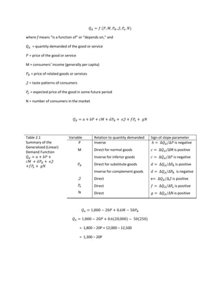
1. where f means “is a function of” or “depends on,” and
= quantity demanded of the good or service
= price of the good or service
M = consumers’ income (generally per capita)
= price of related goods or services
= taste patterns of consumers
= expected price of the good in some future period
N = number of consumers in the market
Table 2.1 Variable Relation to quantity demanded Sign of slope parameter
Summary of the P Inverse is negative
Generalized (Linear)
M Direct for normal goods is positive
Demand Function
Inverse for inferior goods is negative
Direct for substitute goods is positive
Inverse for complement goods is negative
Direct e is positive
Direct is positive
N Direct is positive
= 1,800 – 20P + 12,000 – 12,500
= 1,300 – 20P

2. TABLE 2.2 Price Quantity Demanded
The Demand Schedule for the $65 0
Demand for the Demand
60 100
Function
50 300
40 500
30 700
20 900
10 1,100
TABLE 2.3 (1) (2) (3) (4)
Three Demand
Schedules Quantity demanded Quantity demanded Quantity demanded
Price (M = $20,000) (M = $20,000) (M = $19,500)
$65 0 300 0
60 100 400 0
50 300 600 0
40 500 800 200
30 700 1,000 400
20 900 1,200 600
10 1,100 1,400 800
TABLE 2.4 Determinants of demand Demand Demand Sign of slope
Summary of increasesa decreasesb parameterc
Demand Shifts 1. Income (M)
Normal good M rises M falls c > 0
Inferior good M falls M rises c < 0
2. Price of related good (
Substitute good falls d > 0
Complement good falls rises d < 0
3. Consumer tastes ( ) rises falls e > 0
4. Expected price ( rises falls f > 0
5. Number of consumers (N) N rises N falls g > 0
a
Demand increases when the demand curve shifts rightward.
b
Demand decreases when the demand curve shifts leftward
c
This column gives the sign of the corresponding slope parameter in the generalized demand function.

3. SUPPLY
In general, economists assume that the quantity of a good offered for sale depends on six major
variables”
1. The price of the good itself.
2. The price of the inputs used to produce the good.
3. The prices of goods related in production.
4. The level of available technology.
5. The expectations of the producers concerning the future price of the good.
6. The number of firms or the amount of productive capacity in the industry.
Table 2.5 Variable Relation to quantity supplied Sign of slope parameter
Summary of the P Direct is positive
Generalized (Linear) Inverse l is negative
Supply Function Inverse for substitutes in
production (wheat and corn) is negative
Direct for complements in
production (oil and gas) is positive
Direct is positive
Inverse is negative
F Direct is positive
TABLE 2.6 Price Quantity Demanded
The Supply Scheduled for the $65 750
Supply Function
60 700
50 600
40 500
30 400
20 300
10 200

4. TABLE 2.7 (1) (2) (3) (4)
Three Supply
Schedules Quantity supplied Quantity supplied Quantity supplied
Price ) ) )
$65 750 900 450
60 700 850 400
50 600 750 300
40 500 650 200
30 400 550 100
20 300 450 0
10 200 350 0
TABLE 2.8 Determinants of supply Supply Supply Sign of slope
Summary of increasesa decreasesb parameterc
Supply Shifts 1. Price of inputs ( l < 0
2. Price of goods related in production
(
Substitute good m < 0
Complement good m > 0
3. State of technology (T) T rises T falls n > 0
4. Expected price ( falls r < 0
5. Number of firms or productive
capacity in industry (F) F rises F falls s > 0
a
Supply increases when the supply curve shifts rightward.
b
Supply decreases when the supply curve shifts leftward.
c
This column gives the sign of the corresponding slope parameter in the generalized supply function
TABLE 2.9 (1) (2) (3) (4)
Market Excess supply (+) or
Equilibrium Quantity supplied Quantity demanded excess demand (-)
Price )
$65 750 0 +750
60 700 100 +600
50 600 300 +300
40 500 500 0
30 400 700 -300
20 300 900 -600
10 200 1,100 -900