1. LETTER doi:10.1038/nature10666
Polar methane accumulation and rainstorms on Titan
from simulations of the methane cycle
T. Schneider1, S. D. B. Graves1, E. L. Schaller2 & M. E. Brown1
Titan has a methane cycle akin to Earth’s water cycle. It has lakes in the local rates of precipitation (P) and evaporation (E), with horizontal
polar regions1,2, preferentially in the north3; dry low latitudes with diffusion as a simple representation of slow surface flows from moister
fluvial features4,5 and occasional rainstorms6,7; and tropospheric to drier regions. We show zonal and temporal averages from a simu-
clouds mainly (so far) in southern middle latitudes and polar lation in a statistically steady state, which does not depend on initial
regions8–15. Previous models have explained the low-latitude dry- conditions except for the (conserved) total methane amount present in
ness as a result of atmospheric methane transport into middle and the atmosphere-surface system (here, the equivalent of 12 m liquid
high latitudes16. Hitherto, no model has explained why lakes are methane in the global mean if all methane were condensed at the
found only in polar regions and preferentially in the north; how surface). See Supplementary Information for details.
low-latitude rainstorms arise; or why clouds cluster in southern In the statistically steady state, our model shows an annual- and
middle and high latitudes. Here we report simulations with a three- global-mean methane concentration in the atmosphere corresponding
dimensional atmospheric model coupled to a dynamic surface to 7 m liquid methane—possibly higher than, but broadly consistent
reservoir of methane. We find that methane is cold-trapped and with, observations23,24. The remainder is at the surface. Methane has
accumulates in polar regions, preferentially in the north because accumulated near the poles (Fig. 1a). It is transported there from
the northern summer, at aphelion, is longer and has greater net spring into summer by a global Hadley circulation (Fig. 1b), with
precipitation than the southern summer. The net precipitation in ascent (Fig. 2) and a precipitation maximum (Fig. 1c) over the summer
polar regions is balanced in the annual mean by slow along- pole. Some of the methane accumulating near the summer pole flows
surface methane transport towards mid-latitudes, and subsequent along the surface (on Titan it may also flow beneath the surface2)
evaporation. In low latitudes, rare but intense storms occur around towards mid-latitudes. It evaporates and is transported back towards
the equinoxes, producing enough precipitation to carve surface the opposite pole when the circulation reverses, around equinox. Polar
features. Tropospheric clouds form primarily in middle and high regions lose methane from late summer to winter, with zonal-mean net
latitudes of the summer hemisphere, which until recently has been evaporation rates (E 2 P) reaching around 0.2 m yr21 (1 yr referring to
the southern hemisphere. We predict that in the northern polar 1 Earth year) in the southern summer (Fig. 1b). This is consistent with
region, prominent clouds will form within about two (Earth) years observations: the zonal-mean evaporative loss rate is of similar mag-
and lake levels will rise over the next fifteen years. nitude to (but smaller than) the recently observed local drop in south-
Explanations for Titan’s tropospheric clouds range from control by polar lake levels25. We predict that the north-polar region will gain
local topography and cryovolcanism11,12 to control by a seasonally methane for roughly the next 15 yr, with zonal-mean net precipitation
varying global Hadley circulation with methane condensation in its rates (P 2 E) reaching about 1.4 m yr21 around the northern summer
ascending branch8,17. General circulation models (GCMs) have sug- solstice (NSS; Fig. 1b). This should lead to an observable rise in lake
gested that clouds either form primarily in mid-latitudes and near the levels.
poles in both hemispheres18—which is inconsistent with the observed Methane is cold-trapped at the poles. Along with annual-mean
hemispheric differences14—or that they form where insolation is at a insolation, annual-mean evaporation is at its lowest near the poles.
maximum17, which is likewise not fully consistent with newer observa- (Evaporation is the dominant loss term in the surface energy balance
tions14,15. Similarly, explanations for the polar hydrocarbon lakes range and scales with insolation.) Surface temperatures decrease from low
from control by local topography and a subsurface methane table2 to latitudes towards the poles throughout the year (Fig. 1d), because
control by evaporation and precipitation, which depend on the atmo- almost all solar energy absorbed at the poles is used to evaporate
spheric circulation16,19. GCMs have suggested that surface methane methane. At the same time, precipitation is highest near the summer
accumulates near the poles, but also show it in mid-latitudes16, where pole (Fig. 1c) because the insolation maximum destabilizes the atmo-
no lakes have been observed, and they have failed to reproduce the sphere with respect to moist convection. This can be seen from the
observed hemispheric asymmetry. Additionally, no model is fully con- moist static energy (MSE), which is a more direct measure than tem-
sistent with the cloud distribution or has shown low-latitude precip- perature for the energetic effect of solar radiation on the atmosphere.
itation that is intense enough to carve fluvial features. Indeed, it has This is because if, as on Titan and in our GCM, the surface heat
been suggested that the atmosphere is too stable for rainstorms to capacity is negligible26, only net radiation at the top of the atmosphere
occur in low latitudes20. Yet intense and, in at least one case, apparently drives the vertically integrated MSE balance; similarly, insolation
precipitating storms have been observed6,7. variations are the dominant driver of variations in the MSE balance
To investigate the extent to which major features of Titan’s climate integrated over the planetary boundary layer. Indeed, along with
and methane cycle can be explained by large-scale processes, we use a insolation, near-surface MSE is highest near the summer poles
GCM that includes an atmospheric model with a methane cycle and (Fig. 1e). This implies a propensity for deep convection, because the
surface reservoir. The atmospheric model is three-dimensional (3D), in slow rotation and large thermal inertia of Titan’s atmosphere constrain
contrast to previous two-dimensional (2D) models16–18, because the horizontal and temporal variations in temperature and MSE above the
intermittency of clouds and features such as equatorial super-rotation21 boundary layer, keeping them weak27, and the vertical MSE stratifica-
(impossible in axisymmetric circulations22) point to the importance of tion controls convective stability (MSE increasing with altitude indi-
3D dynamics. The surface reservoir gains or loses methane according to cates stability; ref. 26). Lower latitudes, by contrast, do not favour deep
1
California Institute of Technology, Pasadena, California 91125, USA. 2NASA Dryden Aircraft Operations Facility, National Suborbital Education and Research Center, Palmdale, California 93550, USA.
5 8 | N AT U R E | VO L 4 8 1 | 5 J A N U A RY 2 0 1 2
©2012 Macmillan Publishers Limited. All rights reserved

2. LETTER RESEARCH
Calendar year
a 2000 2010 NSS b 2000 2010 NSS c 2000 2010 NSS
50 0.5
60° 0 4
Precipitation (mm day–1)
40
Surface methane (m)
E – P (mm day–1)
30° –1 3
30
Latitude
0°
20 –2 2
–30°
10 –3 1
–60°
0.2 0.25
0 10 20 0 10 20 0 10 20
d 2000 2010 2020 e 2000 2010 2020 f 2000 2010 2020
Precipitation intensity (mm day–1)
93 590
Moist static energy (kJ m–3)
60° 8
Surface temperature (K)
30°
92 6
Latitude
0° 585
4
-30°
91
-60° 2
580
0 SSS 10 20 0 SSS 10 20 0 SSS 10 20
Time since autumnal equinox (Earth years)
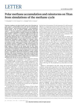
Figure 1 | Annual cycle of zonal-mean climate statistics in Titan GCM. The winter pole that is around 1 K colder than the summer pole. (Generally,
lower time axes start at the autumnal equinox (corresponding to November tropospheric temperatures in the simulation are within 1 K of Titan
1995); the upper axes indicate corresponding calendar years. Solid grey lines are observations; see Supplementary Fig. 2.) e, MSE per unit volume averaged
contours of absorbed solar radiation at the surface (contour interval between surface and 2-km altitude. MSE is the sum of gravitational potential
0.25 W m22), and dashed grey lines mark the northern summer solstice (NSS) energy and moist enthalpy, including the contribution of the latent heat of
and southern summer solstice (SSS). a, Methane surface-reservoir depth methane vapour26. f, Precipitation intensity (precipitation rate when it rains).
(colour scale truncated at 20 cm). b, Net evaporation (E 2 P) at the surface The precipitation intensity is the mean precipitation conditional on the
(colours, contour interval 0.1 mm day21, with 1 day 5 86,400 s) and column- precipitation rate being non-zero (exceeding 1023 mm day21). All fields are
integrated meridional methane flux (arrows, with the longest corresponding to averages over longitude and time (25 Titan yr) in the statistically steady state of a
a flux of 5.4 kg m21 s21). The methane flux is largely accomplished by the mean simulation with a total of 12 m liquid methane in the atmosphere–surface
meridional (Hadley) circulation; eddy fluxes are weaker by a factor of 3 or system. The statistically steady state was reached over a long (135 Titan yr) spin-
larger, and are strongest in the middle and low latitudes. c, Precipitation rate. up period. Although the GCM climate is statistically zonally symmetric, climate
d, Surface temperature. The surface temperatures are roughly consistent with statistics such as the methane surface-reservoir depth exhibit instantaneous
observations30, with similar equator–pole temperature contrasts and with a zonal asymmetries (‘lakes’), which can persist for several Titan years.
convection, even though they are warmer than the summer poles, caused by Saturn’s orbital eccentricity, which leads to a northern summer
because their maximum insolation is weaker, so their maximum (currently around aphelion) that is longer and cooler than the southern,
near-surface MSE is also lower (Fig. 1e). The result is the drying of and therefore allows more methane to be cold-trapped. Although the
lower latitudes and the accumulation of methane at the poles, similar maximum rate of net precipitation (Fig. 1b) is greatest in the warmer
to the results of previous models but without methane accumulation in southern summer, polar net precipitation integrated over a Titan year
mid-latitudes16 (see Supplementary Information for possible reasons (about 30 Earth years) is greatest in the north, primarily because its rainy
for this difference). season is longer. For example, averaged over the polar caps bounded
In the model’s low latitudes, rainstorms are rare but intense: that is, by the polar circles (63.3u N/S), the period during which absorbed
although low latitudes are dry and have smaller mean precipitation insolation exceeds 0.5 W m22 is 14% longer in the north than in the
rates than the poles (Fig. 1c), they have the largest precipitation intensity south. Annually integrated net precipitation is 0.86 m (38%) greater in
(Fig. 1f). Precipitation rates in the more intense storms are greater than the north; 0.76 m of this is attributable to increased precipitation, and
10 mm per (Earth) day, similar to rough estimates of the rates needed to 0.10 m to decreased evaporation. (The contribution of evaporation to
carve the observed fluvial surface features4,28. The precipitation intensity the hemispheric asymmetry is small because it scales with insolation,
is largest before and around the equinoxes, when the reversal of the which, in the annual mean, is equal in the north and south; this contra-
Hadley circulation (see Fig. 1b) is associated with dynamic instabilities. dicts a previous hypothesis that the hemispheric asymmetry is due to
These instabilities generate waves strong enough to trigger deep con- evaporation differences3.) In the model’s annual mean, the excess net
vection and intense rain if they advect relatively moist air from higher precipitation in polar regions is balanced by along-surface methane
latitudes over the warm low latitudes. This is in contrast to 2D and local transport towards mid-latitudes and subsequent evaporation, so sur-
models that suggest that intense precipitation does not occur in low face methane extends farther towards the equator in the north than in
latitudes16–18,20; however, it is consistent with the observations of intense the south (Fig. 1a). The same is true on Titan3. Thus, surface or sub-
and apparently precipitating low-latitude storms on Titan6,7. surface transport of methane is essential for maintaining a statistically
In the GCM as on Titan3, there is more surface methane in the steady state with non-zero net precipitation in polar regions and asym-
northern polar regions than in the southern (Fig. 1a). This asymmetry metries between the hemispheres; we expect that such transport occurs on
is a consistent feature, irrespective of initial conditions (for example, Titan. One reason that previous models16 did not produce hemispheric
whether methane is initially in the atmosphere or at the surface). It is asymmetries is that they were lacking a representation of this transport.
5 J A N U A RY 2 0 1 2 | VO L 4 8 1 | N AT U R E | 5 9
©2012 Macmillan Publishers Limited. All rights reserved

3. RESEARCH LETTER
30 Calendar year
Yr 9.1 32
a 2005 2010
VIMS Ground
Cloud frequency (%)
16 60° ISS
–0
Altitude (km)
20
.5
–1
8 30°
Latitude
–2
4 0°
10
32
2 –30°
-1
4 -16 –60° 16
Cloud frequency (%)
1
–60° –30° 0° 30° 60°
8
Latitude SSS 10 15
Figure 2 | Relationship between tropospheric cloudiness and atmospheric b 2000 2010 2020
4
circulation in southern summer in Titan GCM. Colours show the
tropospheric methane-cloud frequency and contours show the stream 60° 2
function of the mean meridional mass circulation, both at 9.1 yr past
autumnal equinox (corresponding to January 2005, the time of the Huygens
pffiffiffi 30°
landing on Titan). The contouring is logarithmic, with factors of 2 and 2 1
Latitude
between adjacent contour levels for cloud frequency and stream function, 0°
respectively. Solid stream-function contours for clockwise rotation, dashed
contours for anticlockwise rotation (contour levels at 6 221, 1, 2, 22, –30°
… 3 109 kg s21). The cloud frequency is the relative frequency of phase
changes of methane on the grid scale and in the convection scheme of the –60°
GCM. Moist convection and maxima in cloud frequency above the boundary
layer occur above the polar near-surface MSE maximum and above relatively
0 SSS 10 20 NSS
high surface temperatures in mid-latitudes (here, at around 30u S) in the
summer hemisphere. (Moist convection rarely occurs above the local surface- Time since autumnal equinox (yr)
temperature maximum in the winter hemisphere (here, at 15u–30u N), Figure 3 | Annual cycle of tropospheric methane-cloud frequency. a, Cloud
because this lies under the descending branch of the Hadley circulation, where frequency in GCM and cloud observations, focusing on the time period for which
the free troposphere is relatively dry.) detailed observations are available or will be available soon. The GCM cloud
frequency (colours) is a mass-weighted vertical average of the cloud frequency
(Fig. 2) in the troposphere between the surface and 32-km altitude. Brown circles,
Our GCM also reproduces the observed tropospheric methane- ground-based cloud observations13; magenta lines, Cassini VIMS observations14;
cloud distribution (Fig. 3). For the period with detailed observations light pink lines, Cassini ISS observations15. The bars across the top indicate the
(2001 onwards), the GCM reproduces the observed prevalence of time period over which the observations were made. (However, the coverage of
clouds in the southern hemisphere mid-latitudes and polar region; it VIMS and ISS observations is not continuous, so a lack of VIMS and ISS cloud
also reproduces the decreasing frequency of south-polar clouds since observations in the periods indicated by the bars does not necessarily mean clouds
2005 (Fig. 3a)6,13–15. For 2001 onwards, the GCM indicates a lack of were in fact absent.) Solid grey lines, contours of absorbed solar radiation at the
clouds in the northern hemisphere, consistent with observations of surface, as in Fig. 1. b, As in a, except over a complete Titan year, beginning at
autumnal equinox, and excluding observations.
Titan made with ground-based telescopes6,13 and the Cassini Visual
and Infrared Mapping Spectrometer (VIMS; ref. 14). Observations
with the Cassini Imaging Science Subsystem (ISS; ref. 15) indicate Received 4 August; accepted 20 October 2011.
more frequent northern-hemisphere clouds (Fig. 3a), but these seem 1. Stofan, E. et al. The lakes of Titan. Nature 445, 61–64 (2007).
to be lake-effect clouds: they are associated with stationary zonal in- 2. Hayes, A. et al. Hydrocarbon lakes on Titan: distribution and interaction with a
homogeneities in topography and the lake distribution29 that are not porous regolith. Geophys. Res. Lett. 35, L09204 (2008).
3. Aharonson, O. et al. An asymmetric distribution of lakes on Titan as a possible
captured in the GCM. The relative frequency of clouds in the GCM fits consequence of orbital forcing. Nature Geosci. 2, 851–854 (2009).
observations better than previous 2D models16–18. A 3D model that 4. Lebreton, J. et al. An overview of the descent and landing of the Huygens probe on
resolves waves and instabilities in the atmosphere is essential for repro- Titan. Nature 438, 758–764 (2005).
5. Lorenz, R. et al. The sand seas of Titan: Cassini RADAR observations of longitudinal
ducing the non-sinusoidal seasonal variations of cloudiness. dunes. Science 312, 724–727 (2006).
Deep convective clouds in the GCM form not only above the polar 6. Schaller, E. L., Roe, H. G., Schneider, T. & Brown, M. E. Storms in the tropics of Titan.
near-surface MSE maximum, but also in the summer-hemisphere Nature 460, 873–875 (2009).
7. Turtle, E. P. et al. Rapid and extensive surface changes near Titan’s equator:
mid-latitudes (Fig. 2). There they form above relatively high surface evidence of April showers. Science 331, 1414–1417 (2011).
temperatures (Fig. 1d), which destabilize the boundary layer with 8. Brown, M. E., Bouchez, A. H. & Griffith, C. A. Direct detection of variable tropospheric
respect to dry convection. This occasionally leads to moist convection clouds near Titan’s south pole. Nature 420, 795–797 (2002).
9. Porco, C. C. et al. Imaging of Titan from the Cassini spacecraft. Nature 434,
and mean ascent in the free troposphere (above shallow boundary- 159–168 (2005).
layer circulation cells), resulting in a secondary cloud-frequency 10. Griffith, C. A. et al. The evolution of Titan’s mid-latitude clouds. Science 310,
maximum above the boundary layer (Fig. 2). The surface reservoir 474–477 (2005).
underneath these clouds is depleted (less than 7 cm depth in the mean, 11. Roe, H. G., Bouchez, A. H., Trujillo, C. A., Schaller, E. L. & Brown, M. E. Discovery of
temperate latitude clouds on Titan. Astrophys. J. 618, L49–L52 (2005).
see Fig. 1a), consistent with the observed lack of lakes in mid-latitudes2. 12. Roe, H. G., Brown, M. E., Schaller, E. L., Bouchez, A. H. & Trujillo, C. A. Geographic
We predict that, with the reversal of the Hadley circulation in spring, control of Titan’s mid-latitude clouds. Science 310, 477–479 (2005).
north-polar clouds will emerge within about 2 yr, earlier than sug- 13. Schaller, E. L., Brown, M. E., Roe, H. G., Bouchez, A. H. & Trujillo, C. A. Dissipation of
Titan’s south polar clouds. Icarus 184, 517–523 (2006).
gested by other models17, and should be clearly observable for roughly 14. Brown, M. E., Roberts, J. E. & Schaller, E. L. Clouds on Titan during the Cassini prime
10 yr; around NSS, prominent cloudiness may extend into mid-lati- mission: A complete analysis of the VIMS data. Icarus 205, 571–580 (2010).
tudes (Fig. 3b). The validity of our predictions of seasonal changes will 15. Turtle, E. P. et al. Seasonal changes in Titan’s meteorology. Geophys. Res. Lett. 38,
L03203 (2011).
soon be testable as Titan’s northern-hemisphere spring proceeds into 16. Mitchell, J. The drying of Titan’s dunes: Titan’s methane hydrology and its impact
summer and new observations become available. on atmospheric circulation. J. Geophys. Res. 113, E08015 (2008).
6 0 | N AT U R E | VO L 4 8 1 | 5 J A N U A RY 2 0 1 2
©2012 Macmillan Publishers Limited. All rights reserved

4. LETTER RESEARCH
17. Mitchell, J. L., Pierrehumbert, R. T., Frierson, D. M. W. & Caballero, R. The dynamics 28. Perron, J. T. et al. Valley formation and methane precipitation rates on Titan.
behind Titan’s methane clouds. Proc. Natl Acad. Sci. USA 103, 18421–18426 J. Geophys. Res. 111, E11001 (2006).
(2006). 29. Brown, M. E. et al. Discovery of lake-effect clouds on Titan. Geophys. Res. Lett. 36,
18. Rannou, P., Montmessin, F., Hourdin, F. & Lebonnois, S. The latitudinal distribution L01103 (2009).
of clouds on Titan. Science 311, 201–205 (2006). 30. Jennings, D. E. et al. Titan’s surface brightness temperatures. Astrophys. J. 691,
19. Mitri, G., Showman, A. P., Lunine, J. I. & Lorenz, R. D. Hydrocarbon lakes on Titan. L103–L105 (2009).
Icarus 186, 385–394 (2007).
20. Griffith, C. A., McKay, C. P. & Ferri, F. Titan’s tropical storms in an evolving Supplementary Information is linked to the online version of the paper at
atmosphere. Astrophys. J. 687, L41–L44 (2008). www.nature.com/nature.
21. Flasar, F. M., Baines, K. H., Bird, M. K., Tokano, T. & West, R. A. Atmospheric
Acknowledgements We are grateful for support by a NASA Earth and Space Science
dynamics and meteorology. In Brown, R. H., Lebreton, J. P. & Waite, J. H. (eds) Titan
Fellowship and a David and Lucile Packard Fellowship. We thank I. Eisenman for code
from Cassini-Huygens Chap. 13, 323–352 (Springer, 2009).
for the insolation calculations, and O. Aharonson, A. Hayes and A. Soto for comments on
22. Schneider, T. The general circulation of the atmosphere. Annu. Rev. Earth Planet.
a draft. The simulations were done on the California Institute of Technology’s Division of
Sci. 34, 655–688 (2006).
Geological and Planetary Sciences Dell cluster.
23. Penteado, P. F., Griffith, C. A., Greathouse, T. K. & de Bergh, C. Measurements of
CH3D and CH4 in Titan from infrared spectroscopy. Astrophys. J. 629, L53–L56 Author Contributions T.S. and M.E.B. conceived the study; T.S., S.D.B.G. and E.L.S.
(2005). developed the GCM; E.L.S. and M.E.B. provided data; and T.S. and S.D.B.G. wrote the
24. Tokano, T. et al. Methane drizzle on Titan. Nature 442, 432–435 (2006). paper, with contributions and comments from all authors.
25. Hayes, A. et al. Transient surface liquid in Titan’s polar regions from Cassini. Icarus
211, 655–671 (2011). Author Information Reprints and permissions information is available at
26. Neelin, J. D. & Held, I. M. Modeling tropical convergence based on the moist static www.nature.com/reprints. The authors declare no competing financial interests.
energy budget. Mon. Weath. Rev. 115, 3–12 (1987). Readers are welcome to comment on the online version of this article at
27. Charney, J. G. A note on large-scale motions in the tropics. J. Atmos. Sci. 20, www.nature.com/nature. Correspondence and requests for materials should be
607–609 (1963). addressed to T.S. (tapio@caltech.edu).
5 J A N U A RY 2 0 1 2 | VO L 4 8 1 | N AT U R E | 6 1
©2012 Macmillan Publishers Limited. All rights reserved