Ch-5 Aggregate Supply-Slide Presentation.pdf

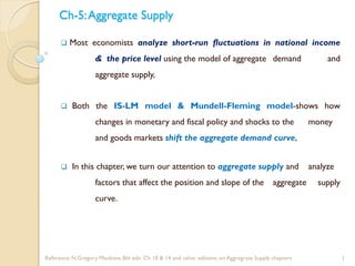
Ch-5:Aggregate Supply
 Most economists analyze short-run fluctuations in national income
& the price level using the model of aggregate demand and
aggregate supply,
 Both the IS-LM model & Mundell-Fleming model-shows how
changes in monetary and fiscal policy and shocks to the money
and goods markets shift the aggregate demand curve,
 In this chapter, we turn our attention to aggregate supply and analyze
factors that affect the position and slope of the aggregate supply
curve.
1
Reference: N.Gregory Mankiew, 8th edn. Ch 10 & 14 and other editions. on Aggregrate Supply chapters

5.2.The Classical Approach to Aggregate Supply Curve
 The classical approach to the aggregate supply analysis is based on
the long run aggregate supply which is represented by vertical
aggregate supply curve.
 This is b/s, the classical model describes how the economy behaves in
the long run, we derive the long-run aggregate supply curve from
the classical model,
 The classical aggregate supply curve is vertical, indicating that:
 the same amount of goods will be supplied whatever the price level i.e.
output does not depend on the price level (see fig 5.1),
 The classical supply curve is based on the assumption that the labor
market is in equilibrium with full employment of the labor force.
Reference: N.Gregory Mankiew, 8th edn. Ch 10 & 14 and other editions. on Aggregrate Supply chapters 2

o The vertical
aggregate supply
curve satisfies the
classical
dichotomy
between real &
nominal
variables, because
it implies that the
level of output(the
real value) is
independent of
the money
supply(nominal
value or money is
neutral in the long
run).
o This long run level
of output is called
the full
employment or
natural level of
output.
3
The Classical Approach to Aggregate Supply Curve…cond.
Fig 5.1: Classical Aggregate Supply Curve

 If the aggregate supply curve is vertical, then changes in aggregate demand affect prices but not output,
 For example, if the money supply falls, the aggregate demand curve shifts downwards, as in (fig 5.2),
 The economy moves from the old intersection of aggregate supply and aggregate demand, point A to
the new intersection, point B; but output remain constant.
 The shift in aggregate demand affects only prices.
The Classical Approach to Aggregate Supply Curve…cond.
Fig 5.2: Effect of Change in Aggregate Demand in the Classical Case

5.3: The Keynesian Approach to Aggregate Supply
 Unlike the classical, the Keynesian approach to aggregate supply
analysis is based in the short run,
 In the short run, some prices are sticky and, therefore, do not adjust to
changes in demand,
 Because of this price stickiness, short run aggregate supply curve is not
vertical,
 This is what we call the Keynesian Aggregate Supply Curve,
 In the extreme Keynesian case(when all prices are assumed to be sticky),
aggregate supply curve is horizontal; indicating that firms will supply
whatever amount of goods demanded at the existing price level (see figure
5-3 below).

The Keynesian Approach to Aggregate Supply…Cond.
Fig 5-3: Keynesian Aggregate Supply Curve

 The idea underlying the Keynesian
aggregate supply curve is that:
 because there is unemployment, firms can obtain
as much labor as they want at the current wage,
their average costs of production therefore are
assumed not to change as their output levels
change,
they are accordingly willing to supply as much
goods & services as is demanded at the existing
price level.

 The short run equilibrium of the economy is obtained at the intersection of the
aggregate demand curve and the horizontal short run aggregate supply curve,
 In this case, changes in aggregate demand either through fiscal policy or
monetary policy do affect the level of output in the economy.
 Suppose, for instance, the central bank reduces the money supply and thus the
aggregate demand curve shifts downward as in the fig 5.4,
 In the short run, prices are sticky, so the economy moves from point A to
point B,
 Output and employment fall below their natural levels, which means the
economy, is in recession,
 Over time, in response to the low demand, wages and prices fall,
 The gradual reduction in the price level moves the economy down ward along the
aggregate demand curve to pint C, which is the new long-run equilibrium.

Fig 5-4: Effect of Change in Aggregate Demand in the Keynesian

The BasicTheory of Aggregate Supply
 As already mentioned, economists usually analyze
short-run fluctuations in aggregate income and the
price level using the model of aggregate demand &
aggregate supply,
 In the previous sections we examined aggregate
demand in some detail using IS-LM model to shows
how changes in monetary and fiscal policies and
shocks to the money and goods market shift the
aggregate demand curve,
 In this section, we turn our attention to aggregate
supply and develop theories that explain the position
and slope of the aggregate supply curve.

 Under previous section, we took the extreme Keynesian case where
aggregate supply curve is horizontal, in which all prices are fixed,
 Our task in this section is to refine this understanding of short-run
aggregate supply,
 In fact, economists disagree about how best to explain aggregate supply,
 Hence, we look at four prominent models of short-run aggregate
supply curve.These are:
i) The Sticky-Price Model
ii) The Sticky-Wage Model
iii) The Worker-Misperception Model
iv) The Imperfect-Information Analysis

 In all models, some market imperfection (that is, some type
of friction) causes the output of the economy to deviate from
its natural level in the short-run,
 As a result, the short-run aggregate supply curve is
upward sloping,
shifts in the aggregate demand curve cause output to
fluctuate,
These temporary deviations of output from its
natural level represent the booms and busts of the
business cycle.

The BasicTheory of Aggregate Supply…cond.
 Each of these models:
 follows a different theoretical route, but
 both routes end up in the same place, i.e. a short-run aggregate supply
equation of the following form.
 Each of the models tells a different story about what lies behind this short-run
aggregate supply equation.
 In other words, each model highlights a particular reason why unexpected
movements in the price level are associated with fluctuations in aggregate
output.

The BasicTheory of Aggregate Supply-The Sticky Price Model
 The most widely accepted explanation for the upward-sloping
short-run aggregate supply curve is called the sticky-price model,
 This model emphasizes that firms do not instantly adjust the prices,
rather, they charge in response to changes in demand,
 Sometimes, prices are set by long-term contracts between firms and
customers,
Even without formal agreements, firms may hold prices steady
to avoid annoying their regular customers with frequent price
changes,
 Some prices are sticky because of the way markets are structured: once a
firm has printed and distributed its catalog or price list, it is costly to alter
prices.

The BasicTheory of Aggregate Supply-The Sticky Price Model…cond.
 To see how sticky prices can help explain an upward
sloping aggregate supply curve:
we first consider the pricing decisions of individual firms,
then
add together the decisions of many firms to explain the
behavior of the economy as a whole,
 Consider the pricing decision facing typical firm, the
firm’s desired price(p), depends on two macroeconomic
variables:
 The overall level of prices,
The level of aggregate income.

The overall level of prices(P)- a higher price
level implies that:
o the firm’s costs are higher,
oHence, the higher the overall price level, the more
the firm would like to charge for its product,
The level of aggregate income(Y):
oA higher level of income raises the demand for
the firm’s product,
Because marginal cost increases at higher
levels of production, the greater the demand,
the higher the firm’s desired price.

 We write the firm’s desired price as:
 This equation says that the desired price
(p) depends on:
 the overall level of prices (P), and
the level of aggregate output relative to the
natural rate,
o The parameter a (which is greater than
zero) measures how much the firm’s desired
price responds to the level of aggregate
output.

 Now assume that there are two types of firms:
 Some firm’s have flexible prices: they always set their prices
according to this equation.
Others have sticky price: they announce their prices in
advance based on what they expect economic conditions
to be.
 Firms with sticky price set price according to:

 We can use the pricing rules of the two groups of firms to derive the aggregate supply
equation,
 To do this, we find the overall price level in the economy, which is the weighted average
of the prices set by the two groups,
 If s is the fraction of firms with sticky prices and 1-s is the fraction with flexible prices,
 Then, the overall price level is:
 The first term is the price of the sticky-price firms weighted by their fraction in the
economy;
 the second term is the price of the flexible-price firms weighted by their fraction.
 Now subtract (1 - s)P from both sides of this equation to obtain

The two terms in this equation are explained as follows:
 When firms expect a high price level, they expect high costs.
 Those firms that fix prices in advance set their prices high,
 These high prices cause the other firms to set high prices also,
 Hence, a high expected price level EP leads to a high actual price level P,
 This effect does not depend on the fraction of firms with sticky prices.
 When output is high , the demand for goods is high.
 Those firms with flexible prices set their prices high, which leads to a high
price level,
 The effect of output on the price level depends on the fraction of firms
with sticky prices,
 The more firms that have sticky prices, the less the price level responds to
the level of economic activity.

 Hence, the overall price level depends on the
expected price level and on the level of
output.
 The sticky-price model says that the
deviation of output from the natural level is
positively associated with the deviation of the
price level from the expected price level.

The BasicTheory of Aggregate Supply-The StickyWage Model
o To explain why the short-run aggregate supply curve is upward
sloping, many economists stress the sluggish adjustment of nominal
wages,
o In many industries, nominal wages are set by long-term contracts, so
wages cannot adjust quickly when economic conditions change,
o Even in industries where there is no such formal contract, implicit
agreements between workers and firms may limit wage changes,
o Wages may also depend on social norms and notions of fairness that
evolve slowly,
o For these reasons, many economists believe that nominal wages are
sticky in the short-run.

The BasicTheory of Aggregate Supply-The Sticky Wage Model…cond.
 The sticky-wage model shows what a sticky nominal
wage implies for aggregate supply,
 To understand the model let us consider what happens to
the amount of output produced when the price level rises:
When nominal wage(W) is stuck, a rise in the price level
lowers the real wage (W/P), making labor cheaper,
The lower real wage induces firms to hire more labor because
labor demand is a function of the real wage (W/P),
The additional labor hired produces more output since output (Y)
is a function of employment of labor (L).

 This positive relationship between the price level and the amount of
output means that:
 the aggregate supply curve slopes upward during the time when nominal
wage cannot adjust,
 To develop this story of aggregate supply more formally:
 assume that workers & firms bargain over and agree on the nominal wage
before they know what the price level will be when their agreement
takes effect,
 Here, workers and firms have in mind a target real wage,
 The target may be the real wage that equilibrates labor supply and demand,
 More likely, the target real wage is higher than the equilibrium real wage
due to union power and the efficient wage consideration.

 The workers & firms set the nominal wage (W) based on:
 the target real wage (ω) and
their expectation of the price level (Ep).
 The nominal wage they set is therefore,
Nominal wage = Target real wage * expected price
W = ω * Ep
• After the nominal wage has been set and before labor
has been hired, firms learn the actual price level P.
• The real wage turns out to be
W/P = ω * (Ep/p)

 The above equation shows that the real wage deviates from its target if the
actual price level differs from the expected price level,
 When the actual price level is greater than expected, the real wage is less than
its target;
 When the actual price level is less than expected, the real wage is greater than
its target.
 The final assumption of the sticky-wage model is that employment is determined
by the quantity of labor that firms demand,
 We can describe the firm’s hiring decision by the following labor demand
function L=Ld(W/P) which states that the lower the real wage, the more labor
firms hire.
 If other inputs like capital(K) are assumed to be constant, then, output is determined
by the production function Y=F(L) which states that the more labor is hired,
the more output is produced.

Fig 5.5: The Sticky Wage and Aggregate Supply

 Panel (a) shows the labor demand curve,
 Because the nominal wage (W) is stuck, an increase in the price level
from P1 to P2 reduces real wage from W/P1 to W/P2,
 The lower real wage raises the quantity of labor demanded from
L1 to L2.
 Panel (b) shows the production function,
 An increase in the quantity of labor from L1 to L2 raises output from
Y1 toY2.
 Panel (c) on the other hand shows the aggregate supply curve that
summarizes the relationship between the price level and output,
An increase in the price level from P1 to P2 raises output
fromY1 toY2.

 Because the nominal wage is sticky in this model:
 an expected change in the price level moves the real wage away
from the target real wage,
and this change in the real wage influences the amounts of labor
hired and output produced,
The aggregate supply curve can be written as
 The equation states that output deviates from its natural rate
when the price level deviates from the expected price level.

The Basic Theory of Aggregate Supply-The Workers –Misperception Model…cond.
 The workers misperception model like that of the sticky-wage model focuses on the labor
market,
 It assumes wages are not sticky, but they are free to equilibrate supply and demand in the labor
market,
 Its key principle is that workers temporarily confuse real and nominal wages,
 The components of the model are labor demand (Ld) and labor supply (Ls) where:
 labor demand is a function of the actual real wage (W/P),
 labor supply is a function of the expected real wage (W/EP),
 Workers know W, but they do not know the overall price P,
 Hence, when they decide on how much to work, they consider the expected real wage(W/EP)
to be product of actual real wage(W/P) and misperception of workers regarding the level of
prices(P/EP).
W/EP=W/P*P/EP

The BasicTheory of Aggregate Supply-TheWorkers –Misperception Model…cond.
 Hence, labor supply (Ls)= Ls(W/P*P/EP ) that implies
labor supply is determined by the real wage and worker’s
misperceptions,
The implication for aggregate supply
 To see the implication of this model for aggregate supply
consider:
 an increase in the price level (P) and
 its impact on the labor market.
 When P rises there are two possible reactions in the
model
i) If workers anticipated the change, then:
 EP rises proportionately with P,
 And, hence there is no change in labor demand and labor supply.

The BasicTheory of Aggregate Supply-TheWorkers –Misperception Model…Cond.
ii) But, if workers are not aware of the price change, then:
 Then, expected price (EP) remains the same,
 Then,at every real wage:
 workers are willing to supply more labor because they believe that their real wage is higher than it
actually is,
 The increase in P/EP shifts the labor supply curve outward,
 The outward shift in labor supply lowers real wage and raise the level of employment,
 In essence, the increase in nominal wage caused by the rise in price level:
 leads workers to think that their real wage is higher, which induces them to supply more labor,
 But in actuality, the nominal wage rise by less than the price level,
 Here, firms are assumed to be better informed than workers and to recognize the fall in the real wage, so
they higher more labor and produce more output.
 In general, this model says that deviation of prices(P) from EP induce workers to alter their supply
of labor.

The BasicTheory of Aggregate Supply-The Imperfect-Information Model
 Another explanation for the upward slope of the short-run aggregate
supply curve is called the imperfect-information model,
 Unlike the previous model, this one assumes that markets clear i.e. all
prices are free to adjust to balance supply and demand,
 In this model, the short-run and long-run aggregate supply curves differ
because of temporary misperceptions about prices,
 The imperfect-information model assumes that each supplier in the
economy produces a single good and consumes many goods,
 Because the number of goods is so large, suppliers cannot observe all
prices at all times,
 They monitor closely the prices of what they produce but less closely the
prices of all the goods they consume.

The BasicTheory of Aggregate Supply-The Imperfect-Information Model…cond.
 Because of imperfect information, they sometimes confuse changes in the overall level of prices
with changes in relative prices,
 This confusion influences:
 decisions about how much to supply, and
 leads to a positive relationship between the price level and output in the short run,
 When the price level rises unexpectedly, all suppliers in the economy observe increases in the
prices of the goods they produce,
 They all infer, rationally but mistakenly, that the relative prices of the goods they produce have
risen,
 They work harder and produce more,
 To sum up, the imperfect-information model says that when actual prices exceed expected prices,
suppliers raise their output,
 The model implies an aggregate supply curve with the familiar form,
 Output deviates from the natural level when the price level deviates from the expected price level.

The BasicTheory of Aggregate Supply- Conclusion
 In this part, we have seen different models of aggregate supply,
 Each of these models uses to explain why the short run aggregate supply
curve is upward sloping,
 All models of aggregate supply:
 differ in their assumptions and emphasis,
 But all are similar in their implications for aggregate output are similar,
 All can be summarized by the equation
 This equation states that deviations of output from the natural level are
related to deviations of the price level from the expected price level.

 If the price level is higher than the expected
price level, output exceeds its natural level,
 If the price level is lower than the expected
price level, output falls short of its natural level,
 Figure 5.6, graph this equation:
Notice that the short-run aggregate supply curve is
drawn for a given expectation EP, and
that a change in EP would shift the curve.

Fig. 5.6: Short-Run Aggregate Supply Curve

 Now that we have a better understanding of aggregate supply, let's put
aggregate supply and aggregate demand back together,
 Figure 5.7 uses our aggregate supply equation to show how the economy
responds to an unexpected increase in aggregate demand attributable, say, to an
unexpected monetary expansion.
 In the short run,
 the equilibrium moves from point A to point B,
 The increase in aggregate demand raises the actual price level from P1 to P2,
 Because, people did not expect this increase in the price level:
 the expected price level remains at EP2, and
 output rises fromY1 toY2, which is above the natural level Y,
 Thus, the unexpected expansion in aggregate demand causes the
economy to boom.
 Yet, the boom does not last forever.

 In the long run,
 the expected price level rises to catch up with reality, causing the short-run aggregate supply
curve to shift upward,
 As the expected price level rises from EP2 to EP3, the equilibrium of the economy moves from point B to
point C,
 The actual price level rises from P2 to P3, and output falls fromY2 toY3.
 In other words, the economy returns to the natural level of output in the long run, but at a much higher price
level,
 This analysis demonstrates an important principle that holds for both models of aggregate
supply: long-run monetary neutrality and short-run monetary non-neutrality are perfectly
compatible.,
 Short-run non-neutrality is represented here by the movement from point A to point B, and
 long-run monetary neutrality is represented by the movement from point A to point C,
 We reconcile the short-run and long-run effects of money by emphasizing the adjustment of
expectations about the price level.
39

Fig 5.7: Effect of Shift in Aggregate Demand Curve on Aggregate Supply Curve

Ch-5 Aggregate Supply-Slide Presentation.pdf

Recommandé

Recommandé

Contenu connexe

Similaire à Ch-5 Aggregate Supply-Slide Presentation.pdf

Similaire à Ch-5 Aggregate Supply-Slide Presentation.pdf (20)

Dernier

Dernier (20)

Ch-5 Aggregate Supply-Slide Presentation.pdf