1. UNIT 9 COST CONCEPTS AND
ANALYSIS II
Objectives
After studying this unit, you should be able to:
analyse the behaviour of costs both in short run and long run;
comprehend the different sources of economies of scale;
apply cost concepts and analysis in managerial decision-making.
Structure
9.1 Introduction
9.2 Short-run Cost Functions
9.3 Long-run Cost Functions
9.4 Economies and Diseconomies of Scale
9.5 Economies of Scope
9.6 Application of Cost Analysis
9.7 Summary
9.8 Self-Assessment Questions
9.9 Further Readings
9.1 INTRODUCTION
In unit 8, you have learnt different cost concepts used by managers in decision-
making process, the relationship between these concepts, and the distinction
between accounting costs and economic costs. We will continue the analysis
of costs in this unit also.
To make wise decisions concerning how much to produce and what prices to
charge, a manager must understand the relationship between firm’s output rate
and its costs. In this unit, we learn to analyse in detail the nature of this
relationship, both in short run and long run.
9.2 SHORT-RUN COST FUNCTIONS
In Unit 8 we have distinguished between the short run and the long run. We
also distinguished between fixed costs and variable costs. The distinction
between fixed and variable costs is of great significance to the business
manager. Variable costs are those costs, which the business manager can
control or alter in the short run by changing levels of production. On the other
hand, fixed costs are clearly beyond business manager’s control, such costs are
incurred in the short run and must be paid regardless of output.
Total Costs
Three concepts of total cost in the short run must be considered: total fixed
cost (TFC), total variable cost (TVC), and total cost (TC). Total fixed costs
are the total costs per period of time incurred by the firm for fixed inputs.
Since the amount of the fixed inputs is fixed, the total fixed cost will be the
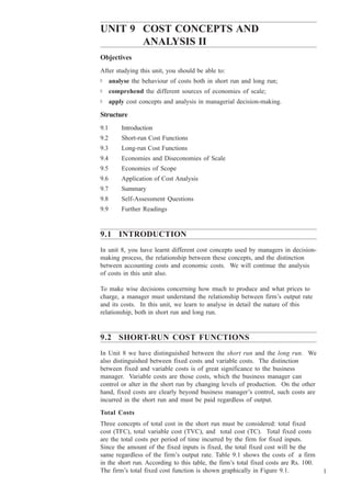
same regardless of the firm’s output rate. Table 9.1 shows the costs of a firm
in the short run. According to this table, the firm’s total fixed costs are Rs. 100.
The firm’s total fixed cost function is shown graphically in Figure 9.1. 1

2. Production and Table 9.1: A Firm’s Short Run Costs (in Rs.) Cost Concepts and
Cost Analysis Analysis II
Q TFC TVC TC MC AFC AVC ATC
0 100 0 100
1 100 50 150 50 100.0 50 150
2 100 90 190 40 50.0 45 95.0
3 100 120 220 30 33.3 40 73.3
4 100 140 240 20 25.0 35 60.0
5 100 150 250 10 20.0 30 50.0
6 100 156 256 6 16.7 26 42.7
7 100 175 275 19 14.3 25 39.3
8 100 208 308 33 12.5 26 38.5
9 100 270 370 62 11.1 30 41.1
10 100 350 450 80 10.0 35 45.0
Figure 9.1: Total Cost Curves
500
450
400
350
TC, TFC, TVC
300
250
200
150
100
50
0
0 1 2 3 4 5 6 7 8 9 10
Output (Q)
Total variable costs are the total costs incurred by the firm for variable inputs.
To obtain total variable cost we must know the price of the variable inputs.
Suppose if we have two variable inputs viz. labour (V1) and raw material (V2)
and the corresponding prices of these inputs are P1 and P2, then the total
variable cost (TVC) = P1 * V1 + P2 * V2. They go up as the firm’s output
rises, since higher output rates require higher variable input rates, which mean
bigger variable costs. The firm’s total variable cost function corresponding to
the data given in Table 9.1 is shown graphically in Figure 9.1.
Finally, total costs are the sum of total fixed costs and total variable costs. To
2 derive the total cost column in Table 9.1, add total fixed cost and total variable

3. cost at each output. The firm’s total cost function corresponding to the data
given in Table 9.1 is shown graphically in Figure 9.1. Since total fixed costs
are constant, the total fixed cost curve is simply a horizontal line at Rs.100.
And because total cost is the sum of total variable costs and total fixed costs,
the total cost curve has the same shape as the total variable cost curve but lies
above it by a vertical distance of Rs. 100.
Corresponding to our discussion above we can define the following for the
short run:
TC = TFC + TVC
Where,
TC = total cost
TFC = total fixed costs
TVC = total variable costs
Average Fixed Costs
While the total cost functions are of great importance, managers must be
interested as well in the average cost functions and the marginal cost function
as well. There are three average cost concepts corresponding to the three total
cost concepts. These are average fixed cost (AFC), average variable cost
(AVC), and average total cost (ATC). Figure 9.2 show typical average fixed
cost function graphically. Average fixed cost is the total fixed cost divided by
output. Average fixed cost declines as output (Q) increases. Thus we can
write average fixed cost as:
AFC = TFC/Q
Figure 9.2: Short Run Average and Marginal Cost Curves
MC
ATC
AVC
ATC, AVC, AFC, MC
AFC
O (Q)
Output (Q)
Average Variable Costs
Average variable cost is the total variable cost divided by output. Figure 9.2
shows the average variable cost function graphically. At first, output increases
resulting in decrease in average variable cost, but beyond a point, they result in
higher average variable cost.
TVC
AVC = ———
Q
3

4. Production and
Where, Cost Concepts and
Cost Analysis Analysis II
Q = output
TVC = total variable costs
AVC = average variable costs
Average Total Cost
Average total cost (ATC) is the sum of the average fixed cost and average
variable cost. In other words, ATC is total cost divided by output. Thus,
TC
ATC = AFC + AVC = ——
Q
Figure 9.2 shows the average total cost function graphically. Since ATC is sum
of the AFC and AVC, ATC curve always exceeds AVC curve. Also, since
AFC falls as output increases, AVC and ATC get closer as output rises. Note
that ATC curve is nearer the AFC curve at initial levels of output, but is nearer
the AVC curve at later levels of output. This indicates that at lower levels of
output fixed costs are more important part of the total cost, while at higher
levels of output the variable element of cost becomes more important.
Marginal Cost
Marginal cost (MC) is the addition to either total cost or total variable cost
resulting from the addition of one unit of output. Thus,
W TC W TVC
MC = ——— = ———
WQ WQ
Where,
MC = marginal cost
WQ = change in output
W TC = change in total cost due to change in output
WTVC = change in total variable cost due to change in output
The two definitions are the same because, when output increases, total cost
increases by the same amount as the increase in total variable cost (since fixed
cost remains constant). Figure 9.2 shows the marginal cost function
graphically. At low output levels, marginal cost may decrease with increase in
output, but after reaching a minimum, it goes up with further increase in output.
The reason for this behaviour is found in diminishing marginal returns.
The marginal cost concept is very crucial from the manager’s point of view.
Marginal cost is a strategic concept because it designates those costs over
which the firm has the most direct control. More specifically, MC indicates
those costs which are incurred in the production of the last unit of output and
therefore, also the cost which can be “saved” by reducing total output by the
last unit. Average cost figures do not provide this information. A firm’s
decisions as to what output level to produce is largely influenced by its marginal
cost. When coupled with marginal revenue, which indicates the change in
revenue from one more or one less unit of output, marginal cost allows a firm
to determine whether it is profitable to expand or contract its level of
production.
Relationship between Marginal Cost and Average Costs
The relationships between the various average and marginal cost curves are
illustrated in Figure 9.2. The figure shows typical AFC, AVC, ATC, and MC
curves but is not drawn to scale for the data given in Table 9.1. The MC cuts
4

5. both AVC and ATC at their minimum. When both the MC and AVC are
falling, AVC will fall at a slower rate. When both the MC and AVC are rising,
MC will rise at a faster rate. As a result, MC will attain its minimum before
the AVC. In other words, when MC is less than AVC, the AVC will fall, and
when MC exceeds AVC, AVC will rise. This means that as long as MC lies
below AVC, the latter will fall and where MC is above AVC, AVC will rise.
Therefore, at the point of intersection where MC = AVC, AVC has just ceased
to fall and attained its minimum, but has not yet begun to rise. Similarly, the
MC curve cuts the ATC curve at the latter’s minimum point. This is because
MC can be defined as the addition either to TC or TVC resulting from one
more unit of output. However, no such relationship exists between MC and
AFC, because the two are not related; MC by definition includes only those
costs which change with output, and FC by definition is independent of
output.
Relationship between Average Product and Marginal Product, and
Average Variable Cost and Marginal Cost
There is a straightforward relationship between factor productivity and output
costs. To see this, let us consider a single variable factor L say labour. All
other inputs are fixed. AP and MP will denote the average and marginal
products of labour, respectively. If W is the wage rate and L is the quantity
of labour, then
TVC = W * L
Hence, if Q is the output,
TVC ⎧ L ⎫
AVC = = W ⎨ ⎬
Q ⎩ Q ⎭
Consequently, since Q/W is the average product (AP), AVC = W/AP
Also, WTVC = W * WL (W does not change and is assumed to be given.).
Dividing by WQ we get
∆TVC ⎧ ∆L ⎫
MC = = W ⎨ ⎬
∆Q ⎩ ∆Q ⎭
But, marginal product (MP) = WQ/ W L. Hence, MC = W/MP
Figure 9.3 shows the relationship between average product and marginal
product, and average variable cost and marginal cost. The relationship AVC =
W/AP shows that AVC is at a minimum when AP is at maximum. Similarly,
the relationship MC = W/MP shows that MC is at a minimum when MP is at
a maximum. Also, when AP is at a maximum, AP = MP. Hence, when AVC
is at a minimum, AVC = MC. It is clearly shown that when MP is rising, MC
is falling. And when MP is falling, MC is rising.
The relevant costs to be considered for decision-making will differ from one
situation to the other depending on the problem faced by the manager. In
general, the TC concept is quite useful in finding out the breakeven quantity of
output. The TC concept is also used to find out whether firm is making profits
or not. The AC concept is important for calculating the per unit profit of a
business firm. The MC concept is essential to decide whether a firm should
expand its production or not.
5

6. Production and Figure 9.3: Relationship between AP and MP, AVC and MC Cost Concepts and
Cost Analysis Analysis II
AP, MP
AP
L1 L2 Output (Q)
MP
MC
AVC
AVC, MC
Q1 Q2 Labour Input
Activity 1
1. Fill in the blanks in the Table below:
Q TFC TVC TC AFC AVC ATC MC
1. 50 55
2. 50 8 25
3. 50 60.5
4. 13
5. 50 65
6. 50 18 3 11.3 3
7. 50 72.5
8. 50 28
9. 86
10 50 45 5 9.5 9
11. 50 54.5 4.5 9.5 9.5
12. 50 65.2
13. 50 130
6

7. 14. 50 99.1
15. 50 174.75
16. 50 162
17. 50 259.25
18. 269.5
19. 50 399
20. 50 450 2.5 22.5 25 101
Note: Output Q is measured in ’000 units
All costs are measured in Rs. ’000
2. Suppose that a firm is currently employing 20 workers, the only variable
input, at wage rate of Rs. 60. The average product of labour is 30, the last
worker added 12 units to total output, and total fixed cost is Rs. 3600.
a. What is the marginal cost? ......................................................................
b. What is the average variable cost? ........................................................
c. How much output is being produced? ....................................................
d. What is the average total cost? .............................................................
e. Is average variable cost increasing, constant, or decreasing? What about
average total cost? .................................................................................
3. Suppose average variable cost is constant over a range of output. What is
marginal cost over this range? What is happening to average total cost over
this range?
.....................................................................................................................
.....................................................................................................................
.....................................................................................................................
.....................................................................................................................
9.3 LONG-RUN COST FUNCTIONS
In the long run, all inputs are variable, and a firm can have a number of
alternative plant sizes and levels of output that it wants. There are no fixed
cost functions (total or average) in the long run, since no inputs are fixed. A
useful way of looking at the long run is to consider it a planning horizon. The
long run cost curve is also called planning curve because it helps the firm in
future decision making process.
AVC
Figure 9.4: Short-Run and Long-Run Average Cost Curves
SRAC3
C2 SRAC4
SRAC1 SRAC2
C1
a
Q1 Q2 Q3 Q4 Output (Q)
7

8. Production and
The long run cost output relationship can be shown with the help of a long run Cost Concepts and
Cost Analysis Analysis II
cost curve. The long run average cost curve (LRAC) is derived from short
run average cost curves (SRAC). Let us illustrate this with the help of a
simple example. A firm faces a choice of production with three different
plant sizes viz. plant size-1 (small size), plant size-2 (medium size), plant size-3
(large size), and plant size-4 (very large size). The short run average cost
functions shown in Figure 9.4 (SRAC1, SRAC2, SRAC3, and SRAC4) are
associated with each of these plants discrete scale of operation. The long run
average cost function for this firm is defined by the minimum average cost of
each level of output. For example, output rate Q1 could be produced by the
plant size-1 at an average cost of C1 or by plant size-2 at a cost of C2.
Clearly, the average cost is lower for plant size-1, and thus point a is one point
on the long run average cost curve. By repeating this process for various
rates of output, the long run average cost is determined. For output rates of
zero to Q2 plant size-1is the most efficient and that part of SRAC1 is part of
the long run cost function. For output rates of Q2 to Q3 plant size-2 is the
most efficient, and for output rates Q3 to Q4, plant size-3 is the most efficient.
The scallop-shaped curve shown in boldface in Figure 9.4 is the long run
average cost curve for this firm. This boldfaced curve is called an envelope
curve (as it envelopes short run average cost curves). Firms plan to be on this
envelope curve in the long run. Consider a firm currently operating plant
size-2 and producing Q1 units at a cost of C2 per unit. If output is expected to
remain at Q1, the firm will plan to adjust to plant size-1, thus reducing average
cost to C1.
Most firms will have many alternative plant sizes to choose from, and there is
a short run average cost curve corresponding to each. A few of the short run
average cost curves for these plants are shown in Figure 9.5, although many
more may exist. Only one point of a very small arc of each short run cost
curve will lie on the long run average cost function. Thus long run average
cost curve can be shown as the smooth U-shaped curve. Corresponding to
this long run average cost curve is a long run marginal cost (LRMC) curve,
which intersects LRAC at its minimum point a, which is also the minimum point
of short run average cost curve 4 (SRAC4). Thus, at a point a and only at a
point a, the following unique result occurs:
SRAC = SRMC when LRAC = LRMC
Figure 9.5: Short-Run and Long-Run Average Cost and Marginal Cost Curves
SRAC1
AVC, MC
SRAC7
SRAC2
SRAC6
SRAC3 SRAC4
SRAC5
C1
C2
a
LRMC
Q* Output (Q)
8

9. The long run cost curve serves as a long run planning mechanism for the firm.
It shows the least per unit cost at any output can be produced after the firm
has had time to make all appropriate adjustments in its plant size. For
example, suppose that the firm is operating on short run average cost curve
SRAC3 as shown in Figure 9.5, and the firm is currently producing an output
of Q*. By using SRAC3, it is seen that the firm’s average cost is C2.
Clearly, if projections of future demand indicate that the firm could expect to
continue selling Q* units per period at the market price, profit could be
increased significantly by increasing the scale of plant to the size associated
with short run average cost curve SRAC4. With this plant, average cost for an
output rate of Q* would be C2 and the firm’s profit per unit would increase by
C2 – C1. Thus, total profit would increase by (C2 – C1) * Q*.
The U-shape of the LRAC curve reflects the laws of returns to scale.
According to these laws, the cost per unit of production decreases as plant size
increases due to the economies of scale, which the larger plant sizes make
possible. But the economies of scale exist only up to a certain size of plant,
known as the optimum plant size where all possible economies of scale are
fully exploited. Beyond the optimum plant size, diseconomies of scale arise due
to managerial inefficiencies. As plant size increases beyond a limit, the control,
the feedback of information at different levels and decision-making process
becomes less efficient. This makes the LRAC curve turn upwards. Given the
LRAC in Figure 9.5, we can say that there are increasing returns to scale up
to Q* and decreasing returns to scale beyond Q*. Therefore, the point Q* is
the point of optimum output and the corresponding plant size-4 is the optimum
plant size.
If you have long run average cost of producing a given output, you can readily
derive the long run total cost (LRTC) of the output, since the long run total
cost is simply the product of long run average cost and output. Thus, LRTC =
LRAC * Q.
Figure 9.6 shows the relationship between long run total cost and output.
Given the long run total cost function you can readily derive the long run
marginal cost function, which shows the relationship between output and the
cost resulting from the production of the last unit of output, if the firm has time
to make the optimal changes in the quantities of all inputs used.
Figure 9.6: Long Run Total Cost Function
Long Run Total Cost (LRTC)
Long Run Total Cost
O Output (Q)
(Q)
9

10. Production and
Activity 2 Cost Concepts and
Cost Analysis Analysis II
1. Explain why short run marginal cost is greater than long run marginal cost
beyond the point at which they are equal?
.....................................................................................................................
.....................................................................................................................
.....................................................................................................................
.....................................................................................................................
.....................................................................................................................
2. Explain why short run average cost can never be less than long run average
cost?
.....................................................................................................................
.....................................................................................................................
.....................................................................................................................
.....................................................................................................................
.....................................................................................................................
3. Why are all costs variable in the long run?
.....................................................................................................................
.....................................................................................................................
.....................................................................................................................
.....................................................................................................................
.....................................................................................................................
4. Why is the long run average cost curve called an “envelope curve”?
Why cannot the long run marginal cost curve be an envelope as well?
.....................................................................................................................
.....................................................................................................................
.....................................................................................................................
.....................................................................................................................
.....................................................................................................................
5. What do you understand by ” cost -efficiency”? Draw a long run cost
diagram and explain.
.....................................................................................................................
.....................................................................................................................
.....................................................................................................................
.....................................................................................................................
.....................................................................................................................
.....................................................................................................................
6. Economists frequently say that the firm plans in the long run and operates in
the short run. Explain.
.....................................................................................................................
.....................................................................................................................
.....................................................................................................................
.....................................................................................................................
.....................................................................................................................
.....................................................................................................................
10

11. 9.4 ECONOMIES AND DISECONOMIES OF SCALE
We have seen in the preceding section that larger plant will lead to lower
average cost in the long run. However, beyond some point, successively larger
plants will mean higher average costs. Exactly, why is the long run average
cost (LRAC) curve U-shaped? What determines the shape of LARC curve?
This point needs further explanation.
It must be emphasized here that the law of diminishing returns is not applicable
in the long run as all inputs are variable. Also, we assume that resource
prices are constant. What then, is our explanation? The U-shaped LRAC
curve is explainable in terms of what economists call economies of scale and
diseconomies of scale.
Economies and diseconomies of scale are concerned with behaviour of average
cost curve as the plant size is increased. If LRAC declines as output
increases, then we say that the firm enjoys economies of scale. If, instead, the
LRAC increases as output increases, then we have diseconomies of scale.
Finally, if LRAC is constant as output increases, then we have constant returns
to scale implying we have neither economies of scale nor diseconomies of
scale.
Economies of scale explain the down sloping part of the LRAC curve. As the
size of the plant increases, LRAC typically declines over some range of output
for a number of reasons. The most important is that, as the scale of output is
expanded, there is greater potential for specialization of productive factors.
This is most notable with regard to labour but may apply to other factors as
well. Other factors contributing to declining LRAC include ability to use
more advanced technologies and more efficient capital equipment; managerial
specialization; opportunity to take advantage of lower costs (discounts) for
some inputs by purchasing larger quantities; effective utilization of by products,
etc.
But, after sometime, expansion of a firm’s output may give rise to
diseconomies, and therefore, higher average costs. Further expansion of output
beyond a reasonable level may lead to problems of over crowding of labour,
managerial inefficiencies, etc., pushing up the average costs.
In this section, we examined the shape of the LRAC curve. In other words,
we have analysed the relationship between firm’s output and its long run
average costs. The economies of scale and diseconomies of scale are some
times called as internal economies of scale and internal diseconomies of
scale respectively. This is because the changes in long run average costs
result solely from the individual firm’s adjustment of its output. On the other
hand, there may exist external economies of scale. The external economies
also help in cutting down production costs. With the expansion of an industry,
certain specialized firms also come up for working up the by-products and
waste materials. Similarly, with the expansion of the industry, certain
specialized units may come up for supplying raw material, tools, etc., to the
firms in the industry. Moreover, they can combine together to undertake
research etc., whose benefit will accrue to all firms in the industry. Thus, a
firm benefits from expansion of the industry as a whole. These benefits are
external to the firm, in the sense that these have arisen not because of any
effort on the part of the firm but have accrued to it due to expansion of
industry as a whole. All these external economies help in reducing production
costs.
11

12. Production and
Economies of scale are often measured in terms of cost-output elasticity, Ec. Cost Concepts and
Cost Analysis Analysis II
Ec is the percentage change in the average cost of production resulting from a
one percent increase in output:
E c = (WTC/TC) / (WQ/Q) = (WTC/ WQ) / (TC/Q) = MC/AC
Clearly, Ec is equal to one when marginal and average costs are equal. This
means costs increase proportionately with output, and there are neither
economies nor diseconomies of scale. When there are economies of scale
MC will be less than AC (both are declining) and Ec is less than one. Finally,
when there are diseconomies of scale, MC is greater than AC, and Ec is
greater than one.
Activity 3
1. Distinguish between internal and external economies of scale. Give
examples.
.....................................................................................................................
.....................................................................................................................
.....................................................................................................................
.....................................................................................................................
.....................................................................................................................
9.5 ECONOMIES OF SCOPE
According to the concept of economies of scale, cost advantages follow the
increase in volume of production or what is called the scale of output. On the
other hand, according to the concept of economies of scope, such cost
advantages may follow from a variety of output. For example, many firms
produce more than one product and the products are closely related to one
another — an automobile company produces scooters and cars, and a university
produces teaching and research. A firm is likely to enjoy production or cost
advantages when it produces two or more products. These advantages could
result from the joint use of inputs or production facilities, joint marketing
programs, or possibly the cost savings of a common administration. Examples
of joint products are mutton and wool, eggs and chicken, fertilizer, etc.
Therefore, economies of scope exist when the cost of producing two (or more)
products jointly is less than the cost of producing a single product. To measure
the degree to which there are economies of scope, we should know what
percentage of the cost of production is saved when two (or more) products are
produced jointly rather than individually. The following equation gives the
degree of economies of scope (SC) that measures the savings in cost:
C (Q1) + C (Q2) – C (Q1 + Q2)
SC = —————————————
C (Q 1 + Q2)
Here, C (Q1) represents the cost of producing output Q1, C (Q2) the cost of
producing output Q2, and C (Q1, Q2) the joint cost of producing both outputs
(Q 1 + Q 2).
For example, a firm produces 10000 TV sets and 5000 Radio sets per year at
a cost of Rs.8.40 crores, and another firm produces 10000 TV sets only, then
the cost would be Rs.10.00 crores, and if it produced 5000 Radio sets only,
12 then the cost would be Rs. 0.50 crores. In this case, the cost of producing

13. both the TV and Radio sets is less than the total cost of producing each
separately. Thus, there are economies of scope. Thus,
10.00 + 0.50 – 8.40
SC = ————————— = 0.25
8.40
Which means that there is a 25% saving of cost by going for joint production.
With economies of scope, the joint cost is less than the sum of the individual
costs, so that SC is greater than 0. With diseconomies of scope, SC is
negative. In general, the larger the value of SC, the greater is the economies
of scope.
Activity 4
1. Distinguish between economies of scale and economies of scope using
examples.
.....................................................................................................................
.....................................................................................................................
.....................................................................................................................
.....................................................................................................................
9.6 APPLICATION OF COST ANALYSIS
In the previous sections of this unit we discussed total, marginal, and average
cost curves for both short run and long run. The relationships between these
cost curves have a very wide range of applications for managerial use. Here
we will discuss a few applications of these concepts.
Determining Optimum Output Level
Earlier we have seen that the optimum output level is the point where average
cost is minimum. In other words, the optimum output level is the point where
average cost equals marginal cost. Consider the following example.
TC = 128 + 6Q +2Q2
This is a short run total cost function since there is a fixed cost (TFC = 128).
128
AC = (TC/Q) = —— + 6 + 2Q
Q
d (AC) 128
———— = – —— + 2 = 0
dQ Q2
2Q2 = 128
Q2 = 64
Q = 8
or
d (TC)
MC = ——— = 6 + 4Q = 0
dQ
13

14. Production and
setting AC = MC Cost Concepts and
Cost Analysis Analysis II
128
—— + 6 + 2Q = 6 + 4Q
Q
128
——— – 2Q = 0
Q
2Q2 = 128
Q = 8
Thus Q = 8 and is the optimum level of output in the short run.
Breakeven Output Level
An analytical tool frequently employed by managerial economists is the
breakeven chart, an important application of cost functions. The breakeven
chart illustrates at what level of output in the short run, the total revenue just
covers total costs. Generally, a breakeven chart assumes that the firm’s
average variable costs are constant in the relevant output range; hence, the
firm’s total cost function is assumed to be a straight line. Since variable cost is
constant, the marginal cost is also constant and equals to average variable cost.
Figure 9.7 shows the breakeven chart of a firm. Here, it is assumed that the
price of the product will not be affected by the quantity of sales. Therefore,
the total revenue is proportional to output. Consequently, the total revenue
curve is a straight line through the origin. The firm’s fixed cost is Rs. 500,
variable cost per unit is Rs. 4 and the unit sales price of output is Rs. 5. The
breakeven chart, which combines the total cost function and the total revenue
curve, shows profit or loss resulting from each sales level. For example, Figure
9.7 shows that if the firm sells 200 units of output it will make a loss of
Rs. 300. The chart also shows the breakeven point, the output level that must
be reached if the firm is to avoid losses. It can be seen from the figure, the
breakeven point is 500 units of output. Beyond 500 units of output the firm
makes profit.
Figure 9.7: Breakeven Chart
5000
4500 Total revenue
4000
Profit
Total Cost/Total Revenue
3500
Total cost
3000
2500
2000
1500 Loss
1000
500
0
0 100 200 300 400 500 600 700 800 900 1000
14 Output (Q)

15. Breakeven charts are used extensively for managerial decision process. Under
right conditions, breakeven charts can produce useful projections of the effect
of the output rate on costs, revenue and profits. For example, a firm may use
breakeven chart to determine the effect of projected decline in sales or profits.
On the other hand, the firm may use it to determine how many units of a
particular product it must sell in order to breakeven or to make a particular
level of profit. However, breakeven charts must be used with caution, since
the assumptions underlying them, sometimes, may not be appropriate. If the
product price is highly variable or if costs are difficult to predict, the estimated
total cost function and revenue curves may be subject to these errors.
We can analyse the breakeven output with familiar algebraic equations.
TR = P * Q
TC = FC + AVC * Q
At breakeven point, TR = TC
P * Q = FC + AVC * Q
FC Total fixed costs
Q = ———— = ——————————————
P – AVC Price – Variable Cost per unit
Here Q stands for breakeven volume of output. Multiplying Q with price (P)
we get the breakeven value of output. In the case of our example given in
Figure 9.7, FC = Rs. 500, P = Rs. 5 and AVC = Rs. 4. Consequently,
500 500
Q = ——— = ——— = 500
5 – 4 1
Therefore, the breakeven output (Q) will be 500 units. Similarly, the breakeven
output value will be Rs.2500 (P * Q = Rs. 5 * 500).
Profit Contribution Analysis
In making short run decisions, firms often find it useful to carry out profit
contribution analysis. The profit contribution is the difference between price
and average variable cost (P – AVC). That is, revenue on the sale of a unit
of output after variable costs are covered represents a contribution towards
profit. In our example since price is Rs.5 and average variable cost is Rs.4, the
profit contribution per unit of output will be Rs.1 (Rs.5 – Rs.4). At low
rates of output the firm may be losing money because fixed costs have not yet
been covered by the profit contribution. Thus, at these low rates of output,
profit contribution is used to cover fixed costs. After fixed costs are covered,
the firm will be earning a profit.
A manager wants to know the output rate necessary to cover all fixed costs
and to earn a ‘required’ profit (pR). Assume that both price and AVC are
constant. Profit is equal to revenue less the sum of total variable costs and
fixed costs. Thus
p R = P * Q – [(Q * AVC) + FC]
Solving this equation for Q gives a relation that can be used to determine the
rate of output necessary to generate a specified rate of profit. Thus
15

16. Production and FC + p R Cost Concepts and
Cost Analysis Analysis II
Q = —————
P – AVC
To illustrate how profit contribution analysis can be used, suppose that the firm
in our example (where FC = Rs. 500, P = Rs. 4 and AVC = Rs. 2.50) wants
to determine how many units of output it will have to produce and sell to earn
a profit of Rs.10, 000. To generate this profit, an output rate of 10,500 units is
required; that is,
Rs.500 + Rs.10,000
Q = ————————– = 10,500
Rs.5 – Rs.4
Operating Leverage
Managers must make comparisons among alternative systems of production.
Should one type of plant be replaced by another? Breakeven analysis can be
extended to help make such comparisons more effective. Consider the degree
of operating leverage (Ep), which is defined as the percentage change in
profit resulting from a 1% change in the number of units of product sold. Thus
% change in profit
Ep = ———————————
% change in output sold
(W p / p ) W p Q dp Q
= ——–———— = ——— * ——— or —— * ——
(W Q/Q) WQ p dQ p
If the price of output is constant regardless of the rate of output, the change in
degree of operating leverage depends on three variables: the rate of output, the
level of fixed costs, and variable cost per unit of output. This can be seen by
substituting the above equation for profit with
p = P * Q – (AVC) * Q – TFC
and change in profit W p = P * WQ – (AVC) * WQ
Therefore, the degree of operating leverage will be
[P * WQ – (AVC) * WQ]/[P * Q – (AVC) * Q – TFC]
Ep = —————————————————————————
W Q/Q
On simplification
Q(P – AVC)
Ep = ————————
Q(P – AVC) – TFC
Example: Consider three firms I, II and III having the following fixed costs,
average variable costs and price of the product.
16

17. Firm Fixed Cost (Rs.) Average variable Price of the product
Cost (Rs.) (Rs.)
Firm-I 1,00,000 2 5
Firm-II 60,000 3 5
Firm-III 26,650 4 5
Firm-I has more fixed cost than firm-II, and firm-III. However, Firm-I has
less average costs than firm-II, and firm-III. Essentially, firm-I has substituted
capital (fixed costs) for labour and materials (variable costs) with the
introduction more mechanized machines. On the other hand, firm-III has less
fixed costs and more average variable costs when compared to other two
plants because firm-III has less mechanized machines. The firm-II occupies
middle position in terms of fixed costs and average variable costs.
In comparing these plants, we use the degree of operating leverage. Suppose
for all the three plants Q = 40,000
40000 (5 – 2)
For firm-I, Ep = ———————————— = 6
40000 (5 – 2) – 100000
40000 (5 – 3)
For firm-II, Ep = ———————————— = 4
40000 (5 – 2) – 60000
40000 (5 – 4)
For firm-III, Ep = ———————————— = 3
40000 (5 – 4) – 100000
Thus, a 1% increase in sales volume results in a 6% increase in profit at firm-
I, a 4% profit at firm-II, and 3% profit at firm-III. This means firm-I’s
profits are more sensitive to changes in sales volume than firm-II and firm-III
and firm-II’s profits are more sensitive to changes in sales volume than firm-
III.
Activity 5
1. Speed-Marine Co. builds motorboat engines. They recently estimated their
total costs and total revenue as:
TC = 80,000 – 600Q + 2Q2
TR = 400Q – Q2
Where TC is total cost, TR is total revenue, and Q is the number of
engines produced each year.
a. At what level of production will the company breakeven? How many
engines should be produced to maximize profit?
.....................................................................................................................
.....................................................................................................................
.....................................................................................................................
.....................................................................................................................
.....................................................................................................................
17

18. Production Given
2. and TC = 6Q + 2Q2 – Q3, find out the optimum level of output, Q. Cost Concepts and
Cost Analysis Analysis II
.....................................................................................................................
.....................................................................................................................
.....................................................................................................................
.....................................................................................................................
.....................................................................................................................
3. During the last period, the sum of average profit and fixed costs for a firm
totalled Rs. 1,00,000. Unit sales were 10,000. If variable cost per unit was
Rs. 4, what was the selling price of a unit of output? How much would
profit change if the firm produced and sold 11,000 units of output? (Assume
average variable cost remains at Rs. 4 per unit).
.....................................................................................................................
.....................................................................................................................
.....................................................................................................................
.....................................................................................................................
.....................................................................................................................
9.7 SUMMARY
In this unit, we have explained the critical role that costs play in determining
the profitability of the firm. The profit-oriented firm’s manager must consider
both opportunity costs and explicit costs in order to use all the resources most
economically. Although it is difficult to have accurate information on its costs,
a firm should have reliable estimates of its fixed costs, how its costs vary with
respect to output over the relevant range of production, and whether or not its
costs would be lower with a larger plant size.
In short run, the total cost consists of fixed and variable costs. A firm’s
marginal cost is the additional variable cost associated with each additional unit
of output. The average variable cost is the total variable cost divided by the
number of units of output. When there is a single variable input, the presence
of diminishing returns determines the shape of cost curves. In particular, there
is an inverse relationship between the marginal product of the variable input and
the marginal cost of production. The average variable cost and average total
cost curves are U-shaped. The short run marginal cost curve increases beyond
a certain point, and cuts both average total cost curve and average variable
cost curve from below at their minimum points.
In the long run, all inputs to the production process are variable. Thus, in the
long run, total costs are identical to variable costs. The long run average cost
function shows the minimum cost for each output level when a desired scale of
plant can be built. The long run average cost curve is important to managers
because it shows the extent to which larger plants have cost advantages over
smaller ones.
Economies or diseconomies of scale arise either due to the internal factors
pertaining to the expansion of output by a firm, or due to the external factors
such as industry expansion. In contrast, economies of scope result from
product diversification. Thus the scale-economies have reference to an
increase in volume of production, whereas the scope-economies have reference
to an improvement in the variety of products from the existing plant and
equipment. These cost concepts and analysis have a lot of applications in real
world decision-making process such as optimum output, optimum product-mix,
breakeven output, profit contribution, operating leverage, etc.
18

19. 9.8 SELF-ASSESSMENT QUESTIONS
1. What is short run cost analysis? For what type of decisions is it useful?
2. Explain the various economies of scale?
3. The following table pertains to Savitha Company. Fill in the blanks below:
Output Total Total Total Average Average Average Marginal
Cost Fixed Variable Total Fixed Variable Cost
Cost Cost Cost Cost Cost
100 260 60
200 0.30
300 0.50
400 1.05
500 360
600 3.00
700 1.60
800 2040
4. Suppose that a local metal fabricator has estimated its short run total cost
function and total revenue function as
TC = 1600 + 100Q + 25Q2
TR = 500Q
What is the breakeven amount of output? How might the company go
about reducing the breakeven rate if it does not feel that it can sell the
estimated amount in the market place?
5. A TV company sells colour TV sets at Rs. 15,000 each. Its fixed costs
are Rs. 30,000, and its average variable costs are Rs. 10,000 per unit.
Draw its breakeven graph, and then determine its breakeven rate of
production.
6. The Bright Electronics is producing small electronic calculators. It wants to
determine how many calculators it must sell in order to earn a profit of
Rs. 10,000 per month. The price of each calculator is Rs. 300, the fixed
costs are Rs. 5,000 per month, and the average variable cost is Rs. 100.
a. What is the required sales volume?
b. If the firm were to sell each calculator at a price of Rs. 350 rather than
Rs. 300, what would be the required sales volume?
c. If the price is Rs. 350, and if average variable cost is Rs. 85 rather than
Rs. 100, what would be the required sales volume?
19

20. Production and Cost Concepts and
9.9 FURTHER READINGS
Cost Analysis Analysis II
1. Adhikary, M, (1987), Managerial Economics (Chapter V), Khosla
Publishing House, Delhi.
2. Maddala, G.S., and Ellen Miller, (1989), Micro Economics: Theory and
Applications (Chapter 7), McGraw-Hill, New York.
3. Mote, V.L., Samuel Paul, and G.S. Gupta, (1977), Managerial Economics:
Concepts and Cases (Chapter 3), Tata McGraw-Hill, New Delhi.
4. Ravindra H. Dholakia and Ajay N. Oza, (1996), Micro Economics for
Management Students (Chapter 9), Oxford University Press, Delhi.
20