SlideShare une entreprise Scribd logo
1  sur  29
Télécharger pour lire hors ligne
9780199236824_000_000_CH03.qxd   2/3/09   1:46 PM   Page 51


                                     PART II
                                      The Macroeconomy in
                                      the Long Run


                                 3   The Fundamentals of Economic Growth 53
                                 4   Explaining Economic Growth in the Long Run 80
                                 5   Labour Markets and Unemployment 105
                                 6   Money, Prices, and Exchange Rates in the Long Run       137


                                     Part II studies the long run. The long run is what economists
                                     mean when they talk about the behaviour of an economy over a
                                     period of decades, rather than over short time spans of quarters
                                     or a few years. It describes attainable and sustainable aspects
                                     of the national economy, and goes far beyond the short-term
                                     perspective of the business cycle fluctuations described in
                                     Chapter 1. Most important, it represents the basis of sustainable
                                     evolution of standards of living.
                                        We begin with economic growth, the most fundamental of all
                                     long-run macroeconomic phenomena. Economic growth is the
                                     rate at which the real output of a nation or a region increases
                                     over time. As the ultimate determinant of the poverty or wealth
                                     of nations, sustained economic growth is a central aspect of the
                                     long run. Because this is such an important topic, two chapters
                                     are dedicated to studying it.
                                        Next, we look at the labour market, one of the most important
                                     markets in modern economies. In the labour market, households
                                     trade time at work for the ability to purchase goods and services
                                     in the goods market. We will see how labour is allocated: where
                                     it comes from, who demands it, and how to think about
                                     unemployment.


     © Oxdord University Press 2009. Michael Burda and Charles Wyplosz. Macroeconomics A European Text 5e
9780199236824_000_000_CH03.qxd   2/2/09   11:06 AM   Page 52


     52   PART II THE MACROECONOMY IN THE LONG RUN


            The last chapter in Part II introduces the long-run role of monetary and financial
          variables: money, interest rates, and the nominal exchange rate, which are generally
          denoted in nominal terms—in pounds or euros or dollars. Nominal variables determine
          the real terms of exchange between goods within a country, between countries, or over
          time—the command of resources represented by one type of goods and services over
          others.


     © Oxdord University Press 2009. Michael Burda and Charles Wyplosz. Macroeconomics A European Text 5e
9780199236824_000_000_CH03.qxd    2/3/09    1:46 PM     Page 53


                    The Fundamentals of
                       Economic Growth                                                           3
                                 3.1 Overview 54
                                 3.2 Thinking about Economic Growth: Facts and Stylized Facts 54
                                    3.2.1   The Economic Growth Phenomenon 54
                                    3.2.2   The Sources of Growth: The Aggregate Production Function 55
                                    3.2.3   Kaldor’s Five Stylized Facts of Economic Growth 59
                                    3.2.4   The Steady State 60

                                 3.3 Capital Accumulation and Economic Growth 61
                                    3.3.1   Savings, Investment, and Capital Accumulation 61
                                    3.3.2   Capital Accumulation and Depreciation 61
                                    3.3.3   Characterizing the Steady State 62
                                    3.3.4   The Role of Savings for Growth 63
                                    3.3.5   The Golden Rule 65

                                 3.4 Population Growth and Economic Growth 68
                                 3.5 Technological Progress and Economic Growth 71
                                 3.6 Growth Accounting 73
                                    3.6.1   Solow’s Decomposition 73
                                    3.6.2   Capital Accumulation 75
                                    3.6.3   Employment Growth 75
                                    3.6.4   The Contribution of Technological Change 76

                                    Summary 77


     © Oxdord University Press 2009. Michael Burda and Charles Wyplosz. Macroeconomics A European Text 5e
9780199236824_000_000_CH03.qxd          2/2/09    11:06 AM     Page 54


     54   PART II THE MACROECONOMY IN THE LONG RUN


          The consequences for human welfare involved in ques-
          tions like these are simply staggering: Once one starts to
          think about them, it is hard to think about anything else.

          R. E. Lucas, Jr1


           3.1 Overview

          The output of economies, as measured by the gross            identify the most important regularities of eco-
          domestic product at constant prices, tends to grow           nomic growth among nations around the world.
          in most countries over time. Is economic growth              These stylized facts serve to point economic theory
          a universal phenomenon? Why are national growth              in a sensible direction. First, investment can add to
          rates of the richest economies so similar? Why               the capital stock, and a greater capital stock enables
          do some countries exhibit periods of spectacular             workers to produce more. Second, the working
          growth, such as Japan in 1950–1973, the USA in               population or labour force can grow, which means
          1820–1870, Europe after the Second World War,                that more workers are potentially available for
          or China and India more recently? Why do others              market production. This growth can arise for many
          sometimes experience long periods of stagnation,             reasons—increases in births two or three decades
          as China did until the last two decades of the twen-         ago, immigration now, or increased labour force
          tieth century? Do growth rates tend to converge, so          participation by people of all ages, especially by
          that periods of above-average growth compensate              women. The third reason is technological progress.
          for periods of below-average growth? What does               As knowledge accumulates and techniques im-
          this imply for levels of GDP per capita? These               prove, workers and the machines they work with
          questions are among the most important ones in               become more productive. For both theoretical and
          economics, for sustained growth determines the               empirical reasons, technological progress turns
          wealth and poverty of nations.                               out to be the ultimate driver of economic growth.
             This chapter will teach us how to think system-           Because it is such an important topic, a detailed
          atically about growth and its determinants. The              discussion of technological progress will be post-
          production function is the tool that will help us            poned to Chapter 4.


           3.2 Thinking about Economic Growth:
           Facts and Stylized Facts
          3.2.1 The Economic Growth                                    lives. Table 3.1 displays the annual rate of increase
          Phenomenon                                                   in real GDP—the standard measure of economic
          Despite setbacks arising from wars, natural disas-
                                                                       1   Robert E. Lucas, Jr (1937–), Chicago economist and Nobel
          ters, or epidemics, economic growth seems like an
                                                                           Prize Laureate in 1995, is generally regarded as one of the
          immutable economic law of nature. Over the cen-
                                                                           most influential contemporary macroeconomists. Among
          turies, it has been responsible for significant, long-            his many fundamental contributions to the field, he has
          run material improvements in the way the world                   researched extensively the determinants of economic growth.


     © Oxdord University Press 2009. Michael Burda and Charles Wyplosz. Macroeconomics A European Text 5e
9780199236824_000_000_CH03.qxd          2/2/09    11:06 AM      Page 55


                                                                        CHAPTER 3 THE FUNDAMENTALS OF ECONOMIC GROWTH             55


                      Table 3.1 The Growth Phenomenon


                              Average rates of growth in GDP (% per annum)                          Av. growth
                                                                                                    GDP per capita
                              1820–2006 1820–1870 1870–1913 1913–1950 1950–1973 1973–2001 1973–2006
                                                                                                    1820–2006
                                                                                                    (% per annum)
            Austria           2.1         1.4         2.4         0.2         5.2        2.5         2.4        1.6
            Belgium           2.1         2.2         2.0         1.0         4.0        2.1         2.1        1.5
            Denmark           2.4         1.9         2.6         2.5         3.7        2.0         2.0        1.6
            Finland           2.6         1.6         2.7         2.7         4.8        2.4         2.6        1.8
            France            2.0         1.4         1.6         1.1         4.9        2.3         2.1        1.6
            Germany           2.2         2.0         2.8         0.3         5.5        1.8         1.7        1.6
            Italy             2.1         1.2         1.9         1.5         5.5        2.3         2.0        1.5
            Netherlands       2.4         1.7         2.1         2.4         4.6        2.4         2.3        1.4
            Norway            2.7         2.2         2.2         2.9         4.0        3.4         3.2        1.9
            Sweden            2.3         1.6         2.1         2.7         3.7        1.9         2.0        1.6
            Switzerland       2.4         1.9         2.5         2.6         4.4        1.2         1.3        1.7
            United Kingdom 2.0            2.0         1.9         1.2         2.9        2.1         2.2        1.4
            Japan             2.7         0.1         2.4         2.2         8.9        2.7         2.6        1.9
            United States     3.6         4.1         3.9         2.8         3.9        3.0         2.9        1.7

            Source: Maddison (2007).


          output of a geographic entity—for various periods               of China and India and the troubling slowdowns in
          in a number of currently wealthy countries since                Germany and Japan show that growth is by no means
          1820. (The early data are clearly rough estimates.)             an automatic birthright. Moreover, fortunes can
          Over almost two centuries, GDP has increased by                 change: as Box 3.1 shows, China was a leading
          60- to 100-fold or more, while per capita GDP has               world economy in the fourteenth century, only to
          increased by 12- to 30-fold. Our grandparents are               fall into a half-millenium of decline and stagnation.
          right when they say that we are much better o3                  For this reason, politicians and policy-makers are
          than they were.                                                 concerned about persistent di3erences in growth
             The table also reveals that the growth process is not        rates between countries.
          very smooth. We will see that this variation reflects
          the e3ect of wars, colonial expansion and annexa-               3.2.2 The Sources of Growth:
          tion, and dramatic changes in population as well                The Aggregate Production Function
          as political, cultural, and scientific revolutions.              It is common and useful for economists to reason
          Despite these swings, it is striking that the overall           abstractly about economic growth. To do so, they
          average growth of GDP per capita is remarkably                  usually think of an economy producing a single
          similar across these countries, regardless of where             output—real GDP—using various inputs, or ingredi-
          they come from.                                                 ents. We discussed these inputs, the factors of pro-
             Small average annual changes displayed in Table 3.1          duction, in Chapter 2. To recap, these are:
          cumulate surprisingly fast. The advanced econom-
                                                                          (1) labour;
          ies of the world grow by roughly 2–4% per year.
          A growth rate di3erence of 2% per annum com-                    (2) physical capital, which is equipment and
          pounds into 49% after 20 years, and 170% after half                 structures;
          a century. The recent phenomenal growth successes               (3) land and other measurable factors of production.


     © Oxdord University Press 2009. Michael Burda and Charles Wyplosz. Macroeconomics A European Text 5e
9780199236824_000_000_CH03.qxd             2/2/09      11:06 AM      Page 56


     56   PART II THE MACROECONOMY IN THE LONG RUN


                      Box 3.1 China and the Chinese Puzzle of Economic Growth


              Most scholars agree that, at the end of the fourteenth         If this growth continues, China will easily reach the
              century, China was the world’s most advanced eco-              standard of living of poorer EU countries by 2025.
              nomy. While Europe was just beginning to recover from             The Chinese growth phenomenon raises a host of
              centuries of inward-looking backwardness and relative          intriguing questions. Why did China stagnate for cen-
              decline, Chinese society had reached a high degree of          turies, while Europe flourished? Why did China literally
              administrative, scientific, and economic sophistication.       explode in the 1990s? While there are many theories, it
              Innovations such as accounting, gunpowder, the mari-           is widely agreed that the Chinese success story would
              time compass, moveable type, and porcelain manufac-            have been impossible without China’s recent policy of
              ture are just a few attributable to the Middle Empire.         openness to international trade and foreign direct
              Marco Polo was one of many famous European traders             investment. Almost as a converse proposition, some his-
              who tried to break into the Chinese market. Accord-            torians associate the economic stagnation of China after
              ing to crude estimates by economic historian Angus             the fifteenth century with the grounding of 3,500 great
              Maddison, fourteenth-century Western Europe and                sailing ships of the Ming dynasty in 1433, the world’s
              China were on roughly equal footing in terms of market         largest naval expeditionary fleet under the command of
              output—and many experts claim the Chinese were                 Admiral Zheng He. A policy of ‘inward perfection’, fear
              technically more advanced.2 Yet over the next six centuries,   of Mongol threats, lack of government funding, and a
              standards of living increased 25-fold in Western Europe        deep mistrust of merchant classes which benefited
              compared with only sevenfold in China.                         most from the international excursions of the Imperial
                 Most of that sevenfold increase in GDP per capita has       ‘Treasure Fleet’, all led China to close itself off from
              occurred in China over the last 25 years. This makes           foreign influences, with disastrous consequences. For
              the Chinese story a growth phenomenon without com-             many economists, this is a warning shot about potential
              parison. After adopting far-reaching market economy            risks of unbridled anti-globalization. In Chapter 4, we
              reforms in the 1980s, economic growth has averaged             revisit the theme of international trade and economic
              a phenomenal 10.2% per annum since 1990. At this               growth in more detail.
              rate, the economy will double in size every seven years.


          Growth theory asks how sustained economic                          networks. Employment or labour is the total number
          growth across nations and over time is possible. Do                of hours worked in a given period of time. The
          we produce more because we employ more inputs,                     labour measure L is the product of the average num-
          or because the inputs themselves become more                       ber of workers employed (N) during a period (usually
          productive over time, or both? What is the con-                    a year) and the average hours (h) that they work dur-
          tribution of each factor? To think abstractly about                ing that period (L = Nh). We speak of person-hours of
          growth, we will need a number of tools. The most                   labour input.3 Symbolically, the production func-
          important tool we will use is the production func-                 tion is written:
          tion. The production function relates the output
                                                                             (3.1)                    Y = F(K, L).
          of an economy—its GDP—to productive inputs.
                                                                                                            + +
          The two most important productive inputs are the
          physical capital stock, represented by K, and labour
                                                                             3
          employed, represented by L. The capital stock                          Since output and labour inputs are flows, they could also be
          includes factories, buildings, and machinery as well                   measured per quarter or per month, but should be measured
                                                                                 over the same time interval. Note that capital is a stock,
          as roads and railroads, electricity, and telephone                     usually measured at the beginning of the current or end of
                                                                                 the last period. We discussed the important distinction
          2   Maddison (1991: 10).                                               between stocks and flows in Chapter 1.


     © Oxdord University Press 2009. Michael Burda and Charles Wyplosz. Macroeconomics A European Text 5e
9780199236824_000_000_CH03.qxd              2/2/09      11:06 AM       Page 57


                                                                              CHAPTER 3 THE FUNDAMENTALS OF ECONOMIC GROWTH                          57


                      Box 3.2 For the Mathematically Minded: The Cobb–Douglas
                      Production Function
              The use of mathematics in economics can bring clarity              of capital is a decreasing function of K and an increasing
              and precision to the discussion of economic relation-              function of L. Similarly, the marginal productivity of
              ships. An illustration of this is the notion of a production       labour is given by ∂Y/∂L = (1 − a)(K/L)a , which is increas-
              function, which formalizes the relationship between                ing in K and decreasing in L.
              inputs (capital and labour) and output (GDP). One par-
                                                                                 Constant returns to scale
              ticularly well-known and widely-used example is the
                                                                                 The Cobb–Douglas function has constant returns to
              Cobb–Douglas production function:
                                                                                 scale: for a positive number t, which can be thought of
              (3.2)                     Y = KaL1−a,                              as a scaling factor,
              where a is a parameter which lies between 0 and 1, and             (3.3)     (tK )a(tL)1−a = ta t1−aKaL1−a = tKaL1−a = tY.
              is called the elasticity of output with respect to capital: a
                                                                                 Intensive form
              1% increase in the capital input results in an a increase
              in output.4 Similarly 1 − a is the elasticity of output            The intensive form of the Cobb–Douglas production func-
              with respect to labour input. It is easy to see that the           tion is obtained by dividing both sides of (3.2) by L, which
              Cobb–Douglas production function possesses all the                 is the same as setting t = 1/L in equation (3.3), to obtain:
              properties described in the text.                                  (3.4)     Y/L = y = (Ka L1−a )/L = KaL−a = (K/L)a = ka,
              Diminishing marginal productivity                                  where k = K/L and y = Y/L are the intensive form measures
              The marginal productivity of capital is given by the               of input and output defined in the text. Since a < 1, the
              derivative of output with respect to capital K: ∂Y/∂K =            intensive form production is indeed well represented by
              aKa−1L1−a = a(L/K)1−a. Since a < 1, the marginal product           Figure 3.2.


             The plus (‘+’) signs beneath the two inputs signify                 and it has nothing to do with the quality of life or the
          that output rises with either more capital or more                     desirability of work. It is meant to capture the fact
          labour.5                                                               that goods and services are produced using factors of
             The production function is a useful, powerful,                      production: here, equipment and hours of labour.
          and widely-used short-cut. It reduces many and                         In the following, we describe some basic properties
          complex types of physical capital and labour input                     that are typically assumed for production functions.
          to two. In microeconomics, the production function
                                                                                 Marginal productivity
          helps economists study the output of individual
                                                                                 One central property of the production function
          firms. In macroeconomics, it is used to think about
                                                                                 describes how output reacts to a small increase in
          the output of an entire economy. Box 3.2 presents and
                                                                                 one of its inputs, holding other inputs constant.
          discusses the characteristics of a widely-used pro-
                                                                                 Consider an economy producing output with work-
          duction function, the Cobb–Douglas production
                                                                                 ers and a stock of capital equipment. Then imagine
          function.
                                                                                 that a new unit of capital—a new machine—is
             The production function is a technological relationship.
                                                                                 added to the capital stock, raising it by the amount
          It does not reflect the profitability of production,
                                                                                 ΔK, while holding labour input constant.6 Output
                                                                                 will also rise, by ΔY. The ratio ΔY/ΔK, the amount of
          4   To see this, note that the elasticity of output with respect       new output per unit of incremental capital, is called
              to capital is defined as (dY/dK)(K/Y) and is given by
                                                                                 the economy’s marginal productivity. Now imagine
              (αKα−1L1−α)(K1−αLα−1) = α. Similarly, 1 − α is the
              elasticity of output with respect to the labour input.
          5   Formally, this means that the two first partial derivatives         6   Throughout this book, the symbol ‘Δ’ is used to denote a step
              FK(K, L) ≡ ∂F/∂K and FL(K, L) ≡ ∂F/∂L are positive.                    change in a variable over some period of time.


     © Oxdord University Press 2009. Michael Burda and Charles Wyplosz. Macroeconomics A European Text 5e
9780199236824_000_000_CH03.qxd             2/2/09   11:06 AM      Page 58


     58   PART II THE MACROECONOMY IN THE LONG RUN


                                                                        to have constant returns to scale. If a doubling of
                                                                        inputs leads to more than a doubling of output,
                                                                        we observe increasing returns to scale. Decreasing
                                                                        returns is the case when output increases by less
                                                Production function
             Output (Y)


                                                    Y = F(K, L)
                                                                        than 100%. It is believed that decreasing returns to
                                                                        scale are unlikely. Increasing returns, in contrast,
                                                                        cannot be ruled out, but we will ignore this possibility
                                                                        until Chapter 4. In fact, the bulk of the evidence
                                                                        points in the direction of constant returns to scale.
                                                                          With constant returns we can think of the link
                                                                        between inputs and output—the production func-
                             Capital (K)
                                                                        tion—as a zoom lens: as long as we scale up the
           Fig. 3.1 The Production Function                             inputs, so does the output. In this case, an attractive
           Holding labour input L (the number of hours worked)          property of constant returns production functions
           unchanged, adding to the capital stock K (available          emerges: output per hour of work—the output–
           productive equipment) allows an economy to produce           labour ratio (Y/L)—depends only on capital per hour
           more, but in smaller and smaller increments.
                                                                        of work—the capital–labour ratio (K/L). This sim-
                                                                        plification allows us to write the production function
                                                                        in the following intensive form:7
          repeating the experiment, adding capital again and
          again to the production process, always holding               (3.5)                         y = f(k),
          labour input constant. Should we expect output to
                                                                        where y = Y/L and k = K/L. The output–labour ratio Y/L
          increase by the same amount for each additional
                                                                        is also called the average productivity of labour: it says
          increment of capital?
                                                                        how much, on average, is being produced with one
             Generally, the answer is no. As more and more
                                                                        unit (one hour) of work.8 The capital–labour ratio
          capital is brought into the production process, it
                                                                        K/L measures the capital intensity of production.
          works with less and less of the given labour input,
                                                                           The intensive-form production function is de-
          and the increases in output become smaller and
                                                                        picted in Figure 3.2. Because of diminishing mar-
          smaller. This is the principle of diminishing mar-
                                                                        ginal productivity, the curve becomes flatter as
          ginal productivity. It is represented in Figure 3.1,
                                                                        the capital–labour ratio increases. The intensive-
          which shows how output rises with capital, holding
                                                                        form representation of the production function is
          labour unchanged. The flattening of the curve illus-
                                                                        convenient because it expresses the average pro-
          trates the assumption. In fact, the slope of the curve
                                                                        ductivity of labour in an economy as a function of the
          is equal to the economy’s marginal productivity.
                                                                        average stock of capital with which that labour is
             It turns out that the principle of diminishing
                                                                        employed. If average hours worked per capita are
          marginal productivity also applies to the labour
                                                                        held constant, the intensive form production func-
          input. Increasing the employment of person-hours
                                                                        tion is a good indicator of standards of living (Y/N).
          will raise output; but output from additional per-
          son-hours declines as more and more labour is
                                                                        7   The constant returns property implies that if we scale up K
          being applied to a fixed stock of capital.
                                                                            and L by a factor t, Y is scaled up by the exactly same factor—
          Returns to scale                                                  for all positive numbers t, it is true that tY = F(tK, tL). In the
                                                                            text we use the case t = 2; we double all inputs and produce
          Output increases when either inputs of capital or                 twice as much. If we choose t = 1/L, we have y = Y/L = F(k, 1).
          labour increases. But what happens if both capital and            Rename this f(k) because F (k, 1) depends on k only. The
          labour increase in the same proportion? Suppose,                  intensive production function f (k) expresses output produced
                                                                            per unit of labour (y) as a function of the capital intensity of
          for example, that the inputs of capital and labour
                                                                            production (k).
          were both doubled—increased by 100%. If output                8   It is important to recall the distinction between average
          doubles as a result, the production function is said              productivity (Y/L) and marginal productivity (ΔY/ΔL).


     © Oxdord University Press 2009. Michael Burda and Charles Wyplosz. Macroeconomics A European Text 5e
9780199236824_000_000_CH03.qxd                                   2/2/09         11:06 AM       Page 59


                                                                                                     CHAPTER 3 THE FUNDAMENTALS OF ECONOMIC GROWTH                         59


                                                                                                         Stylized Fact No. 1: output per capita and capital
                                                                                                         intensity keep increasing
                                                                                                         The most remarkable aspect of the growth phe-
              Output–labour ratio (y = Y/L)


                                                                                                         nomenon is that real GDP seems to grow without
                                                                               Intensive-form            bound. Yet labour input, measured in person-hours
                                                                               production function       of work (L), grows much more slowly than both cap-
                                                                                   y = f (k)
                                                                                                         ital (K) and output (Y). Put di3erently, average pro-
                                                                                                         ductivity (Y/L) and capital intensity (K/L) keep rising.
                                                                                                         Because income per capita is closely related to aver-
                                                                                                         age productivity or output per hour of work, eco-
                                              Capital–labour ratio (k = K/L)                             nomic growth implies a continuing increase in
                                                                                                         material standards of living. Figure 3.3 presents the
            Fig. 3.2 The Production Function in                                                          evolution of the output–labour and capital–labour
            Intensive Form                                                                               ratios in three important industrial economies.
            The production function shows that the output–labour
            ratio y grows with the capital–labour ratio k. Its slope is                                  Stylized Fact No. 2: the capital–output ratio
            the marginal productivity of labour since with constant                                      exhibits little or no trend
            returns to scale ΔY/ΔK = Δy/Δk. The principle of declining                                   As they grow in a seemingly unbounded fashion,
            marginal productivity implies that the curve becomes                                         the capital stock and output tend to track each
            flatter as k increases.
                                                                                                         other. As a consequence, the ratio of capital to out-
                                                                                                         put (K/Y ) shows little or no systematic trend. This is
                                                                                                         apparent from Figure 3.3, but Table 3.2 shows that
          It follows from (3.5) that in a world of constant                                              it is only approximately true. For example, while
          returns, the absolute size of an economy does not                                              output per hour in the USA has increased by
          matter for its economic performance. Indeed, Ire-                                              roughly 600% since 1913, the ratio of capital to out-
          land, Singapore, and Switzerland have matched or                                               put actually fell slightly over the same period. At
          exceeded the per capita GDP of the USA, the UK,                                                any rate, the capital–output ratio may not be exactly
          or Germany.                                                                                    constant, but it is far from exhibiting the steady,
                                                                                                         unrelenting increases in average productivity and
          3.2.3 Kaldor’s Five Stylized Facts of                                                          capital intensity described in Stylized Fact No. 1.
          Economic Growth
                                                                                                         Stylized Fact No. 3: hourly wages keep rising
          At this point it will prove helpful to look at the                                             The long-run increases in the ratios of output and cap-
          data: How have inputs and outputs in real-world                                                ital to labour (Y/L and K/L) mean that, over time, an
          economies changed over time? In 1961, the British
          economist Nicholas Kaldor (1908–1986) studied eco-
          nomic growth in many countries over long periods                                                          Table 3.2 Capital–Output
          of time and isolated several stylized facts about eco-                                                    Ratios (K/Y), 1913–2008
          nomic growth which remain valid to this day.
          Stylized facts are empirical regularities found in                                                             1913      1950      1973       1992       2008*
          the data. Kaldor’s stylized facts will organize our                                              France        n.a.      1.6       1.6        2.3        2.7
          discussion of economic growth and restrict our                                                   Germany       n.a.      1.8       1.9        2.3        2.5
          attention to theories which help us to think about it,                                           Japan         0.9       1.8       1.7        3.0        3.7
          just as a police detective uses clues to limit the num-                                          UK            0.8       0.8       1.3        1.8        2.1
          ber of possible suspects in a criminal investigation.                                            USA           3.3       2.5       2.1        2.4        3.0
            The first of Kaldor’s stylized facts concerns the
                                                                                                          * Estimates
          behaviour of output per person-hour and capital
                                                                                                          Sources: Maddison (1995); OECD; authors’ calculations.
          per person-hour.


     © Oxdord University Press 2009. Michael Burda and Charles Wyplosz. Macroeconomics A European Text 5e
9780199236824_000_000_CH03.qxd                2/2/09        11:06 AM   Page 60


     60   PART II THE MACROECONOMY IN THE LONG RUN


                                                                             The absence of a clear trend for the capital–output
                                          Output per hour
                     40.00
                                                                             ratio (K/Y) implies that average productivity too is
                                 USA
                                                                             trendless: over time, the same amount of equip-
                     35.00
                                 UK                                          ment delivers about the same amount of output.
                     30.00
                                 Japan                                       It is to be expected therefore that the rate of profit
                     25.00
                                                                             does not exhibit a trend either. This stands in sharp
           1990 $


                     20.00                                                   contrast with labour productivity, whose secular
                     15.00                                                   increase allows a continuing rise in real wages. Yet
                     10.00                                                   income flowing to owners of capital has increased,
                      5.00                                                   but only because the stock of capital itself has
                      0.00
                                                                             increased. Indeed, with a stable rate of profit, in-
                        1820 1840 1860 1880 1900 1920 1940 1960 1980 2000    come from capital increases proportionately to the
                                                                             capital stock.
                                           Capital per hour
                                                                             Stylized Fact No. 5: the relative income shares of
                    120.00
                                                                             GDP paid to labour and capital are trendless
                                 USA
                    100.00       UK                                          We just saw that incomes from labour and capital
                                 Japan                                       increase secularly. Surprisingly perhaps, it turns
                     80.00
                                                                             out that they also tend to increase at about the same
           1990 $


                     60.00
                                                                             rate, so that the distribution of total income (GDP)
                                                                             between capital and labour has been relatively sta-
                     40.00                                                   ble. In other words, the labour and capital shares
                                                                             have no long-run trend. We will have to explain this
                     20.00
                                                                             remarkable fact.
                      0.00
                        1820 1840 1860 1880 1900 1920 1940 1960 1980 2000    3.2.4 The Steady State
           Fig. 3.3 The Output–Labour and                                    Stylized facts are not meant to be literally true at all
           Capital–Labour Ratios in Three Countries                          times, certainly not from one year to the other.
           Output–labour and capital–labour ratios are                       Instead, they highlight central tendencies in the
           continuously increasing. Growth accelerated in the                data. As we study growth, we are tracking moving
           USA in the early twentieth century, and after 1950 in             targets, variables that keep increasing all the time,
           Japan and the UK.                                                 apparently without any upper limits. Thinking
           Sources: Maddison (1995); Groningen Total Economy Database,       about moving targets is easier if we can identify sta-
           available at <www.ggdc.net>, OECD, Economic Outlook, chained.
                                                                             ble relationships among them. This is why Kaldor’s
                                                                             stylized facts will prove helpful. Another example of
                                                                             this approach is given by the evolution of GDP: it
                                                                             seems to be growing without bounds, but could its
          hour of work produces ever more output. Simply
                                                                             growth rate be roughly constant? The answer is yes,
          put, workers become more productive. It stands to
                                                                             but only on average, over five or ten years or more.
          reason, then, that their wages per hour also rise
                                                                             In Chapter 1, we noted the important phenomenon
          (this link will be shown more formally in Chapter 5).
                                                                             of business cycles, periods of fast growth followed
          Growth delivers ever-increasing living standards
                                                                             by periods of slow growth or even declining output.
          for workers.
                                                                             As we look at secular economic growth, we are not
          Stylized Fact No. 4: the rate of profit is trendless               interested in business cycles. We ignore shorter-
          Note that the capital–output ratio (K/Y) is just the               term fluctuations—compare Figures 1.4 and 1.5 in
          inverse of the average productivity of capital (Y/K).              Chapter 1—and focus on the long run.


     © Oxdord University Press 2009. Michael Burda and Charles Wyplosz. Macroeconomics A European Text 5e
9780199236824_000_000_CH03.qxd           2/2/09      11:06 AM      Page 61


                                                                           CHAPTER 3 THE FUNDAMENTALS OF ECONOMIC GROWTH              61


             This is why it is convenient to imagine how                     of today as the long run, but now we can see all
          things would look if there were no business cycles                 the details that were unknown back then. Given
          at all. Such a situation is called a steady state.                 that modern GDPs double every 10–30 years, a
          Its characteristic is that some variables, like the                temporary boom or recession which shifts today’s
          GDP growth ratios, or the ratios described in the                  GDP by one or two percentage points amounts
          stylized facts—the capital–output ratio or the lab-                to little in the greater order of things, the power-
          our income share—are constant. Just as the styl-                   ful phenomenon of continuous long-run growth.
          ized facts are not to be taken literally, think of                 Steady states—and stylized facts—are not just con-
          the steady state as the long-run average behaviour                 venient ways of making our lives simpler; they are
          that we never reach, but move around in real time.                 essential tools for distinguishing the forest from
          From the perspective of 10 years ago, we thought                   the trees.


              3.3 Capital Accumulation and Economic Growth9

          3.3.1 Savings, Investment, and Capital                             goods used in production. This expansion of pro-
          Accumulation                                                       ductive capacity, in turn, raises output, which then
                                                                             raises future savings and investment, and so on.
          Kaldor’s first stylized fact highlights a relationship
                                                                               We now examine this process in more detail. To
          between output per hour and capital per hour.
                                                                             keep things simple, we first assume that the size of
          This link is in fact predicted by the production
                                                                             the population, the labour force, and the numbers
          function in its intensive form. It suggests that a
                                                                             of hours worked are all constant. At this stage, we
          good place to start if we want to explain economic
                                                                             ask some fundamental questions: can capital accu-
          growth is to understand why and how the capital
                                                                             mulation proceed without bound? Does more sav-
          stock rises over time. We will thus study how the
                                                                             ing mean faster growth? And since saving means
          savings of households—foregone consumption—
                                                                             postponing consumption, is it always a good idea to
          is transformed in an economy into investment in
                                                                             save more?
          capital goods, which causes the capital stock to
          grow.                                                              3.3.2 Capital Accumulation and
             The central insight is delivered by the familiar                Depreciation
          circular flow diagram in Figure 2.2. GDP represents
                                                                             Let us start from the national accounts of Chapter 2.
          income to households, either directly to workers
                                                                             Identity (2.7) shows that investment (I) can be
          or to the owners of firms. Households and firms
                                                                             financed either by private savings by firms or
          save part of their income. These savings flow into
                                                                             households (S), by government savings (the consoli-
          the financial system—banks, stock markets, pen-
                                                                             dated budget surplus, or T − G), or the net savings of
          sion funds, etc. The financial system channels these
                                                                             foreigners (the current account deficit, Z − X):
          resources to borrowers: firms, households, and the
          government. In particular, firms borrow—includ-                     (3.6)          I = S + (T − G) + (Z − X).
          ing from their own savings—to purchase capital
                                                                             As a description of the long-run or a steady state,
                                                                             suppose that the government budget is in balance
          9
                                                                             ( T = G), and the current account surplus equals
              This section presents the Solow growth model, in reference
              to Nobel Prize Laureate Robert Solow of the Massachusetts      zero (Z = X). In this case, the economy’s capital
              Institute of Technology.                                       stock is ultimately financed by savings of resident


     © Oxdord University Press 2009. Michael Burda and Charles Wyplosz. Macroeconomics A European Text 5e
9780199236824_000_000_CH03.qxd                                        2/2/09     11:06 AM        Page 62


     62   PART II THE MACROECONOMY IN THE LONG RUN


                                                                                                           We next distinguish between gross investment,
                                                                                                        the amount of money spent on new capital, and net
           Output–labour ratio (y = Y/L)


                                                                                                        investment, the increase in the capital stock. Gross
                                                                                                        investment represents new additions to the physical
                                                                                    Depreciation (dk)
                                                              B                                         capital stock, but it does not represent the net
                                                                                Production function
                                                                                      y = f (k)         change of the capital stock because, over time, pre-
                                                                               Saving sf (k)            viously installed equipment depreciates—it wears
                                                     C            A
                                                                                                        out, loses some of its economic value, or becomes
                                                         D
                                                                                                        obsolescent. Some fraction of the capital stock is
                                                                                                        routinely lost. It is called depreciation and the pro-
                                                      k1      Q        k2                               portion lost each period δ is called the depreciation
                                           Capital–labour ratio (k = K/L)                               rate. The depreciation rate for the overall economy
                                                                                                        is fairly stable and will be taken as constant: the
               Fig. 3.4 The Steady State                                                                more capital is in place, the more depreciation will
               The capital–labour ratio stops changing when                                             occur. Depreciation is represented in Figure 3.4 by
               investment is equal to depreciation. This occurs at                                      a ray from the origin, the depreciation line, with a
               point A, the intersection between the saving schedule                                    slope δ.
               sf (k) and the depreciation line dk. The corresponding
                                                                                                           If gross investment exceeds depreciation, net
               output–labour ratio is determined by the production
                                                                                                        investment is positive and the capital stock rises.
               function f(k) at point B. When away from point A, the
                                                                                                        If gross investment is less than depreciation, the
               economy moves towards its steady state. Starting below
               the steady state at k1, investment (point C) exceeds                                     capital stock falls. While it may seem odd to imag-
               depreciation (point D) and the capital–output ratio will                                 ine a shrinking capital stock, it is a phenomenon
               increase until it reaches its steady-state level Q.                                      not uncommon in declining industries or regions.
                                                                                                        Net investment is therefore:

                                                                                                        (3.8)                ΔK = sY − δK
          households.10 More precisely, we reach the con-
          clusion that, in the steady state, I = S. Investment                                          or equivalently, written in intensive form:
          expenditures are financed entirely by domestic                                                                      Δk = sy − δk.
          savings. This is a first explanation of the growth
          phenomenon: we save, we invest, we grow. As a                                                 We see that the net accumulation of capital per unit
          first approximation, let s be the fraction of GDP                                              of labour is positively related to the savings rate s and
          which households save to finance investment. That                                              negatively related to the depreciation rate δ. The
          investment equals saving implies:                                                             role of capital intensity k is ambiguous: on the
                                                                                                        one hand, it increases income ( y = f (k)) and there-
          (3.7)                            I = sY and therefore I/L = sY/L = sy = sf (k).               fore savings and investment but, on the other
          This relationship is shown in Figure 3.4 as the                                               hand, it increases the amount of depreciation.
          saving schedule. It expresses national savings as a                                           This ambiguity is a central issue in the study of
          function of national output and income. The sav-                                              economic growth and will be addressed in the
          ing schedule lies below the production function                                               following sections.
          because we assume that national saving is a con-
                                                                                                        3.3.3 Characterizing the Steady State
          stant fraction of GDP.
                                                                                                        Let us summarize what we have done up to now.
                                                                                                        The production function (3.5) relates an economy’s
          10         This need not be true for a region within a nation: the capital                    output to inputs of capital and labour. Its intensive
                     stock of southern Italy, eastern Germany, or Northern
                                                                                                        form, presented in Figure 3.3 and Figure 3.4, relates
                     Ireland may well be financed by residents of other parts of
                     their countries. Yet even these financing imbalances are                            the output–labour ratio to the capital–labour ratio.
                     unlikely to be sustainable for the indefinite future.                               According to equation (3.8), capital accumulation is


     © Oxdord University Press 2009. Michael Burda and Charles Wyplosz. Macroeconomics A European Text 5e
9780199236824_000_000_CH03.qxd               2/2/09      11:06 AM       Page 63


                                                                                CHAPTER 3 THE FUNDAMENTALS OF ECONOMIC GROWTH               63


          also driven by the output–labour ratio. Putting all                     than depreciation δk2, the capital–labour ratio de-
          these pieces together, we find that capital accumu-                      clines, and we move leftward towards Q, the eco-
          lation (Δk) is determined by previously accumulated                     nomy’s stable resting point. Later we shall see that
          stock of capital (k):                                                   the stability of capital and output per capita carries
                                                                                  over when we account for population growth.
          (3.9)                     Δk = sf(k) − δk.
          In Figure 3.4, Δk is the vertical distance between the                  3.3.4 The Role of Savings for Growth
          savings schedule sf(k) and the depreciation line δk.                    We now show that the more a country saves, the
          It represents the net change in the capital stock per                   more it invests; the more it invests, the higher is its
          unit of labour input in the economy. The sign of                        steady–state capital–output ratio; and the larger its
          Δk tells us where the economy is heading. When                          capital–output ratio, the higher its output–labour
          Δk > 0, the capital stock per capita is rising and                      ratio in the steady state. Thus, as a long-run pro-
          the economy is growing, since more output can be                        position, we should expect to find that countries
          produced. When Δk < 0, the capital stock per capita                     with high savings and investment rates have high
          and output per capita are both declining. At the                        per capita incomes. Is this true? Figure 3.5(a) looks
          intersection (point A) of the saving schedule and                       at the whole world and indeed detects such a link.
          the depreciation line, gross investment and depre-                      The poor countries of Africa typically invest little,
          ciation are equal, so the capital–labour ratio (point                   in contrast to richer countries of Europe and Asia.
          B) no longer changes. The capital stock is thus sim-                       Yet, the link is not strong. In addition, Figure
          ilar to the level of water in a bathtub when the                        3.5(b) shows that the investment rate fails to ac-
          drain is slightly open: gross investment is like the                    count for di3erences in economic growth between
          water running through the tap, while depreciation                       countries. Obviously, our story is too simple and we
          represents the loss of water through the drain. The                     will soon put more flesh on the bare bones that
          newly accumulated capital exactly compensates                           we have just assembled. Still, at this stage, we can
          that lost to depreciation—the water flows into the                       explain why savings and investment only a3ect
          bathtub at the same speed as it leaks out. This is the                  the steady-state level of output, and not its growth
          steady state.                                                           rate. This means that nations which save more
             Capital formation process is not a perpetual                         should have higher standards of living in the steady
          motion machine. Wherever it starts, the economy                         state, not that they will not indefinitely grow faster.
          will gravitate to the steady state and stay there.                      This is an important and slightly counter-intuitive
          Suppose, for instance, that the economy is to the                       result.
          left of the steady-state capital–output ratio Q, say at                    To see this, consider Figure 3.6, which illustrates
          the level k1.11 Figure 3.4 shows that gross invest-                     the e3ect of an increase in the savings rate from s to
          ment sf(k1) at point C exceeds depreciation δk1 at                      s′. The savings–investment schedule shifts upwards
          point D. According to (3.9), the distance CD repre-                     while the production function schedule remains
          sents net investment, the increase in the capital–                      unchanged. As announced, the new steady-state
          labour ratio k, which rises towards its steady-state                    output–labour and capital–labour ratios are both
          level Q.                                                                higher at point B than they were at point A before-
             Can the capital stock proceed beyond Q, going all                    hand. It will take time for the economy to reach
          way to say, k2? It turns out that it cannot. As the                     the new steady state. Now that the saving state
          economy gets closer to point A, net investment                          has increased, at point A, the initial steady-state
          becomes smaller and smaller and nil precisely                           position, gross investment has risen, depreciation
          when the steady state is reached. To see how the                        is the same, so net investment is positive. The
          economy behaves when capital is above its steady                        capital–labour ratio starts rising, which raises the
          state, consider k2 > Q. Gross investment sf ( k2) is less               output–labour ratio. This will go on until the new
          11   In general, steady-state values of variables will be indicated     steady state is reached at point B. During this
               here with an upper bar, e.g. Q, Y, etc.                            interim period, therefore, growth is higher, which can


     © Oxdord University Press 2009. Michael Burda and Charles Wyplosz. Macroeconomics A European Text 5e
9780199236824_000_000_CH03.qxd                                                        2/2/09       11:06 AM      Page 64


     64   PART II THE MACROECONOMY IN THE LONG RUN


                              (a) Investment Rate and Real GDP per Capita (level)
                                                                                  60,000
                                                                                               Europe
                                                                                               America


                                  Level of real GDP per capita in 2004 (in US$)
                                                                                  50,000       Asia
                                                                                               Africa

                                                                                  40,000


                                                                                  30,000


                                                                                  20,000


                                                                                  10,000


                                                                                      0
                                                                                           0       5     10         15       20        25          30   35   40
                                                                                                              Average investment rate (% of GDP)


                              (b) Investment Rate and Real Growth in GDP per Capita (% per annum)
                                                                                    9.0
                                                                                               Europe
                                  Growth in real GDP per capita (% per annum)


                                                                                               America
                                                                                               Asia
                                                                                               Africa
                                                                                    6.0


                                                                                    3.0


                                                                                    0.0


                                                                                   –3.0
                                                                                           0       5     10         15       20        25          30   35   40
                                                                                                              Average investment rate (% of GDP)

           Fig. 3.5 Investment, GDP per Capita, and Real GDP Growth
           For a sample of 174 countries over the period of 1950–2004, the correlation coefficient between the investment rate (the
           ratio of investment to GDP) and the average per capita GDP over the period is high and positive (0.51). The correlation of
           the investment rate in the countries with real GDP growth is also positive but less striking (0.31).
           Source: Penn World Table Version 6.2 September 2006.


     © Oxdord University Press 2009. Michael Burda and Charles Wyplosz. Macroeconomics A European Text 5e
9780199236824_000_000_CH03.qxd                     2/2/09    11:06 AM            Page 65


                                                                                       CHAPTER 3 THE FUNDAMENTALS OF ECONOMIC GROWTH                         65


                                                               B                           3.3.5 The Golden Rule
                                                                   f (k)
                                                       A                                   Figure 3.6 contains an important message: to
                                                                                           become richer, you need to save and invest more.
               Output–labour ratio


                                                                        Depreciation
                                                                                           But is being richer—in the narrow sense of accu-
                                                                        s′f(k)
                                                                                           mulating capital goods—always necessarily better?
                                                                sf(k)
                                                                                           Saving requires the sacrifice of giving up some con-
                                                                                           sumption today against the promise of higher
                                                                                           income tomorrow, but does saving more today
                                                                                           always mean more consumption tomorrow? The
                                                                                           answer is not necessarily positive. To see why, note
                          O          Capital–labour ratio
                                                                                           that in the steady state, when the capital stock
                 Fig. 3.6 An Increase in the Savings Rate                                  per capita is Q, savings equal depreciation and the
                 An increase in the savings rate raises capital intensity (k)              steady-state level of consumption N (the part of
                 and the output–labour ratio ( y).                                         income that is not saved) is given by:

                                                                                           (3.10)                N = Y − sY = f (Q) − δQ.

                                                                                           In Figure 3.7, consumption per capita is given
          give the impression that higher investment rates                                 by the vertical distance between the production
          cause higher economic growth. The boost is only                                  function and the depreciation line.13 If we could
          temporary: once the steady state has been reached,                               choose the saving rate, we could e3ectively pick
          no further growth e3ect can be expected from a                                   any point of intersection of the savings schedule
          higher savings rate. We still need a story to explain                            with the depreciation line, and therefore any level
          growth in output per capita. This is the story told in                           of consumption we so desired. Figure 3.7 shows
          Sections 3.4 and 3.5.                                                            that consumption is highest at the capital stock for
             It may be surprising that increased savings does                              which the slope of the production function is paral-
          not a3ect long-run growth. The reason that higher                                lel to the depreciation line.14 The corresponding
          savings cannot cause capital and output to grow                                  optimal steady-state capital–labour ratio is indic-
          forever is the assumption of diminishing returns.                                ated as Q ′. Now remember that the slope of the
          An increase in savings causes the capital stock to                               production function is the marginal productivity of
          rise, but as more capital is put into place, more                                capital (MPK) while the slope of the depreciation
          capital depreciates and thus needs to be replaced.                               schedule is the rate of depreciation δ. We have just
          Increasing amounts of gross investment are needed                                shown that the maximal level of consumption is
          just to keep the capital stock constant at its higher                            achieved when
          level. Yet the resources for that increased invest-
                                                                                           (3.11)                      MPK = δ.
          ment are not forthcoming, because the marginal
          productivity of capital decreases. Further addi-                                 This condition is called the golden rule, and can be
          tions to the capital–labour ratio yield smaller and                              thought of as a recipe for achieving the best use of
          smaller increases in income, and therefore in sav-                               existing technological capabilities. In this case, with
          ings. Depreciation, however, rises with the capital                              no population growth and no technical progress,
          stock proportionately. Put simply, the decreasing
          marginal productivity principle implies that, at
          some point, saving more is simply not worth it.12
                                                                                           13   Note that everything, including consumption and saving,
                                                                                                is measured as a ratio to the labour input, person-hours.
                                                                                                As already noted, if the number of hours worked does not
                                                                                                change, the ratios move exactly as per capita consumption,
          12         In Chapter 4, we will see that the outcome is very di3erent                saving, output, etc.
                     when the marginal productivity of capital is not declining.           14   An exercise asks you to prove this assertion.


     © Oxdord University Press 2009. Michael Burda and Charles Wyplosz. Macroeconomics A European Text 5e
9780199236824_000_000_CH03.qxd                          2/2/09    11:06 AM         Page 66


     66   PART II THE MACROECONOMY IN THE LONG RUN


                                                                                         too much capital has been accumulated, and the
                                                                          y = f(k) ′
                                                                                         MPK is lower than the depreciation rate δ. By reduc-
                                                    A                                    ing savings today, an economy can actually increase
                                                                        Depreciation
                                 Y′                                                      per capita consumption, both today and in the
                                                                                         future. This looks like a free lunch, and indeed,
           Output–labour ratio


                                                         Consumption
                                                                                         it is one. We say that the economy su3ers from
                                                                                         dynamic inefficiency. Dynamically ine5cient eco-
                                                                                         nomies simply save and invest too much and consume
                                                                                         too little.
                                                         Investment                         A di3erent situation arises if the economy is to
                                                                                         the left of Q ′. Here, steady-state income and con-
                                                    Q′
                                                                                         sumption per capita may be raised by saving more,
                                           Capital–labour ratio
                                                                                         but not immediately; consumption only can be
                                                                                         increased in the long run after the adjustment
             Fig. 3.7 The Golden Rule                                                    has occurred. No free lunch is immediately avail-
             Steady-state consumption N (as a ratio to labour) is the                    able, but must be ‘earned’ by increased saving
             vertical distance between the production function and                       and reduced consumption at the outset. Moving
             the depreciation line Q . It is at a maximum at point A
                                                                                         towards Q ′ from a position on the left requires cur-
             corresponding to Q , where the slope of the production
                                                                                         rent generations to sacrifice so future generations
             function, the marginal productivity of capital, is equal
                                                                                         can enjoy more consumption which will result
             to d, the slope of the depreciation line.
                                                                                         from more capital and income in the steady state. An
                                                                                         economy in such a situation is called dynamically
                                                                                         efficient because it is not possible to do better
                                                                                         without paying the price for it. The di3erence
          the golden rule states that the economy maximizes                              between dynamically e5cient and ine5cient sav-
          steady-state consumption when the marginal gain                                ings rates is illustrated in Figure 3.8, which shows
          from an additional unit of GDP saved and invested                              how we move from one steady state to another one
          in capital (MPK) equals the depreciation rate.                                 with higher consumption.
            What are the consequences of ‘disobeying’ the                                   In the dynamically ine5cient case (a), it is possible
          golden rule? If the capital–labour ratio exceeds Q ′,                          to permanently raise consumption by consuming
                                                                                             Consumption
                                      Consumption


                                                                 Time                                             Time
                                      (a) Dynamically inefficient case                        (b) Dynamically efficient case

              Fig. 3.8 Raising Steady-State Consumption
              In a dynamically inefficient economy (a), it is possible to permanently raise consumption by reducing saving. In a
              dynamically efficient economy (b), higher future consumption requires early sacrifices.


     © Oxdord University Press 2009. Michael Burda and Charles Wyplosz. Macroeconomics A European Text 5e
9780199236824_000_000_CH03.qxd          2/2/09      11:06 AM      Page 67


                                                                        CHAPTER 3 THE FUNDAMENTALS OF ECONOMIC GROWTH                    67


          more now and during the transition to the new                     ously short supply. Box 3.3 presents the case of
          steady state. In the dynamically e5cient case (b), a              Poland.
          higher steady-state level consumption is not free                    In dynamically e5cient economies, future genera-
          and implies a transitory period of sacrifice.                      tions would benefit from raising saving today, but
             Dynamic ine5ciency arises when excessive sav-                  those currently alive would lose. Should govern-
          ings have led to too high a stock of capital. Sav-                ments do something about it? Since it would rep-
          ing must remain forever high merely to replace                    resent a transfer of revenues from current to future
          depreciating capital. Dynamic ine5ciency may                      generations, there is no simple answer. It is truly a
          have characterized some of the centrally planned                  deep political choice with no solution since future
          economies of Central and Eastern Europe. We say                   generations don’t vote today. A number of factors
          ‘may’ because the proof that an economy is ine5-                  influence savings, such as taxation, health and
          cient lies in showing that its marginal productiv-                retirement systems, cultural norms, and social cus-
          ity of capital is lower than the depreciation rate,               tom. Importantly, too, saving and investment are
          and neither of these is easily measurable. What                   influenced by political conditions. Political instabil-
          we do know is that Communist leaders often                        ity and especially wars, civil or otherwise, can lead
          boasted about their economies’ high investment                    to destruction and theft of capital, and hardly
          rates, which were in fact considerably higher than                encourage thrifty behaviour. As we discuss in
          in the capitalist West. Yet overall standards of                  Chapter 4, in many of the world’s poorest coun-
          living were considerably lower than in market                     tries, property rights are under constant threat
          economies, and consumer goods were in notori-                     or non-existent.


                    Box 3.3 Dynamic Inefficiency in Poland?


            From the period following the Second World War until the        steady-state level of GDP per capita, not its growth rate.
            early 1990s, Poland was a centrally planned economy.            In 1980, Poland invested 21.6% of its GDP. By 1990 this
            Savings and investment decisions for the Polish eco-            rate had fallen to 18.3%. In the period 1990–2004 per
            nomy were taken by the ruling Communist party. The              capita consumption rose in Poland from $2,908 to $7,037,
            panels of Figure 3.9 compare Poland with Italy, a coun-         an increase of 142%, compared with 61% in Italy over the
            try with one of the highest saving rates in Europe. The first   same period. Is this proof of dynamic inefficiency, i.e.
            graph shows the increase in GDP per capita between              that a significant part of savings was used merely to
            1980 and 1990 (the GDP measure is adjusted for pur-             keep up an excessively large stock of capital? Anecdotal
            chasing power to take into account different price              evidence would suggest so. Stories of wasted resources
            systems). While Italy’s income grew by 25%, Poland’s            were common in centrally planned economies: unin-
            actually shrank by about 5%. The second graph shows the         stalled equipment rusting in backyards, new machinery
            average proportion of GDP dedicated to saving over the          prematurely discarded for lack of spare parts, tools ill-
            same period. Clearly, Poland saved a lot, but received          adapted to factory needs, etc. One important cause of
            nothing for it in terms of income growth.                       wastage was a reward system for factory managers.
               As the third and fourth panels of Figure 3.9 show, the       These were often based on spending plans, and not on
            situation was reversed after 1991, when Poland intro-           actual output. An alternative interpretation is that the
            duced free markets and abandoned central planning.              investment was in poor quality equipment, which could
            From 1991 to 2004, per capita GDP increased by 68%, with        not match western technology. No matter how we look
            a lower investment rate than Italy’s (which grew by 17%).       at it, savings were not put to their best use in centrally
            However, our theory predicts that savings affect the            planned Poland.


     © Oxdord University Press 2009. Michael Burda and Charles Wyplosz. Macroeconomics A European Text 5e
9780199236824_000_000_CH03.qxd                   2/2/09     11:06 AM       Page 68


     68   PART II THE MACROECONOMY IN THE LONG RUN


                           GDP growth                         Investment/GDP                      GDP growth                        Investment/GDP
                    (1990 relative to 1980, %)            (average 1980–1990, %)           (2004 relative to 1991, %)           (average 1991–2004, %)
            70.00                                 30.00                            70.00                                30.00

            60.00                                                                  60.00
                                                  25.00                                                                 25.00
            50.00                                                                  50.00
                                                  20.00                                                                 20.00
            40.00
                                                                                   40.00
            30.00                                 15.00                                                                 15.00
                                                                                   30.00
            20.00
                                                  10.00                                                                 10.00
                                                                                   20.00
            10.00
                                                   5.00                            10.00                                 5.00
             0.00
           −10.00                                  0.00                             0.00                                 0.00
                       Poland         Italy                 Poland       Italy                Poland         Italy               Poland        Italy

           Fig. 3.9 Was Centrally Planned Poland Dynamically Inefficient?
           Despite a high investment and savings rate, Polish per capita GDP shrank during the period 1980–1990 while Italy’s grew.
           During the transition period, Poland grew much faster, with a lower investment rate than in Italy.
           Source: Heston, Summers, and Aten (2006).


           3.4 Population Growth and Economic Growth

          A major shortcoming of the previous section is                           immigration. Overall, more people are at work but
          that it does not explain permanent, sustained                            they work shorter hours, so the balance of e3ects is
          growth, our first stylized fact. Capital accumula-                        ambiguous. Because the number of hours worked
          tion, we saw, can explain high living standards and                      per person cannot and does not rise without bound,
          growth during the transition to the steady state                         we will treat it as constant. Then any change in
          but the law of diminishing returns ultimately kicks                      person-hours is due to exogenous changes in the
          in. Clearly, some crucial ingredients are missing.                       population and employment, and output per person-
          One of them is population growth, more precisely,                        hour changes at the same rate as output per capita.
          growth in the employed labour force. This section                          Even though population and employment are
          shows that sustainable long-run growth of both                           growing, the fundamental reasoning of Section 3.3
          output and the capital stock is possible once we                         remains valid: the economy gravitates to a steady
          introduce population growth.                                             state at which the capital–labour and output–
             Recall that labour input (person-hours) grows                         labour ratios (k = K/L and y = Y/L) stabilize. With L grow-
          either if the number of people at work increases, or                     ing at the exogenous rate n, output Y and capital K
          if workers work more hours on average. Later on in                       will also grow at rate n. The relentless increase in
          this chapter and Chapter 5, we will see that the                         the labour input is the driver of growth in this case.
          number of hours worked per person has declined                           Quite simply, if income per capita is to remain
          steadily over the past century and a half. Figure 3.10                   unchanged in the steady state, income must grow at
          shows that, despite this fact, employment has been                       the same rate as the number of people.
          rising, either because of natural demographic                              The role of saving and capital accumulation
          forces (the balance between births and deaths) or                        remains the same as in the previous section, with only


     © Oxdord University Press 2009. Michael Burda and Charles Wyplosz. Macroeconomics A European Text 5e
Economic Growth Factors and Stylized Facts

Contenu connexe

Tendances

MA Thesis Economic Conditions in Peace Accords
MA Thesis Economic Conditions in Peace AccordsMA Thesis Economic Conditions in Peace Accords
MA Thesis Economic Conditions in Peace AccordsThomas Anthony
 
Researching the Political Economy Determinants of Economic Growth a New Conce...
Researching the Political Economy Determinants of Economic Growth a New Conce...Researching the Political Economy Determinants of Economic Growth a New Conce...
Researching the Political Economy Determinants of Economic Growth a New Conce...Dr Lendy Spires
 
CU M Com-MEBE-MOD-1-National Income Accounting-Lecture-1
CU M Com-MEBE-MOD-1-National Income Accounting-Lecture-1CU M Com-MEBE-MOD-1-National Income Accounting-Lecture-1
CU M Com-MEBE-MOD-1-National Income Accounting-Lecture-1Dr. Subir Maitra
 
Unit 1 (Introduction to Macro Economics) by Dr. Abhay Singh Chauhan
Unit 1 (Introduction to Macro Economics) by Dr. Abhay Singh ChauhanUnit 1 (Introduction to Macro Economics) by Dr. Abhay Singh Chauhan
Unit 1 (Introduction to Macro Economics) by Dr. Abhay Singh ChauhanDr. Abhay Singh Chauhan
 
Dr. Glenn Prince-Abbi speaks on Economic War Room & Offensive Strategy - Text...
Dr. Glenn Prince-Abbi speaks on Economic War Room & Offensive Strategy - Text...Dr. Glenn Prince-Abbi speaks on Economic War Room & Offensive Strategy - Text...
Dr. Glenn Prince-Abbi speaks on Economic War Room & Offensive Strategy - Text...Glenn-Soibi-Abbi
 
Introduction to macroeconomics
Introduction to macroeconomicsIntroduction to macroeconomics
Introduction to macroeconomicsShivam Bindra
 
Bba 2 be ii u 1.1 introduction to macro economics
Bba 2 be ii u 1.1 introduction to macro economicsBba 2 be ii u 1.1 introduction to macro economics
Bba 2 be ii u 1.1 introduction to macro economicsProf. Devrshi Upadhayay
 
Evolution of Macroeconomics
Evolution of MacroeconomicsEvolution of Macroeconomics
Evolution of MacroeconomicsKonok Mondal
 
Bba 2 be ii u 1.1 introduction to macro economics
Bba 2 be ii u 1.1 introduction to macro economicsBba 2 be ii u 1.1 introduction to macro economics
Bba 2 be ii u 1.1 introduction to macro economicsRai University
 
International Journal of Humanities and Social Science Invention (IJHSSI)
International Journal of Humanities and Social Science Invention (IJHSSI)International Journal of Humanities and Social Science Invention (IJHSSI)
International Journal of Humanities and Social Science Invention (IJHSSI)inventionjournals
 
PRESENTATION ON THE INTRODUCTION TO  MACROECONOMICS
PRESENTATION ON THE INTRODUCTIONTO  MACROECONOMICSPRESENTATION ON THE INTRODUCTIONTO  MACROECONOMICS
PRESENTATION ON THE INTRODUCTION TO  MACROECONOMICSTopu Kawser
 
2009 T H E F U T U R E O F T H E G L O B A L F I N A N C I A L S Y S T...
2009  T H E  F U T U R E  O F  T H E  G L O B A L  F I N A N C I A L  S Y S T...2009  T H E  F U T U R E  O F  T H E  G L O B A L  F I N A N C I A L  S Y S T...
2009 T H E F U T U R E O F T H E G L O B A L F I N A N C I A L S Y S T...Madrid Network
 
942801424.sen (1988) (1)
942801424.sen (1988) (1)942801424.sen (1988) (1)
942801424.sen (1988) (1)Francisco Alves
 
Introduction to macroecon
Introduction to macroeconIntroduction to macroecon
Introduction to macroeconrodolfo faldas
 

Tendances (19)

MA Thesis Economic Conditions in Peace Accords
MA Thesis Economic Conditions in Peace AccordsMA Thesis Economic Conditions in Peace Accords
MA Thesis Economic Conditions in Peace Accords
 
Researching the Political Economy Determinants of Economic Growth a New Conce...
Researching the Political Economy Determinants of Economic Growth a New Conce...Researching the Political Economy Determinants of Economic Growth a New Conce...
Researching the Political Economy Determinants of Economic Growth a New Conce...
 
CU M Com-MEBE-MOD-1-National Income Accounting-Lecture-1
CU M Com-MEBE-MOD-1-National Income Accounting-Lecture-1CU M Com-MEBE-MOD-1-National Income Accounting-Lecture-1
CU M Com-MEBE-MOD-1-National Income Accounting-Lecture-1
 
Unit 1 (Introduction to Macro Economics) by Dr. Abhay Singh Chauhan
Unit 1 (Introduction to Macro Economics) by Dr. Abhay Singh ChauhanUnit 1 (Introduction to Macro Economics) by Dr. Abhay Singh Chauhan
Unit 1 (Introduction to Macro Economics) by Dr. Abhay Singh Chauhan
 
Dr. Glenn Prince-Abbi speaks on Economic War Room & Offensive Strategy - Text...
Dr. Glenn Prince-Abbi speaks on Economic War Room & Offensive Strategy - Text...Dr. Glenn Prince-Abbi speaks on Economic War Room & Offensive Strategy - Text...
Dr. Glenn Prince-Abbi speaks on Economic War Room & Offensive Strategy - Text...
 
Introduction to macroeconomics
Introduction to macroeconomicsIntroduction to macroeconomics
Introduction to macroeconomics
 
The deleveraging cycle
The deleveraging cycleThe deleveraging cycle
The deleveraging cycle
 
Macroeconomics
MacroeconomicsMacroeconomics
Macroeconomics
 
Bba 2 be ii u 1.1 introduction to macro economics
Bba 2 be ii u 1.1 introduction to macro economicsBba 2 be ii u 1.1 introduction to macro economics
Bba 2 be ii u 1.1 introduction to macro economics
 
Evolution of Macroeconomics
Evolution of MacroeconomicsEvolution of Macroeconomics
Evolution of Macroeconomics
 
Mod 4 of eco ru extra
Mod 4 of eco ru extraMod 4 of eco ru extra
Mod 4 of eco ru extra
 
Bba 2 be ii u 1.1 introduction to macro economics
Bba 2 be ii u 1.1 introduction to macro economicsBba 2 be ii u 1.1 introduction to macro economics
Bba 2 be ii u 1.1 introduction to macro economics
 
International Journal of Humanities and Social Science Invention (IJHSSI)
International Journal of Humanities and Social Science Invention (IJHSSI)International Journal of Humanities and Social Science Invention (IJHSSI)
International Journal of Humanities and Social Science Invention (IJHSSI)
 
Introduction to macro economics
Introduction to macro economicsIntroduction to macro economics
Introduction to macro economics
 
PRESENTATION ON THE INTRODUCTION TO  MACROECONOMICS
PRESENTATION ON THE INTRODUCTIONTO  MACROECONOMICSPRESENTATION ON THE INTRODUCTIONTO  MACROECONOMICS
PRESENTATION ON THE INTRODUCTION TO  MACROECONOMICS
 
Macroeconomics
MacroeconomicsMacroeconomics
Macroeconomics
 
2009 T H E F U T U R E O F T H E G L O B A L F I N A N C I A L S Y S T...
2009  T H E  F U T U R E  O F  T H E  G L O B A L  F I N A N C I A L  S Y S T...2009  T H E  F U T U R E  O F  T H E  G L O B A L  F I N A N C I A L  S Y S T...
2009 T H E F U T U R E O F T H E G L O B A L F I N A N C I A L S Y S T...
 
942801424.sen (1988) (1)
942801424.sen (1988) (1)942801424.sen (1988) (1)
942801424.sen (1988) (1)
 
Introduction to macroecon
Introduction to macroeconIntroduction to macroecon
Introduction to macroecon
 

En vedette

Makro iktisat IS-LM Kpss Çıkmış Sorular
Makro iktisat IS-LM Kpss Çıkmış SorularMakro iktisat IS-LM Kpss Çıkmış Sorular
Makro iktisat IS-LM Kpss Çıkmış SorularTaner Kaşıkçı
 
12 Klasik Ve Keynesçi Iktisat
12 Klasik Ve Keynesçi Iktisat12 Klasik Ve Keynesçi Iktisat
12 Klasik Ve Keynesçi Iktisaterkanaktas
 
11 Makro Iktisatta Temel Kavramlar
11 Makro Iktisatta Temel Kavramlar11 Makro Iktisatta Temel Kavramlar
11 Makro Iktisatta Temel Kavramlarerkanaktas
 
Piyasa Talebi Ve Talep EsnekliğI
Piyasa Talebi Ve Talep EsnekliğIPiyasa Talebi Ve Talep EsnekliğI
Piyasa Talebi Ve Talep EsnekliğIerkanaktas
 
13 Tüketim Tasarruf ve Yatırım
13 Tüketim Tasarruf ve Yatırım13 Tüketim Tasarruf ve Yatırım
13 Tüketim Tasarruf ve Yatırımerkanaktas
 
Klasik neo klasik-iktisat
Klasik neo klasik-iktisatKlasik neo klasik-iktisat
Klasik neo klasik-iktisatFerhat Gökçe
 
Maliye politikası Sınav Soruları
Maliye politikası Sınav SorularıMaliye politikası Sınav Soruları
Maliye politikası Sınav SorularıTaner Kaşıkçı
 
Üretim Kuramı
Üretim KuramıÜretim Kuramı
Üretim Kuramıerkanaktas
 
Eksik Rekabet Piyasalaları I
Eksik Rekabet Piyasalaları IEksik Rekabet Piyasalaları I
Eksik Rekabet Piyasalaları Ierkanaktas
 
Arz talep-1
Arz talep-1Arz talep-1
Arz talep-1slymn350
 
9 Faktör Piyasası 1
9 Faktör Piyasası 19 Faktör Piyasası 1
9 Faktör Piyasası 1erkanaktas
 
Eksik Rekabet Piyasalaları II
Eksik Rekabet Piyasalaları IIEksik Rekabet Piyasalaları II
Eksik Rekabet Piyasalaları IIerkanaktas
 
Üretim Maliyetleri
Üretim MaliyetleriÜretim Maliyetleri
Üretim Maliyetlerierkanaktas
 
5 e öğretim modeli slayt
5 e öğretim modeli   slayt5 e öğretim modeli   slayt
5 e öğretim modeli slaytpoyraz92
 
Tam Rekabet Piyasası Ve Firma Dengesi
Tam Rekabet Piyasası Ve Firma DengesiTam Rekabet Piyasası Ve Firma Dengesi
Tam Rekabet Piyasası Ve Firma Dengesierkanaktas
 
Anayasal İktisat Ve Ekonomik Anayasa
Anayasal İktisat Ve Ekonomik AnayasaAnayasal İktisat Ve Ekonomik Anayasa
Anayasal İktisat Ve Ekonomik AnayasaCOSKUN CAN AKTAN
 
Genel Eko. Chapter1
Genel Eko. Chapter1Genel Eko. Chapter1
Genel Eko. Chapter1sdasasd
 

En vedette (20)

Makro iktisat - özet
Makro iktisat - özetMakro iktisat - özet
Makro iktisat - özet
 
Makro iktisat IS-LM Kpss Çıkmış Sorular
Makro iktisat IS-LM Kpss Çıkmış SorularMakro iktisat IS-LM Kpss Çıkmış Sorular
Makro iktisat IS-LM Kpss Çıkmış Sorular
 
12 Klasik Ve Keynesçi Iktisat
12 Klasik Ve Keynesçi Iktisat12 Klasik Ve Keynesçi Iktisat
12 Klasik Ve Keynesçi Iktisat
 
11 Makro Iktisatta Temel Kavramlar
11 Makro Iktisatta Temel Kavramlar11 Makro Iktisatta Temel Kavramlar
11 Makro Iktisatta Temel Kavramlar
 
Piyasa Talebi Ve Talep EsnekliğI
Piyasa Talebi Ve Talep EsnekliğIPiyasa Talebi Ve Talep EsnekliğI
Piyasa Talebi Ve Talep EsnekliğI
 
13 Tüketim Tasarruf ve Yatırım
13 Tüketim Tasarruf ve Yatırım13 Tüketim Tasarruf ve Yatırım
13 Tüketim Tasarruf ve Yatırım
 
Klasik neo klasik-iktisat
Klasik neo klasik-iktisatKlasik neo klasik-iktisat
Klasik neo klasik-iktisat
 
Maliye politikası Sınav Soruları
Maliye politikası Sınav SorularıMaliye politikası Sınav Soruları
Maliye politikası Sınav Soruları
 
Üretim Kuramı
Üretim KuramıÜretim Kuramı
Üretim Kuramı
 
Eksik Rekabet Piyasalaları I
Eksik Rekabet Piyasalaları IEksik Rekabet Piyasalaları I
Eksik Rekabet Piyasalaları I
 
Arz talep-1
Arz talep-1Arz talep-1
Arz talep-1
 
9 Faktör Piyasası 1
9 Faktör Piyasası 19 Faktör Piyasası 1
9 Faktör Piyasası 1
 
Eksik Rekabet Piyasalaları II
Eksik Rekabet Piyasalaları IIEksik Rekabet Piyasalaları II
Eksik Rekabet Piyasalaları II
 
Üretim Maliyetleri
Üretim MaliyetleriÜretim Maliyetleri
Üretim Maliyetleri
 
Keynezyen İktisat Okulu
Keynezyen İktisat OkuluKeynezyen İktisat Okulu
Keynezyen İktisat Okulu
 
5 e öğretim modeli slayt
5 e öğretim modeli   slayt5 e öğretim modeli   slayt
5 e öğretim modeli slayt
 
Tam Rekabet Piyasası Ve Firma Dengesi
Tam Rekabet Piyasası Ve Firma DengesiTam Rekabet Piyasası Ve Firma Dengesi
Tam Rekabet Piyasası Ve Firma Dengesi
 
Anayasal İktisat Ve Ekonomik Anayasa
Anayasal İktisat Ve Ekonomik AnayasaAnayasal İktisat Ve Ekonomik Anayasa
Anayasal İktisat Ve Ekonomik Anayasa
 
Mikro ekonomi
Mikro ekonomiMikro ekonomi
Mikro ekonomi
 
Genel Eko. Chapter1
Genel Eko. Chapter1Genel Eko. Chapter1
Genel Eko. Chapter1
 

Similaire à Economic Growth Factors and Stylized Facts

An obscure measure of economic reality
An obscure measure of economic realityAn obscure measure of economic reality
An obscure measure of economic realityEdamisan Ikuemonisan
 
Macroeconomics.pptx
Macroeconomics.pptxMacroeconomics.pptx
Macroeconomics.pptxArinGoyal2
 
B-COM Part 1 Economics
B-COM Part 1 EconomicsB-COM Part 1 Economics
B-COM Part 1 EconomicsKhalid Aziz
 
Pengantar Ekonomi Makro (Bagian Pertama)
Pengantar Ekonomi Makro (Bagian Pertama)Pengantar Ekonomi Makro (Bagian Pertama)
Pengantar Ekonomi Makro (Bagian Pertama)University of Trunojoyo
 
Believe in America Plan for Jobs and Economic Growth
Believe in America Plan for Jobs and Economic Growth Believe in America Plan for Jobs and Economic Growth
Believe in America Plan for Jobs and Economic Growth Tawanda Kanhema
 
Speech on Global Economy
Speech on Global EconomySpeech on Global Economy
Speech on Global Economyuberrimaefide
 
AAE 321 Lesson 1.1.pdf
AAE 321 Lesson 1.1.pdfAAE 321 Lesson 1.1.pdf
AAE 321 Lesson 1.1.pdfedwardritchie7
 
Financial market stability Final Submission
Financial market stability Final SubmissionFinancial market stability Final Submission
Financial market stability Final SubmissionPieter Roux
 
BUS106 wk2 ch2 how economic issues affect business
BUS106 wk2 ch2 how economic issues affect business BUS106 wk2 ch2 how economic issues affect business
BUS106 wk2 ch2 how economic issues affect business Bhupesh Shah
 
Introduction to macroeconomics
Introduction to macroeconomicsIntroduction to macroeconomics
Introduction to macroeconomicssarin1975
 
Nani intro to macroeconomics
Nani intro to macroeconomics Nani intro to macroeconomics
Nani intro to macroeconomics Vikram g b
 
Economics 1st chapter
Economics 1st chapterEconomics 1st chapter
Economics 1st chapteralmasadi
 
Chap3 m0- change of growth in vietnam-conclusion
Chap3 m0- change of growth in vietnam-conclusionChap3 m0- change of growth in vietnam-conclusion
Chap3 m0- change of growth in vietnam-conclusionDao Hoa
 

Similaire à Economic Growth Factors and Stylized Facts (20)

Economy Essay
Economy EssayEconomy Essay
Economy Essay
 
An obscure measure of economic reality
An obscure measure of economic realityAn obscure measure of economic reality
An obscure measure of economic reality
 
Macroeconomics.pptx
Macroeconomics.pptxMacroeconomics.pptx
Macroeconomics.pptx
 
B-COM Part 1 Economics
B-COM Part 1 EconomicsB-COM Part 1 Economics
B-COM Part 1 Economics
 
Pengantar Ekonomi Makro (Bagian Pertama)
Pengantar Ekonomi Makro (Bagian Pertama)Pengantar Ekonomi Makro (Bagian Pertama)
Pengantar Ekonomi Makro (Bagian Pertama)
 
NEofSD
NEofSDNEofSD
NEofSD
 
345100 egy0economic0growth
345100 egy0economic0growth345100 egy0economic0growth
345100 egy0economic0growth
 
Micro and Macroeconomics
Micro and MacroeconomicsMicro and Macroeconomics
Micro and Macroeconomics
 
Believe in America Plan for Jobs and Economic Growth
Believe in America Plan for Jobs and Economic Growth Believe in America Plan for Jobs and Economic Growth
Believe in America Plan for Jobs and Economic Growth
 
57.full
57.full57.full
57.full
 
Speech on Global Economy
Speech on Global EconomySpeech on Global Economy
Speech on Global Economy
 
Essay About Macroeconomics
Essay About MacroeconomicsEssay About Macroeconomics
Essay About Macroeconomics
 
AAE 321 Lesson 1.1.pdf
AAE 321 Lesson 1.1.pdfAAE 321 Lesson 1.1.pdf
AAE 321 Lesson 1.1.pdf
 
Financial market stability Final Submission
Financial market stability Final SubmissionFinancial market stability Final Submission
Financial market stability Final Submission
 
Economics
EconomicsEconomics
Economics
 
BUS106 wk2 ch2 how economic issues affect business
BUS106 wk2 ch2 how economic issues affect business BUS106 wk2 ch2 how economic issues affect business
BUS106 wk2 ch2 how economic issues affect business
 
Introduction to macroeconomics
Introduction to macroeconomicsIntroduction to macroeconomics
Introduction to macroeconomics
 
Nani intro to macroeconomics
Nani intro to macroeconomics Nani intro to macroeconomics
Nani intro to macroeconomics
 
Economics 1st chapter
Economics 1st chapterEconomics 1st chapter
Economics 1st chapter
 
Chap3 m0- change of growth in vietnam-conclusion
Chap3 m0- change of growth in vietnam-conclusionChap3 m0- change of growth in vietnam-conclusion
Chap3 m0- change of growth in vietnam-conclusion
 

Economic Growth Factors and Stylized Facts

  • 1. 9780199236824_000_000_CH03.qxd 2/3/09 1:46 PM Page 51 PART II The Macroeconomy in the Long Run 3 The Fundamentals of Economic Growth 53 4 Explaining Economic Growth in the Long Run 80 5 Labour Markets and Unemployment 105 6 Money, Prices, and Exchange Rates in the Long Run 137 Part II studies the long run. The long run is what economists mean when they talk about the behaviour of an economy over a period of decades, rather than over short time spans of quarters or a few years. It describes attainable and sustainable aspects of the national economy, and goes far beyond the short-term perspective of the business cycle fluctuations described in Chapter 1. Most important, it represents the basis of sustainable evolution of standards of living. We begin with economic growth, the most fundamental of all long-run macroeconomic phenomena. Economic growth is the rate at which the real output of a nation or a region increases over time. As the ultimate determinant of the poverty or wealth of nations, sustained economic growth is a central aspect of the long run. Because this is such an important topic, two chapters are dedicated to studying it. Next, we look at the labour market, one of the most important markets in modern economies. In the labour market, households trade time at work for the ability to purchase goods and services in the goods market. We will see how labour is allocated: where it comes from, who demands it, and how to think about unemployment. © Oxdord University Press 2009. Michael Burda and Charles Wyplosz. Macroeconomics A European Text 5e
  • 2. 9780199236824_000_000_CH03.qxd 2/2/09 11:06 AM Page 52 52 PART II THE MACROECONOMY IN THE LONG RUN The last chapter in Part II introduces the long-run role of monetary and financial variables: money, interest rates, and the nominal exchange rate, which are generally denoted in nominal terms—in pounds or euros or dollars. Nominal variables determine the real terms of exchange between goods within a country, between countries, or over time—the command of resources represented by one type of goods and services over others. © Oxdord University Press 2009. Michael Burda and Charles Wyplosz. Macroeconomics A European Text 5e
  • 3. 9780199236824_000_000_CH03.qxd 2/3/09 1:46 PM Page 53 The Fundamentals of Economic Growth 3 3.1 Overview 54 3.2 Thinking about Economic Growth: Facts and Stylized Facts 54 3.2.1 The Economic Growth Phenomenon 54 3.2.2 The Sources of Growth: The Aggregate Production Function 55 3.2.3 Kaldor’s Five Stylized Facts of Economic Growth 59 3.2.4 The Steady State 60 3.3 Capital Accumulation and Economic Growth 61 3.3.1 Savings, Investment, and Capital Accumulation 61 3.3.2 Capital Accumulation and Depreciation 61 3.3.3 Characterizing the Steady State 62 3.3.4 The Role of Savings for Growth 63 3.3.5 The Golden Rule 65 3.4 Population Growth and Economic Growth 68 3.5 Technological Progress and Economic Growth 71 3.6 Growth Accounting 73 3.6.1 Solow’s Decomposition 73 3.6.2 Capital Accumulation 75 3.6.3 Employment Growth 75 3.6.4 The Contribution of Technological Change 76 Summary 77 © Oxdord University Press 2009. Michael Burda and Charles Wyplosz. Macroeconomics A European Text 5e
  • 4. 9780199236824_000_000_CH03.qxd 2/2/09 11:06 AM Page 54 54 PART II THE MACROECONOMY IN THE LONG RUN The consequences for human welfare involved in ques- tions like these are simply staggering: Once one starts to think about them, it is hard to think about anything else. R. E. Lucas, Jr1 3.1 Overview The output of economies, as measured by the gross identify the most important regularities of eco- domestic product at constant prices, tends to grow nomic growth among nations around the world. in most countries over time. Is economic growth These stylized facts serve to point economic theory a universal phenomenon? Why are national growth in a sensible direction. First, investment can add to rates of the richest economies so similar? Why the capital stock, and a greater capital stock enables do some countries exhibit periods of spectacular workers to produce more. Second, the working growth, such as Japan in 1950–1973, the USA in population or labour force can grow, which means 1820–1870, Europe after the Second World War, that more workers are potentially available for or China and India more recently? Why do others market production. This growth can arise for many sometimes experience long periods of stagnation, reasons—increases in births two or three decades as China did until the last two decades of the twen- ago, immigration now, or increased labour force tieth century? Do growth rates tend to converge, so participation by people of all ages, especially by that periods of above-average growth compensate women. The third reason is technological progress. for periods of below-average growth? What does As knowledge accumulates and techniques im- this imply for levels of GDP per capita? These prove, workers and the machines they work with questions are among the most important ones in become more productive. For both theoretical and economics, for sustained growth determines the empirical reasons, technological progress turns wealth and poverty of nations. out to be the ultimate driver of economic growth. This chapter will teach us how to think system- Because it is such an important topic, a detailed atically about growth and its determinants. The discussion of technological progress will be post- production function is the tool that will help us poned to Chapter 4. 3.2 Thinking about Economic Growth: Facts and Stylized Facts 3.2.1 The Economic Growth lives. Table 3.1 displays the annual rate of increase Phenomenon in real GDP—the standard measure of economic Despite setbacks arising from wars, natural disas- 1 Robert E. Lucas, Jr (1937–), Chicago economist and Nobel ters, or epidemics, economic growth seems like an Prize Laureate in 1995, is generally regarded as one of the immutable economic law of nature. Over the cen- most influential contemporary macroeconomists. Among turies, it has been responsible for significant, long- his many fundamental contributions to the field, he has run material improvements in the way the world researched extensively the determinants of economic growth. © Oxdord University Press 2009. Michael Burda and Charles Wyplosz. Macroeconomics A European Text 5e
  • 5. 9780199236824_000_000_CH03.qxd 2/2/09 11:06 AM Page 55 CHAPTER 3 THE FUNDAMENTALS OF ECONOMIC GROWTH 55 Table 3.1 The Growth Phenomenon Average rates of growth in GDP (% per annum) Av. growth GDP per capita 1820–2006 1820–1870 1870–1913 1913–1950 1950–1973 1973–2001 1973–2006 1820–2006 (% per annum) Austria 2.1 1.4 2.4 0.2 5.2 2.5 2.4 1.6 Belgium 2.1 2.2 2.0 1.0 4.0 2.1 2.1 1.5 Denmark 2.4 1.9 2.6 2.5 3.7 2.0 2.0 1.6 Finland 2.6 1.6 2.7 2.7 4.8 2.4 2.6 1.8 France 2.0 1.4 1.6 1.1 4.9 2.3 2.1 1.6 Germany 2.2 2.0 2.8 0.3 5.5 1.8 1.7 1.6 Italy 2.1 1.2 1.9 1.5 5.5 2.3 2.0 1.5 Netherlands 2.4 1.7 2.1 2.4 4.6 2.4 2.3 1.4 Norway 2.7 2.2 2.2 2.9 4.0 3.4 3.2 1.9 Sweden 2.3 1.6 2.1 2.7 3.7 1.9 2.0 1.6 Switzerland 2.4 1.9 2.5 2.6 4.4 1.2 1.3 1.7 United Kingdom 2.0 2.0 1.9 1.2 2.9 2.1 2.2 1.4 Japan 2.7 0.1 2.4 2.2 8.9 2.7 2.6 1.9 United States 3.6 4.1 3.9 2.8 3.9 3.0 2.9 1.7 Source: Maddison (2007). output of a geographic entity—for various periods of China and India and the troubling slowdowns in in a number of currently wealthy countries since Germany and Japan show that growth is by no means 1820. (The early data are clearly rough estimates.) an automatic birthright. Moreover, fortunes can Over almost two centuries, GDP has increased by change: as Box 3.1 shows, China was a leading 60- to 100-fold or more, while per capita GDP has world economy in the fourteenth century, only to increased by 12- to 30-fold. Our grandparents are fall into a half-millenium of decline and stagnation. right when they say that we are much better o3 For this reason, politicians and policy-makers are than they were. concerned about persistent di3erences in growth The table also reveals that the growth process is not rates between countries. very smooth. We will see that this variation reflects the e3ect of wars, colonial expansion and annexa- 3.2.2 The Sources of Growth: tion, and dramatic changes in population as well The Aggregate Production Function as political, cultural, and scientific revolutions. It is common and useful for economists to reason Despite these swings, it is striking that the overall abstractly about economic growth. To do so, they average growth of GDP per capita is remarkably usually think of an economy producing a single similar across these countries, regardless of where output—real GDP—using various inputs, or ingredi- they come from. ents. We discussed these inputs, the factors of pro- Small average annual changes displayed in Table 3.1 duction, in Chapter 2. To recap, these are: cumulate surprisingly fast. The advanced econom- (1) labour; ies of the world grow by roughly 2–4% per year. A growth rate di3erence of 2% per annum com- (2) physical capital, which is equipment and pounds into 49% after 20 years, and 170% after half structures; a century. The recent phenomenal growth successes (3) land and other measurable factors of production. © Oxdord University Press 2009. Michael Burda and Charles Wyplosz. Macroeconomics A European Text 5e
  • 6. 9780199236824_000_000_CH03.qxd 2/2/09 11:06 AM Page 56 56 PART II THE MACROECONOMY IN THE LONG RUN Box 3.1 China and the Chinese Puzzle of Economic Growth Most scholars agree that, at the end of the fourteenth If this growth continues, China will easily reach the century, China was the world’s most advanced eco- standard of living of poorer EU countries by 2025. nomy. While Europe was just beginning to recover from The Chinese growth phenomenon raises a host of centuries of inward-looking backwardness and relative intriguing questions. Why did China stagnate for cen- decline, Chinese society had reached a high degree of turies, while Europe flourished? Why did China literally administrative, scientific, and economic sophistication. explode in the 1990s? While there are many theories, it Innovations such as accounting, gunpowder, the mari- is widely agreed that the Chinese success story would time compass, moveable type, and porcelain manufac- have been impossible without China’s recent policy of ture are just a few attributable to the Middle Empire. openness to international trade and foreign direct Marco Polo was one of many famous European traders investment. Almost as a converse proposition, some his- who tried to break into the Chinese market. Accord- torians associate the economic stagnation of China after ing to crude estimates by economic historian Angus the fifteenth century with the grounding of 3,500 great Maddison, fourteenth-century Western Europe and sailing ships of the Ming dynasty in 1433, the world’s China were on roughly equal footing in terms of market largest naval expeditionary fleet under the command of output—and many experts claim the Chinese were Admiral Zheng He. A policy of ‘inward perfection’, fear technically more advanced.2 Yet over the next six centuries, of Mongol threats, lack of government funding, and a standards of living increased 25-fold in Western Europe deep mistrust of merchant classes which benefited compared with only sevenfold in China. most from the international excursions of the Imperial Most of that sevenfold increase in GDP per capita has ‘Treasure Fleet’, all led China to close itself off from occurred in China over the last 25 years. This makes foreign influences, with disastrous consequences. For the Chinese story a growth phenomenon without com- many economists, this is a warning shot about potential parison. After adopting far-reaching market economy risks of unbridled anti-globalization. In Chapter 4, we reforms in the 1980s, economic growth has averaged revisit the theme of international trade and economic a phenomenal 10.2% per annum since 1990. At this growth in more detail. rate, the economy will double in size every seven years. Growth theory asks how sustained economic networks. Employment or labour is the total number growth across nations and over time is possible. Do of hours worked in a given period of time. The we produce more because we employ more inputs, labour measure L is the product of the average num- or because the inputs themselves become more ber of workers employed (N) during a period (usually productive over time, or both? What is the con- a year) and the average hours (h) that they work dur- tribution of each factor? To think abstractly about ing that period (L = Nh). We speak of person-hours of growth, we will need a number of tools. The most labour input.3 Symbolically, the production func- important tool we will use is the production func- tion is written: tion. The production function relates the output (3.1) Y = F(K, L). of an economy—its GDP—to productive inputs. + + The two most important productive inputs are the physical capital stock, represented by K, and labour 3 employed, represented by L. The capital stock Since output and labour inputs are flows, they could also be includes factories, buildings, and machinery as well measured per quarter or per month, but should be measured over the same time interval. Note that capital is a stock, as roads and railroads, electricity, and telephone usually measured at the beginning of the current or end of the last period. We discussed the important distinction 2 Maddison (1991: 10). between stocks and flows in Chapter 1. © Oxdord University Press 2009. Michael Burda and Charles Wyplosz. Macroeconomics A European Text 5e
  • 7. 9780199236824_000_000_CH03.qxd 2/2/09 11:06 AM Page 57 CHAPTER 3 THE FUNDAMENTALS OF ECONOMIC GROWTH 57 Box 3.2 For the Mathematically Minded: The Cobb–Douglas Production Function The use of mathematics in economics can bring clarity of capital is a decreasing function of K and an increasing and precision to the discussion of economic relation- function of L. Similarly, the marginal productivity of ships. An illustration of this is the notion of a production labour is given by ∂Y/∂L = (1 − a)(K/L)a , which is increas- function, which formalizes the relationship between ing in K and decreasing in L. inputs (capital and labour) and output (GDP). One par- Constant returns to scale ticularly well-known and widely-used example is the The Cobb–Douglas function has constant returns to Cobb–Douglas production function: scale: for a positive number t, which can be thought of (3.2) Y = KaL1−a, as a scaling factor, where a is a parameter which lies between 0 and 1, and (3.3) (tK )a(tL)1−a = ta t1−aKaL1−a = tKaL1−a = tY. is called the elasticity of output with respect to capital: a Intensive form 1% increase in the capital input results in an a increase in output.4 Similarly 1 − a is the elasticity of output The intensive form of the Cobb–Douglas production func- with respect to labour input. It is easy to see that the tion is obtained by dividing both sides of (3.2) by L, which Cobb–Douglas production function possesses all the is the same as setting t = 1/L in equation (3.3), to obtain: properties described in the text. (3.4) Y/L = y = (Ka L1−a )/L = KaL−a = (K/L)a = ka, Diminishing marginal productivity where k = K/L and y = Y/L are the intensive form measures The marginal productivity of capital is given by the of input and output defined in the text. Since a < 1, the derivative of output with respect to capital K: ∂Y/∂K = intensive form production is indeed well represented by aKa−1L1−a = a(L/K)1−a. Since a < 1, the marginal product Figure 3.2. The plus (‘+’) signs beneath the two inputs signify and it has nothing to do with the quality of life or the that output rises with either more capital or more desirability of work. It is meant to capture the fact labour.5 that goods and services are produced using factors of The production function is a useful, powerful, production: here, equipment and hours of labour. and widely-used short-cut. It reduces many and In the following, we describe some basic properties complex types of physical capital and labour input that are typically assumed for production functions. to two. In microeconomics, the production function Marginal productivity helps economists study the output of individual One central property of the production function firms. In macroeconomics, it is used to think about describes how output reacts to a small increase in the output of an entire economy. Box 3.2 presents and one of its inputs, holding other inputs constant. discusses the characteristics of a widely-used pro- Consider an economy producing output with work- duction function, the Cobb–Douglas production ers and a stock of capital equipment. Then imagine function. that a new unit of capital—a new machine—is The production function is a technological relationship. added to the capital stock, raising it by the amount It does not reflect the profitability of production, ΔK, while holding labour input constant.6 Output will also rise, by ΔY. The ratio ΔY/ΔK, the amount of 4 To see this, note that the elasticity of output with respect new output per unit of incremental capital, is called to capital is defined as (dY/dK)(K/Y) and is given by the economy’s marginal productivity. Now imagine (αKα−1L1−α)(K1−αLα−1) = α. Similarly, 1 − α is the elasticity of output with respect to the labour input. 5 Formally, this means that the two first partial derivatives 6 Throughout this book, the symbol ‘Δ’ is used to denote a step FK(K, L) ≡ ∂F/∂K and FL(K, L) ≡ ∂F/∂L are positive. change in a variable over some period of time. © Oxdord University Press 2009. Michael Burda and Charles Wyplosz. Macroeconomics A European Text 5e
  • 8. 9780199236824_000_000_CH03.qxd 2/2/09 11:06 AM Page 58 58 PART II THE MACROECONOMY IN THE LONG RUN to have constant returns to scale. If a doubling of inputs leads to more than a doubling of output, we observe increasing returns to scale. Decreasing returns is the case when output increases by less Production function Output (Y) Y = F(K, L) than 100%. It is believed that decreasing returns to scale are unlikely. Increasing returns, in contrast, cannot be ruled out, but we will ignore this possibility until Chapter 4. In fact, the bulk of the evidence points in the direction of constant returns to scale. With constant returns we can think of the link between inputs and output—the production func- Capital (K) tion—as a zoom lens: as long as we scale up the Fig. 3.1 The Production Function inputs, so does the output. In this case, an attractive Holding labour input L (the number of hours worked) property of constant returns production functions unchanged, adding to the capital stock K (available emerges: output per hour of work—the output– productive equipment) allows an economy to produce labour ratio (Y/L)—depends only on capital per hour more, but in smaller and smaller increments. of work—the capital–labour ratio (K/L). This sim- plification allows us to write the production function in the following intensive form:7 repeating the experiment, adding capital again and again to the production process, always holding (3.5) y = f(k), labour input constant. Should we expect output to where y = Y/L and k = K/L. The output–labour ratio Y/L increase by the same amount for each additional is also called the average productivity of labour: it says increment of capital? how much, on average, is being produced with one Generally, the answer is no. As more and more unit (one hour) of work.8 The capital–labour ratio capital is brought into the production process, it K/L measures the capital intensity of production. works with less and less of the given labour input, The intensive-form production function is de- and the increases in output become smaller and picted in Figure 3.2. Because of diminishing mar- smaller. This is the principle of diminishing mar- ginal productivity, the curve becomes flatter as ginal productivity. It is represented in Figure 3.1, the capital–labour ratio increases. The intensive- which shows how output rises with capital, holding form representation of the production function is labour unchanged. The flattening of the curve illus- convenient because it expresses the average pro- trates the assumption. In fact, the slope of the curve ductivity of labour in an economy as a function of the is equal to the economy’s marginal productivity. average stock of capital with which that labour is It turns out that the principle of diminishing employed. If average hours worked per capita are marginal productivity also applies to the labour held constant, the intensive form production func- input. Increasing the employment of person-hours tion is a good indicator of standards of living (Y/N). will raise output; but output from additional per- son-hours declines as more and more labour is 7 The constant returns property implies that if we scale up K being applied to a fixed stock of capital. and L by a factor t, Y is scaled up by the exactly same factor— Returns to scale for all positive numbers t, it is true that tY = F(tK, tL). In the text we use the case t = 2; we double all inputs and produce Output increases when either inputs of capital or twice as much. If we choose t = 1/L, we have y = Y/L = F(k, 1). labour increases. But what happens if both capital and Rename this f(k) because F (k, 1) depends on k only. The labour increase in the same proportion? Suppose, intensive production function f (k) expresses output produced per unit of labour (y) as a function of the capital intensity of for example, that the inputs of capital and labour production (k). were both doubled—increased by 100%. If output 8 It is important to recall the distinction between average doubles as a result, the production function is said productivity (Y/L) and marginal productivity (ΔY/ΔL). © Oxdord University Press 2009. Michael Burda and Charles Wyplosz. Macroeconomics A European Text 5e
  • 9. 9780199236824_000_000_CH03.qxd 2/2/09 11:06 AM Page 59 CHAPTER 3 THE FUNDAMENTALS OF ECONOMIC GROWTH 59 Stylized Fact No. 1: output per capita and capital intensity keep increasing The most remarkable aspect of the growth phe- Output–labour ratio (y = Y/L) nomenon is that real GDP seems to grow without Intensive-form bound. Yet labour input, measured in person-hours production function of work (L), grows much more slowly than both cap- y = f (k) ital (K) and output (Y). Put di3erently, average pro- ductivity (Y/L) and capital intensity (K/L) keep rising. Because income per capita is closely related to aver- age productivity or output per hour of work, eco- Capital–labour ratio (k = K/L) nomic growth implies a continuing increase in material standards of living. Figure 3.3 presents the Fig. 3.2 The Production Function in evolution of the output–labour and capital–labour Intensive Form ratios in three important industrial economies. The production function shows that the output–labour ratio y grows with the capital–labour ratio k. Its slope is Stylized Fact No. 2: the capital–output ratio the marginal productivity of labour since with constant exhibits little or no trend returns to scale ΔY/ΔK = Δy/Δk. The principle of declining As they grow in a seemingly unbounded fashion, marginal productivity implies that the curve becomes the capital stock and output tend to track each flatter as k increases. other. As a consequence, the ratio of capital to out- put (K/Y ) shows little or no systematic trend. This is apparent from Figure 3.3, but Table 3.2 shows that It follows from (3.5) that in a world of constant it is only approximately true. For example, while returns, the absolute size of an economy does not output per hour in the USA has increased by matter for its economic performance. Indeed, Ire- roughly 600% since 1913, the ratio of capital to out- land, Singapore, and Switzerland have matched or put actually fell slightly over the same period. At exceeded the per capita GDP of the USA, the UK, any rate, the capital–output ratio may not be exactly or Germany. constant, but it is far from exhibiting the steady, unrelenting increases in average productivity and 3.2.3 Kaldor’s Five Stylized Facts of capital intensity described in Stylized Fact No. 1. Economic Growth Stylized Fact No. 3: hourly wages keep rising At this point it will prove helpful to look at the The long-run increases in the ratios of output and cap- data: How have inputs and outputs in real-world ital to labour (Y/L and K/L) mean that, over time, an economies changed over time? In 1961, the British economist Nicholas Kaldor (1908–1986) studied eco- nomic growth in many countries over long periods Table 3.2 Capital–Output of time and isolated several stylized facts about eco- Ratios (K/Y), 1913–2008 nomic growth which remain valid to this day. Stylized facts are empirical regularities found in 1913 1950 1973 1992 2008* the data. Kaldor’s stylized facts will organize our France n.a. 1.6 1.6 2.3 2.7 discussion of economic growth and restrict our Germany n.a. 1.8 1.9 2.3 2.5 attention to theories which help us to think about it, Japan 0.9 1.8 1.7 3.0 3.7 just as a police detective uses clues to limit the num- UK 0.8 0.8 1.3 1.8 2.1 ber of possible suspects in a criminal investigation. USA 3.3 2.5 2.1 2.4 3.0 The first of Kaldor’s stylized facts concerns the * Estimates behaviour of output per person-hour and capital Sources: Maddison (1995); OECD; authors’ calculations. per person-hour. © Oxdord University Press 2009. Michael Burda and Charles Wyplosz. Macroeconomics A European Text 5e
  • 10. 9780199236824_000_000_CH03.qxd 2/2/09 11:06 AM Page 60 60 PART II THE MACROECONOMY IN THE LONG RUN The absence of a clear trend for the capital–output Output per hour 40.00 ratio (K/Y) implies that average productivity too is USA trendless: over time, the same amount of equip- 35.00 UK ment delivers about the same amount of output. 30.00 Japan It is to be expected therefore that the rate of profit 25.00 does not exhibit a trend either. This stands in sharp 1990 $ 20.00 contrast with labour productivity, whose secular 15.00 increase allows a continuing rise in real wages. Yet 10.00 income flowing to owners of capital has increased, 5.00 but only because the stock of capital itself has 0.00 increased. Indeed, with a stable rate of profit, in- 1820 1840 1860 1880 1900 1920 1940 1960 1980 2000 come from capital increases proportionately to the capital stock. Capital per hour Stylized Fact No. 5: the relative income shares of 120.00 GDP paid to labour and capital are trendless USA 100.00 UK We just saw that incomes from labour and capital Japan increase secularly. Surprisingly perhaps, it turns 80.00 out that they also tend to increase at about the same 1990 $ 60.00 rate, so that the distribution of total income (GDP) between capital and labour has been relatively sta- 40.00 ble. In other words, the labour and capital shares have no long-run trend. We will have to explain this 20.00 remarkable fact. 0.00 1820 1840 1860 1880 1900 1920 1940 1960 1980 2000 3.2.4 The Steady State Fig. 3.3 The Output–Labour and Stylized facts are not meant to be literally true at all Capital–Labour Ratios in Three Countries times, certainly not from one year to the other. Output–labour and capital–labour ratios are Instead, they highlight central tendencies in the continuously increasing. Growth accelerated in the data. As we study growth, we are tracking moving USA in the early twentieth century, and after 1950 in targets, variables that keep increasing all the time, Japan and the UK. apparently without any upper limits. Thinking Sources: Maddison (1995); Groningen Total Economy Database, about moving targets is easier if we can identify sta- available at <www.ggdc.net>, OECD, Economic Outlook, chained. ble relationships among them. This is why Kaldor’s stylized facts will prove helpful. Another example of this approach is given by the evolution of GDP: it seems to be growing without bounds, but could its hour of work produces ever more output. Simply growth rate be roughly constant? The answer is yes, put, workers become more productive. It stands to but only on average, over five or ten years or more. reason, then, that their wages per hour also rise In Chapter 1, we noted the important phenomenon (this link will be shown more formally in Chapter 5). of business cycles, periods of fast growth followed Growth delivers ever-increasing living standards by periods of slow growth or even declining output. for workers. As we look at secular economic growth, we are not Stylized Fact No. 4: the rate of profit is trendless interested in business cycles. We ignore shorter- Note that the capital–output ratio (K/Y) is just the term fluctuations—compare Figures 1.4 and 1.5 in inverse of the average productivity of capital (Y/K). Chapter 1—and focus on the long run. © Oxdord University Press 2009. Michael Burda and Charles Wyplosz. Macroeconomics A European Text 5e
  • 11. 9780199236824_000_000_CH03.qxd 2/2/09 11:06 AM Page 61 CHAPTER 3 THE FUNDAMENTALS OF ECONOMIC GROWTH 61 This is why it is convenient to imagine how of today as the long run, but now we can see all things would look if there were no business cycles the details that were unknown back then. Given at all. Such a situation is called a steady state. that modern GDPs double every 10–30 years, a Its characteristic is that some variables, like the temporary boom or recession which shifts today’s GDP growth ratios, or the ratios described in the GDP by one or two percentage points amounts stylized facts—the capital–output ratio or the lab- to little in the greater order of things, the power- our income share—are constant. Just as the styl- ful phenomenon of continuous long-run growth. ized facts are not to be taken literally, think of Steady states—and stylized facts—are not just con- the steady state as the long-run average behaviour venient ways of making our lives simpler; they are that we never reach, but move around in real time. essential tools for distinguishing the forest from From the perspective of 10 years ago, we thought the trees. 3.3 Capital Accumulation and Economic Growth9 3.3.1 Savings, Investment, and Capital goods used in production. This expansion of pro- Accumulation ductive capacity, in turn, raises output, which then raises future savings and investment, and so on. Kaldor’s first stylized fact highlights a relationship We now examine this process in more detail. To between output per hour and capital per hour. keep things simple, we first assume that the size of This link is in fact predicted by the production the population, the labour force, and the numbers function in its intensive form. It suggests that a of hours worked are all constant. At this stage, we good place to start if we want to explain economic ask some fundamental questions: can capital accu- growth is to understand why and how the capital mulation proceed without bound? Does more sav- stock rises over time. We will thus study how the ing mean faster growth? And since saving means savings of households—foregone consumption— postponing consumption, is it always a good idea to is transformed in an economy into investment in save more? capital goods, which causes the capital stock to grow. 3.3.2 Capital Accumulation and The central insight is delivered by the familiar Depreciation circular flow diagram in Figure 2.2. GDP represents Let us start from the national accounts of Chapter 2. income to households, either directly to workers Identity (2.7) shows that investment (I) can be or to the owners of firms. Households and firms financed either by private savings by firms or save part of their income. These savings flow into households (S), by government savings (the consoli- the financial system—banks, stock markets, pen- dated budget surplus, or T − G), or the net savings of sion funds, etc. The financial system channels these foreigners (the current account deficit, Z − X): resources to borrowers: firms, households, and the government. In particular, firms borrow—includ- (3.6) I = S + (T − G) + (Z − X). ing from their own savings—to purchase capital As a description of the long-run or a steady state, suppose that the government budget is in balance 9 ( T = G), and the current account surplus equals This section presents the Solow growth model, in reference to Nobel Prize Laureate Robert Solow of the Massachusetts zero (Z = X). In this case, the economy’s capital Institute of Technology. stock is ultimately financed by savings of resident © Oxdord University Press 2009. Michael Burda and Charles Wyplosz. Macroeconomics A European Text 5e
  • 12. 9780199236824_000_000_CH03.qxd 2/2/09 11:06 AM Page 62 62 PART II THE MACROECONOMY IN THE LONG RUN We next distinguish between gross investment, the amount of money spent on new capital, and net Output–labour ratio (y = Y/L) investment, the increase in the capital stock. Gross investment represents new additions to the physical Depreciation (dk) B capital stock, but it does not represent the net Production function y = f (k) change of the capital stock because, over time, pre- Saving sf (k) viously installed equipment depreciates—it wears C A out, loses some of its economic value, or becomes D obsolescent. Some fraction of the capital stock is routinely lost. It is called depreciation and the pro- k1 Q k2 portion lost each period δ is called the depreciation Capital–labour ratio (k = K/L) rate. The depreciation rate for the overall economy is fairly stable and will be taken as constant: the Fig. 3.4 The Steady State more capital is in place, the more depreciation will The capital–labour ratio stops changing when occur. Depreciation is represented in Figure 3.4 by investment is equal to depreciation. This occurs at a ray from the origin, the depreciation line, with a point A, the intersection between the saving schedule slope δ. sf (k) and the depreciation line dk. The corresponding If gross investment exceeds depreciation, net output–labour ratio is determined by the production investment is positive and the capital stock rises. function f(k) at point B. When away from point A, the If gross investment is less than depreciation, the economy moves towards its steady state. Starting below the steady state at k1, investment (point C) exceeds capital stock falls. While it may seem odd to imag- depreciation (point D) and the capital–output ratio will ine a shrinking capital stock, it is a phenomenon increase until it reaches its steady-state level Q. not uncommon in declining industries or regions. Net investment is therefore: (3.8) ΔK = sY − δK households.10 More precisely, we reach the con- clusion that, in the steady state, I = S. Investment or equivalently, written in intensive form: expenditures are financed entirely by domestic Δk = sy − δk. savings. This is a first explanation of the growth phenomenon: we save, we invest, we grow. As a We see that the net accumulation of capital per unit first approximation, let s be the fraction of GDP of labour is positively related to the savings rate s and which households save to finance investment. That negatively related to the depreciation rate δ. The investment equals saving implies: role of capital intensity k is ambiguous: on the one hand, it increases income ( y = f (k)) and there- (3.7) I = sY and therefore I/L = sY/L = sy = sf (k). fore savings and investment but, on the other This relationship is shown in Figure 3.4 as the hand, it increases the amount of depreciation. saving schedule. It expresses national savings as a This ambiguity is a central issue in the study of function of national output and income. The sav- economic growth and will be addressed in the ing schedule lies below the production function following sections. because we assume that national saving is a con- 3.3.3 Characterizing the Steady State stant fraction of GDP. Let us summarize what we have done up to now. The production function (3.5) relates an economy’s 10 This need not be true for a region within a nation: the capital output to inputs of capital and labour. Its intensive stock of southern Italy, eastern Germany, or Northern form, presented in Figure 3.3 and Figure 3.4, relates Ireland may well be financed by residents of other parts of their countries. Yet even these financing imbalances are the output–labour ratio to the capital–labour ratio. unlikely to be sustainable for the indefinite future. According to equation (3.8), capital accumulation is © Oxdord University Press 2009. Michael Burda and Charles Wyplosz. Macroeconomics A European Text 5e
  • 13. 9780199236824_000_000_CH03.qxd 2/2/09 11:06 AM Page 63 CHAPTER 3 THE FUNDAMENTALS OF ECONOMIC GROWTH 63 also driven by the output–labour ratio. Putting all than depreciation δk2, the capital–labour ratio de- these pieces together, we find that capital accumu- clines, and we move leftward towards Q, the eco- lation (Δk) is determined by previously accumulated nomy’s stable resting point. Later we shall see that stock of capital (k): the stability of capital and output per capita carries over when we account for population growth. (3.9) Δk = sf(k) − δk. In Figure 3.4, Δk is the vertical distance between the 3.3.4 The Role of Savings for Growth savings schedule sf(k) and the depreciation line δk. We now show that the more a country saves, the It represents the net change in the capital stock per more it invests; the more it invests, the higher is its unit of labour input in the economy. The sign of steady–state capital–output ratio; and the larger its Δk tells us where the economy is heading. When capital–output ratio, the higher its output–labour Δk > 0, the capital stock per capita is rising and ratio in the steady state. Thus, as a long-run pro- the economy is growing, since more output can be position, we should expect to find that countries produced. When Δk < 0, the capital stock per capita with high savings and investment rates have high and output per capita are both declining. At the per capita incomes. Is this true? Figure 3.5(a) looks intersection (point A) of the saving schedule and at the whole world and indeed detects such a link. the depreciation line, gross investment and depre- The poor countries of Africa typically invest little, ciation are equal, so the capital–labour ratio (point in contrast to richer countries of Europe and Asia. B) no longer changes. The capital stock is thus sim- Yet, the link is not strong. In addition, Figure ilar to the level of water in a bathtub when the 3.5(b) shows that the investment rate fails to ac- drain is slightly open: gross investment is like the count for di3erences in economic growth between water running through the tap, while depreciation countries. Obviously, our story is too simple and we represents the loss of water through the drain. The will soon put more flesh on the bare bones that newly accumulated capital exactly compensates we have just assembled. Still, at this stage, we can that lost to depreciation—the water flows into the explain why savings and investment only a3ect bathtub at the same speed as it leaks out. This is the the steady-state level of output, and not its growth steady state. rate. This means that nations which save more Capital formation process is not a perpetual should have higher standards of living in the steady motion machine. Wherever it starts, the economy state, not that they will not indefinitely grow faster. will gravitate to the steady state and stay there. This is an important and slightly counter-intuitive Suppose, for instance, that the economy is to the result. left of the steady-state capital–output ratio Q, say at To see this, consider Figure 3.6, which illustrates the level k1.11 Figure 3.4 shows that gross invest- the e3ect of an increase in the savings rate from s to ment sf(k1) at point C exceeds depreciation δk1 at s′. The savings–investment schedule shifts upwards point D. According to (3.9), the distance CD repre- while the production function schedule remains sents net investment, the increase in the capital– unchanged. As announced, the new steady-state labour ratio k, which rises towards its steady-state output–labour and capital–labour ratios are both level Q. higher at point B than they were at point A before- Can the capital stock proceed beyond Q, going all hand. It will take time for the economy to reach way to say, k2? It turns out that it cannot. As the the new steady state. Now that the saving state economy gets closer to point A, net investment has increased, at point A, the initial steady-state becomes smaller and smaller and nil precisely position, gross investment has risen, depreciation when the steady state is reached. To see how the is the same, so net investment is positive. The economy behaves when capital is above its steady capital–labour ratio starts rising, which raises the state, consider k2 > Q. Gross investment sf ( k2) is less output–labour ratio. This will go on until the new 11 In general, steady-state values of variables will be indicated steady state is reached at point B. During this here with an upper bar, e.g. Q, Y, etc. interim period, therefore, growth is higher, which can © Oxdord University Press 2009. Michael Burda and Charles Wyplosz. Macroeconomics A European Text 5e
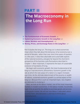
  • 14. 9780199236824_000_000_CH03.qxd 2/2/09 11:06 AM Page 64 64 PART II THE MACROECONOMY IN THE LONG RUN (a) Investment Rate and Real GDP per Capita (level) 60,000 Europe America Level of real GDP per capita in 2004 (in US$) 50,000 Asia Africa 40,000 30,000 20,000 10,000 0 0 5 10 15 20 25 30 35 40 Average investment rate (% of GDP) (b) Investment Rate and Real Growth in GDP per Capita (% per annum) 9.0 Europe Growth in real GDP per capita (% per annum) America Asia Africa 6.0 3.0 0.0 –3.0 0 5 10 15 20 25 30 35 40 Average investment rate (% of GDP) Fig. 3.5 Investment, GDP per Capita, and Real GDP Growth For a sample of 174 countries over the period of 1950–2004, the correlation coefficient between the investment rate (the ratio of investment to GDP) and the average per capita GDP over the period is high and positive (0.51). The correlation of the investment rate in the countries with real GDP growth is also positive but less striking (0.31). Source: Penn World Table Version 6.2 September 2006. © Oxdord University Press 2009. Michael Burda and Charles Wyplosz. Macroeconomics A European Text 5e
  • 15. 9780199236824_000_000_CH03.qxd 2/2/09 11:06 AM Page 65 CHAPTER 3 THE FUNDAMENTALS OF ECONOMIC GROWTH 65 B 3.3.5 The Golden Rule f (k) A Figure 3.6 contains an important message: to become richer, you need to save and invest more. Output–labour ratio Depreciation But is being richer—in the narrow sense of accu- s′f(k) mulating capital goods—always necessarily better? sf(k) Saving requires the sacrifice of giving up some con- sumption today against the promise of higher income tomorrow, but does saving more today always mean more consumption tomorrow? The answer is not necessarily positive. To see why, note O Capital–labour ratio that in the steady state, when the capital stock Fig. 3.6 An Increase in the Savings Rate per capita is Q, savings equal depreciation and the An increase in the savings rate raises capital intensity (k) steady-state level of consumption N (the part of and the output–labour ratio ( y). income that is not saved) is given by: (3.10) N = Y − sY = f (Q) − δQ. In Figure 3.7, consumption per capita is given give the impression that higher investment rates by the vertical distance between the production cause higher economic growth. The boost is only function and the depreciation line.13 If we could temporary: once the steady state has been reached, choose the saving rate, we could e3ectively pick no further growth e3ect can be expected from a any point of intersection of the savings schedule higher savings rate. We still need a story to explain with the depreciation line, and therefore any level growth in output per capita. This is the story told in of consumption we so desired. Figure 3.7 shows Sections 3.4 and 3.5. that consumption is highest at the capital stock for It may be surprising that increased savings does which the slope of the production function is paral- not a3ect long-run growth. The reason that higher lel to the depreciation line.14 The corresponding savings cannot cause capital and output to grow optimal steady-state capital–labour ratio is indic- forever is the assumption of diminishing returns. ated as Q ′. Now remember that the slope of the An increase in savings causes the capital stock to production function is the marginal productivity of rise, but as more capital is put into place, more capital (MPK) while the slope of the depreciation capital depreciates and thus needs to be replaced. schedule is the rate of depreciation δ. We have just Increasing amounts of gross investment are needed shown that the maximal level of consumption is just to keep the capital stock constant at its higher achieved when level. Yet the resources for that increased invest- (3.11) MPK = δ. ment are not forthcoming, because the marginal productivity of capital decreases. Further addi- This condition is called the golden rule, and can be tions to the capital–labour ratio yield smaller and thought of as a recipe for achieving the best use of smaller increases in income, and therefore in sav- existing technological capabilities. In this case, with ings. Depreciation, however, rises with the capital no population growth and no technical progress, stock proportionately. Put simply, the decreasing marginal productivity principle implies that, at some point, saving more is simply not worth it.12 13 Note that everything, including consumption and saving, is measured as a ratio to the labour input, person-hours. As already noted, if the number of hours worked does not change, the ratios move exactly as per capita consumption, 12 In Chapter 4, we will see that the outcome is very di3erent saving, output, etc. when the marginal productivity of capital is not declining. 14 An exercise asks you to prove this assertion. © Oxdord University Press 2009. Michael Burda and Charles Wyplosz. Macroeconomics A European Text 5e
  • 16. 9780199236824_000_000_CH03.qxd 2/2/09 11:06 AM Page 66 66 PART II THE MACROECONOMY IN THE LONG RUN too much capital has been accumulated, and the y = f(k) ′ MPK is lower than the depreciation rate δ. By reduc- A ing savings today, an economy can actually increase Depreciation Y′ per capita consumption, both today and in the future. This looks like a free lunch, and indeed, Output–labour ratio Consumption it is one. We say that the economy su3ers from dynamic inefficiency. Dynamically ine5cient eco- nomies simply save and invest too much and consume too little. Investment A di3erent situation arises if the economy is to the left of Q ′. Here, steady-state income and con- Q′ sumption per capita may be raised by saving more, Capital–labour ratio but not immediately; consumption only can be increased in the long run after the adjustment Fig. 3.7 The Golden Rule has occurred. No free lunch is immediately avail- Steady-state consumption N (as a ratio to labour) is the able, but must be ‘earned’ by increased saving vertical distance between the production function and and reduced consumption at the outset. Moving the depreciation line Q . It is at a maximum at point A towards Q ′ from a position on the left requires cur- corresponding to Q , where the slope of the production rent generations to sacrifice so future generations function, the marginal productivity of capital, is equal can enjoy more consumption which will result to d, the slope of the depreciation line. from more capital and income in the steady state. An economy in such a situation is called dynamically efficient because it is not possible to do better without paying the price for it. The di3erence the golden rule states that the economy maximizes between dynamically e5cient and ine5cient sav- steady-state consumption when the marginal gain ings rates is illustrated in Figure 3.8, which shows from an additional unit of GDP saved and invested how we move from one steady state to another one in capital (MPK) equals the depreciation rate. with higher consumption. What are the consequences of ‘disobeying’ the In the dynamically ine5cient case (a), it is possible golden rule? If the capital–labour ratio exceeds Q ′, to permanently raise consumption by consuming Consumption Consumption Time Time (a) Dynamically inefficient case (b) Dynamically efficient case Fig. 3.8 Raising Steady-State Consumption In a dynamically inefficient economy (a), it is possible to permanently raise consumption by reducing saving. In a dynamically efficient economy (b), higher future consumption requires early sacrifices. © Oxdord University Press 2009. Michael Burda and Charles Wyplosz. Macroeconomics A European Text 5e
  • 17. 9780199236824_000_000_CH03.qxd 2/2/09 11:06 AM Page 67 CHAPTER 3 THE FUNDAMENTALS OF ECONOMIC GROWTH 67 more now and during the transition to the new ously short supply. Box 3.3 presents the case of steady state. In the dynamically e5cient case (b), a Poland. higher steady-state level consumption is not free In dynamically e5cient economies, future genera- and implies a transitory period of sacrifice. tions would benefit from raising saving today, but Dynamic ine5ciency arises when excessive sav- those currently alive would lose. Should govern- ings have led to too high a stock of capital. Sav- ments do something about it? Since it would rep- ing must remain forever high merely to replace resent a transfer of revenues from current to future depreciating capital. Dynamic ine5ciency may generations, there is no simple answer. It is truly a have characterized some of the centrally planned deep political choice with no solution since future economies of Central and Eastern Europe. We say generations don’t vote today. A number of factors ‘may’ because the proof that an economy is ine5- influence savings, such as taxation, health and cient lies in showing that its marginal productiv- retirement systems, cultural norms, and social cus- ity of capital is lower than the depreciation rate, tom. Importantly, too, saving and investment are and neither of these is easily measurable. What influenced by political conditions. Political instabil- we do know is that Communist leaders often ity and especially wars, civil or otherwise, can lead boasted about their economies’ high investment to destruction and theft of capital, and hardly rates, which were in fact considerably higher than encourage thrifty behaviour. As we discuss in in the capitalist West. Yet overall standards of Chapter 4, in many of the world’s poorest coun- living were considerably lower than in market tries, property rights are under constant threat economies, and consumer goods were in notori- or non-existent. Box 3.3 Dynamic Inefficiency in Poland? From the period following the Second World War until the steady-state level of GDP per capita, not its growth rate. early 1990s, Poland was a centrally planned economy. In 1980, Poland invested 21.6% of its GDP. By 1990 this Savings and investment decisions for the Polish eco- rate had fallen to 18.3%. In the period 1990–2004 per nomy were taken by the ruling Communist party. The capita consumption rose in Poland from $2,908 to $7,037, panels of Figure 3.9 compare Poland with Italy, a coun- an increase of 142%, compared with 61% in Italy over the try with one of the highest saving rates in Europe. The first same period. Is this proof of dynamic inefficiency, i.e. graph shows the increase in GDP per capita between that a significant part of savings was used merely to 1980 and 1990 (the GDP measure is adjusted for pur- keep up an excessively large stock of capital? Anecdotal chasing power to take into account different price evidence would suggest so. Stories of wasted resources systems). While Italy’s income grew by 25%, Poland’s were common in centrally planned economies: unin- actually shrank by about 5%. The second graph shows the stalled equipment rusting in backyards, new machinery average proportion of GDP dedicated to saving over the prematurely discarded for lack of spare parts, tools ill- same period. Clearly, Poland saved a lot, but received adapted to factory needs, etc. One important cause of nothing for it in terms of income growth. wastage was a reward system for factory managers. As the third and fourth panels of Figure 3.9 show, the These were often based on spending plans, and not on situation was reversed after 1991, when Poland intro- actual output. An alternative interpretation is that the duced free markets and abandoned central planning. investment was in poor quality equipment, which could From 1991 to 2004, per capita GDP increased by 68%, with not match western technology. No matter how we look a lower investment rate than Italy’s (which grew by 17%). at it, savings were not put to their best use in centrally However, our theory predicts that savings affect the planned Poland. © Oxdord University Press 2009. Michael Burda and Charles Wyplosz. Macroeconomics A European Text 5e
  • 18. 9780199236824_000_000_CH03.qxd 2/2/09 11:06 AM Page 68 68 PART II THE MACROECONOMY IN THE LONG RUN GDP growth Investment/GDP GDP growth Investment/GDP (1990 relative to 1980, %) (average 1980–1990, %) (2004 relative to 1991, %) (average 1991–2004, %) 70.00 30.00 70.00 30.00 60.00 60.00 25.00 25.00 50.00 50.00 20.00 20.00 40.00 40.00 30.00 15.00 15.00 30.00 20.00 10.00 10.00 20.00 10.00 5.00 10.00 5.00 0.00 −10.00 0.00 0.00 0.00 Poland Italy Poland Italy Poland Italy Poland Italy Fig. 3.9 Was Centrally Planned Poland Dynamically Inefficient? Despite a high investment and savings rate, Polish per capita GDP shrank during the period 1980–1990 while Italy’s grew. During the transition period, Poland grew much faster, with a lower investment rate than in Italy. Source: Heston, Summers, and Aten (2006). 3.4 Population Growth and Economic Growth A major shortcoming of the previous section is immigration. Overall, more people are at work but that it does not explain permanent, sustained they work shorter hours, so the balance of e3ects is growth, our first stylized fact. Capital accumula- ambiguous. Because the number of hours worked tion, we saw, can explain high living standards and per person cannot and does not rise without bound, growth during the transition to the steady state we will treat it as constant. Then any change in but the law of diminishing returns ultimately kicks person-hours is due to exogenous changes in the in. Clearly, some crucial ingredients are missing. population and employment, and output per person- One of them is population growth, more precisely, hour changes at the same rate as output per capita. growth in the employed labour force. This section Even though population and employment are shows that sustainable long-run growth of both growing, the fundamental reasoning of Section 3.3 output and the capital stock is possible once we remains valid: the economy gravitates to a steady introduce population growth. state at which the capital–labour and output– Recall that labour input (person-hours) grows labour ratios (k = K/L and y = Y/L) stabilize. With L grow- either if the number of people at work increases, or ing at the exogenous rate n, output Y and capital K if workers work more hours on average. Later on in will also grow at rate n. The relentless increase in this chapter and Chapter 5, we will see that the the labour input is the driver of growth in this case. number of hours worked per person has declined Quite simply, if income per capita is to remain steadily over the past century and a half. Figure 3.10 unchanged in the steady state, income must grow at shows that, despite this fact, employment has been the same rate as the number of people. rising, either because of natural demographic The role of saving and capital accumulation forces (the balance between births and deaths) or remains the same as in the previous section, with only © Oxdord University Press 2009. Michael Burda and Charles Wyplosz. Macroeconomics A European Text 5e