SlideShare une entreprise Scribd logo
1  sur  31
Linear Regression and Correlation
• Explanatory and Response Variables are Numeric
• Relationship between the mean of the response
  variable and the level of the explanatory variable
  assumed to be approximately linear (straight line)
• Model:

   Y = β 0 + β1 x + ε          ε ~ N (0, σ )
  • β1 > 0 ⇒ Positive Association
  • β1 < 0 ⇒ Negative Association
  • β1 = 0 ⇒ No Association
Least Squares Estimation of β0, β1
    ∀ β0 ≡ Mean response when x=0 (y-intercept)
    ∀ β1 ≡ Change in mean response when x increases
      by 1 unit (slope)
    • β0, β1 are unknown parameters (like µ)
    • β0+β1x ≡ Mean response when explanatory
      variable takes on the value x
    • Goal: Choose values (estimates) that minimize the
      sum of squared errors (SSE) of observed values to
      the straight-line:
                                          2                                   2
^    ^   ^
                                     ^
                                            n             ^    ^
                                                                        
                 SSE = ∑i =1  yi − y i  = ∑i =1  yi −  β 0 + β 1 xi  
                            n
y = β 0+ β1 x
                                                                    
Example - Pharmacodynamics of LSD
  • Response (y) - Math score (mean among 5 volunteers)
  • Predictor (x) - LSD tissue concentration (mean of 5 volunteers)
  • Raw Data and scatterplot of Score vs LSD concentration:
                                                      80


                                                      70


                                                      60
    Score (y)                  LSD Conc (x)
     78.93                         1.17               50
     58.20                         2.97
     67.47                         3.26               40

     37.47                         4.69
     45.65                         5.83               30
                                              SCORE


     32.92                         6.00
                                                      20
     29.97                         6.41                    1     2    3   4   5   6   7


                                                           LSD_CONC
Source: Wagner, et al (1968)
Least Squares Computations
S xx =∑−
       x x(    )    2


S xy    =∑ − )(y − )
          (x x    y

         ∑− )
          (y y      2
S yy    =


β=
^
  ∑ − )(y − ) =
   (x x    y   S                xy


   ∑− )
     (x x
    1                       2
               S                xx


β          β
^           ^
 0      = − 1 x
         y

                        2
               
                ^
         ∑ − 
          
           y  y
                 =SSE
s2      =
          n− 2     n−2
Example - Pharmacodynamics of LSD
     Score (y)   LSD Conc (x)   x-xbar    y-ybar      Sxx           Sxy          Syy
      78.93          1.17       -3.163    28.843   10.004569    -91.230409    831.918649
      58.20          2.97       -1.363    8.113     1.857769    -11.058019    65.820769
      67.47          3.26       -1.073    17.383    1.151329    -18.651959    302.168689
      37.47          4.69        0.357   -12.617    0.127449     -4.504269    159.188689
      45.65          5.83        1.497    -4.437    2.241009     -6.642189    19.686969
      32.92          6.00        1.667   -17.167    2.778889    -28.617389    294.705889
      29.97          6.41        2.077   -20.117    4.313929    -41.783009    404.693689
      350.61        30.33       -0.001    0.001    22.474943   -202.487243   2078.183343


(Column totals given in bottom row of table)

    350.61                   30.33
y=         = 50.087       x=       = 4.333
      7                         7
^    − 202.4872               ^        ^
β1 =             = − 9.01    β 0 = y − β 1 x = 50.09 − (− 9.01)(4.33) = 89.10
       22.4749
 ^
y = 89.10 − 9.01x          s 2 = 50.72
SPSS Output and Plot of Equation
                                                   Coefficientsa


                                   Unstandardized               Standardized
                                      Coefficients              Coefficients
Model                               B         Std. Error            Beta                 t                  Sig.
1       (Constant)                 89.124          7.048                                12.646                 .000
        LSD_CONC                   -9.009          1.503                        -.937   -5.994                 .002
  a. Dependent Variable: SCORE


                             Math Score vs LSD Concentration (SPSS)

                    80.00      
                                                                                        Linear Regression


                    70.00
                                               


                    60.00
                                           
            score


                    50.00

                                                                        


                    40.00
                                                            


                                                                            
                                                                                
                    30.00
                                            score = 89.12 + -9.01 * lsd_conc
                            1.00   2.00     R-Square = 0.88 5.00
                                          3.00      4.00                 6.00


                                               lsd_conc
Inference Concerning the Slope (β1)

• Parameter: Slope in the population model (β1)
                                        ^
• Estimator: Least squares estimate: β 1
• Estimated standard error: σ β = s / S
                               ^
                                    ^
                                     1       xx


• Methods of making inference regarding population:
   – Hypothesis tests (2-sided or 1-sided)
   – Confidence Intervals
Hypothesis Test for β1

• 2-Sided Test                      • 1-sided Test
    – H0: β1 = 0                          – H0: β1 = 0
    – HA: β1 ≠ 0                          – HA+: β1 > 0 or
                                          – HA-: β1 < 0
                   ^
                  β1                                ^
T .S . : tobs =   ^              T .S . : tobs =
                                                   β1
                σ β1   ^                           ^
                                                   σ β1
                                                     ^


R.R. : | tobs | ≥ tα / 2,n − 2   R.R.+ : tobs ≥ tα ,n − 2   R.R.− : tobs ≤ − tα ,n − 2
P − val : 2 P(t ≥| tobs |)       P − val + : P (t ≥ tobs ) P − val − : P (t ≤ tobs )
(1-α)100% Confidence Interval for β1

             ^            ^        ^             s
             β 1 ± tα / 2 σ β 1 ≡ β 1 ± tα / 2
                              ^


                                                 S xx

• Conclude positive association if entire interval above 0
• Conclude negative association if entire interval below 0
• Cannot conclude an association if interval contains 0
• Conclusion based on interval is same as 2-sided hypothesis test
Example - Pharmacodynamics of LSD
               ^
   n = 7 β 1 = −9.01 s = 50.72 = 7.12 S xx = 22.475
    ^         7.12
   σ β1 ^
            =        = 1.50
              22.475

    • Testing H0: β1 = 0 vs HA: β1 ≠ 0

                      − 9.01
    T .S . : tobs   =        = −6.01   R.R. :| tobs |≥ t.025,5 = 2.571
                      1.50

    • 95% Confidence Interval for β1 :

− 9.01 ± 2.571(1.50) ≡ − 9.01 ± 3.86 ≡ (−12.87,−5.15)
Correlation Coefficient
• Measures the strength of the linear association
  between two variables
• Takes on the same sign as the slope estimate from
  the linear regression
• Not effected by linear transformations of y or x
• Does not distinguish between dependent and
  independent variable (e.g. height and weight)
• Population Parameter - ρ
• Pearson’s Correlation Coefficient:
                    S xy
             r=                  −1 ≤ r ≤1
                   S xx S yy
Correlation Coefficient
• Values close to 1 in absolute value ⇒ strong
  linear association, positive or negative from sign
• Values close to 0 imply little or no association
• If data contain outliers (are non-normal),
  Spearman’s coefficient of correlation can be
  computed based on the ranks of the x and y values
• Test of H0:ρ = 0 is equivalent to test of H0:β1=0
• Coefficient of Determination (r2) - Proportion of
  variation in y “explained” by the regression on x:
                    S yy − SSE
         r = (r ) =
          2      2
                                 0 ≤ r2 ≤ 1
                         S yy
Example - Pharmacodynamics of LSD
    S xx = 22.475                                       S xy = −202.487            S yy = 2078.183                                           SSE = 253.89
                           − 202.487
   r=                                     = −0.94
                      ( 22.475)(2078.183)
       2078.183 − 253.89
   r =   2
                         = 0.88 = ( −0.94) 2
           2078.183

                                Syy                                                                     SSE
        80.00                                                                      80.00   
                
                                                                    Mean                                                                        Linear Regression


                                                                                   70.00
        70.00                                                                                               
                                  


                                                                                   60.00
        60.00                                                                                           
                            
                                                                           score
score


                                                                                   50.00
        50.00
                                                                                                                                 
                                             Mean = 50.09
                                                     

                                                                                   40.00
        40.00                                                                                                          
                                             
                                                                                                                                     
                                                                                                                                        
                                                                                   30.00
                                                                                                   score = 89.12 + -9.01 * lsd_conc
        30.00
                                                                                       1.00    2.00 R-Square = 0.88
                                                                                                       3.00     4.00     5.00    6.00
             1.00   2.00   3.00       4.00       5.00    6.00
                                                                                                            lsd_conc
                                lsd_conc
Example - SPSS Output
  Pearson’s and Spearman’s Measures
                                    Correlations

                                                         SCORE      LSD_CONC
SCORE                 Pearson Correlation                       1        -.937**
                      Sig. (2-tailed)                           .         .002
                      N                                         7            7
LSD_CONC              Pearson Correlation                   -.937**          1
                      Sig. (2-tailed)                        .002            .
                      N                                         7            7
    **. Correlation is significant at the 0.01 level (2-tailed).


                                       Correlations

                                                                 SCORE     LSD_CONC
Spearman's rho      SCORE            Correlation Coefficient       1.000        -.929**
                                     Sig. (2-tailed)                   .         .003
                                     N                                 7            7
                    LSD_CONC         Correlation Coefficient       -.929**      1.000
                                     Sig. (2-tailed)                .003            .
                                     N                                 7            7
  **. Correlation is significant at the 0.01 level (2-tailed).
Analysis of Variance in Regression
• Goal: Partition the total variation in y into
  variation “explained” by x and random variation
                           ^           ^
   ( yi − y ) = ( yi − y i ) + ( y i − y )
                                           ^       2   ^       2

   ∑ ( y − y) = ∑ ( y − y ) + ∑ ( y − y)
                   2
          i                      i             i           i

 • These three sums of squares and degrees of freedom are:
    •Total (Syy)       dfTotal = n-1

    • Error (SSE)      dfError = n-2

    • Model (SSR)       dfModel = 1
Analysis of Variance in Regression

Source of                  Sum of          Degrees of       Mean
Variation                  Squares          Freedom        Square              F
Model                       SSR                1         MSR = SSR/1      F = MSR/MSE
Error                       SSE               n-2       MSE = SSE/(n-2)
Total                        Syy              n-1


            • Analysis of Variance - F-test
            • H0: β1 = 0             HA: β1 ≠ 0
                                  MSR
            T .S . : Fobs       =
                                 MSE
            R.R. : Fobs         ≥Fα1, n −
                                   ,     2

            P−val : P ( F ≥Fobs )
Example - Pharmacodynamics of LSD

       • Total Sum of squares:

    S yy = ∑ ( yi − y ) 2 = 2078.183    dfTotal = 7 − 1 = 6

        • Error Sum of squares:
                    ^
    SSE = ∑ ( yi − y i ) 2 = 253.890   df Error = 7 − 2 = 5

         • Model Sum of Squares:
           ^
SSR = ∑ ( y i − y ) 2 = 2078.183 − 253.890 = 1824.293         df Model = 1
Example - Pharmacodynamics of LSD
Source of            Sum of          Degrees of    Mean
Variation            Squares          Freedom      Square      F
Model               1824.293             1        1824.293   35.93
Error               253.890              5         50.778
Total               2078.183             6


     •Analysis of Variance - F-test
     • H0: β1 = 0              HA: β1 ≠ 0
                        MSR
   T .S . : Fobs      =          = .93
                                  35
                       MSE
   R.R. : Fobs        ≥F.05,1, 5 = .61
                                  6
   P−val : P ( F ≥ .93)
                  35
Example - SPSS Output

                                        ANOVAb

                       Sum of
Model                 Squares           df       Mean Square    F       Sig.
1       Regression    1824.302               1      1824.302   35.928      .002a
        Residual       253.881               5        50.776
        Total         2078.183               6
  a. Predictors: (Constant), LSD_CONC
  b. Dependent Variable: SCORE
Multiple Regression

• Numeric Response variable (Y)
• p Numeric predictor variables
• Model:
   Y = β0 + β1x1 + ⋅⋅⋅ + βpxp + ε


• Partial Regression Coefficients: βi ≡ effect (on the
  mean response) of increasing the ith predictor
  variable by 1 unit, holding all other predictors
  constant
Example - Effect of Birth weight on
         Body Size in Early Adolescence
   • Response: Height at Early adolescence (n =250 cases)
   • Predictors (p=6 explanatory variables)
       • Adolescent Age (x1, in years -- 11-14)
       • Tanner stage (x2, units not given)
       • Gender (x3=1 if male, 0 if female)
       • Gestational age (x4, in weeks at birth)
       • Birth length (x5, units not given)
                • Birthweight Group (x6=1,...,6 <1500g (1), 1500-
                1999g(2), 2000-2499g(3), 2500-2999g(4), 3000-
                3499g(5), >3500g(6))
Source: Falkner, et al (2004)
Least Squares Estimation

     • Population Model for mean response:

         E (Y ) = β 0 + β1 x1 +  + β p x p

    • Least Squares Fitted (predicted) equation, minimizing SSE:

                                                                     2
^    ^     ^               ^
                                                               ^
Y = β 0 + β 1 x1 +  + β p x p           SSE = ∑  Y − Y 
                                                        
     • All statistical software packages/spreadsheets can
     compute least squares estimates and their standard errors
Analysis of Variance
     • Direct extension to ANOVA based on simple
       linear regression
     • Only adjustments are to degrees of freedom:
            – dfModel = p         dfError = n-p-1

Source of               Sum of             Degrees of        Mean
Variation               Squares             Freedom         Square               F
Model                    SSR                   p          MSR = SSR/p       F = MSR/MSE
Error                    SSE                 n-p-1      MSE = SSE/(n-p-1)
Total                     Syy                 n-1


                                        S yy − SSE        SSR
                             R =  2
                                                        =
                                             S yy         S yy
Testing for the Overall Model - F-test
• Tests whether any of the explanatory variables are
  associated with the response
• H0: β1=⋅⋅⋅=βp=0 (None of the xs associated with y)
• HA: Not all βi = 0
                   MSR               R2 / p
 T .S . : Fobs   =          =
                  MSE          (1 − 2 ) /( n −p − )
                                   R             1
 R.R. : Fobs     ≥Fα p , n −p −
                    ,          1

 P−val : P ( F ≥Fobs )
Example - Effect of Birth weight on
        Body Size in Early Adolescence
 • Authors did not print ANOVA, but did provide following:
     • n=250      p=6   R2=0.26
 • H0: β1=⋅⋅⋅=β6=0
 • HA: Not all βi = 0


                MSR            R2 / p
T .S . : Fobs =        =                     =
                MSE      (1 −R ) /( n −p − )
                              2
                                          1
              0.26 / 6          .0433
=                             =        = .2
                                         14
   (1 − .26) /( 250 − − )
         0              6 1     .0030
R.R. : Fobs ≥Fα 6 , 243 =2.13
                   ,

P−val : P ( F ≥ .2)
               14
Testing Individual Partial Coefficients - t-tests
  • Wish to determine whether the response is
    associated with a single explanatory variable, after
    controlling for the others


  • H0: βi = 0             HA: βi ≠ 0 (2-sided alternative)
                           ^
                          βi
      T .S . : t obs =    ^
                         σβ    ^
                                   i


      R.R. : | t obs | ≥ tα / 2 , n − p −1
      P − val : 2 P (t ≥| tobs |)
Example - Effect of Birth weight on
   Body Size in Early Adolescence
Variable               b      sb    t=b/sb P-val (z)
Adolescent Age       2.86    0.99    2.89     .0038
Tanner Stage         3.41    0.89    3.83     <.001
Male                 0.08    1.26    0.06     .9522
Gestational Age      -0.11 0.21     -0.52     .6030
Birth Length         0.44    0.19    2.32     .0204
Birth Wt Grp         -0.78 0.64     -1.22     .2224

Controlling for all other predictors, adolescent age,
Tanner stage, and Birth length are associated with
adolescent height measurement
Models with Dummy Variables
• Some models have both numeric and categorical
  explanatory variables (Recall gender in example)
• If a categorical variable has k levels, need to create
  k-1 dummy variables that take on the values 1 if
  the level of interest is present, 0 otherwise.
• The baseline level of the categorical variable for
  which all k-1 dummy variables are set to 0
• The regression coefficient corresponding to a
  dummy variable is the difference between the
  mean for that level and the mean for baseline
  group, controlling for all numeric predictors
Example - Deep Cervical Infections
     • Subjects - Patients with deep neck infections
     • Response (Y) - Length of Stay in hospital
     • Predictors: (One numeric, 11 Dichotomous)
              – Age (x1)
              – Gender (x2=1 if female, 0 if male)
              – Fever (x3=1 if Body Temp > 38C, 0 if not)
              – Neck swelling (x4=1 if Present, 0 if absent)
              – Neck Pain (x5=1 if Present, 0 if absent)
              – Trismus (x6=1 if Present, 0 if absent)
              – Underlying Disease (x7=1 if Present, 0 if absent)
              – Respiration Difficulty (x8=1 if Present, 0 if absent)
              – Complication (x9=1 if Present, 0 if absent)
              – WBC > 15000/mm3 (x10=1 if Present, 0 if absent)
              – CRP > 100µg/ml (x11=1 if Present, 0 if absent)
Source: Wang, et al (2003)
Example - Weather and Spinal Patients
                   • Subjects - Visitors to National Spinal Network in 23 cities
                     Completing SF-36 Form
                   • Response - Physical Function subscale (1 of 10 reported)
                   • Predictors:
                               – Patient’s age (x1)
                               – Gender (x2=1 if female, 0 if male)
                               – High temperature on day of visit (x3)
                               – Low temperature on day of visit (x4)
                               – Dew point (x5)
                               – Wet bulb (x6)
                               – Total precipitation (x7)
                               – Barometric Pressure (x7)
                               – Length of sunlight (x8)
                               – Moon Phase (new, wax crescent, 1st Qtr, wax gibbous, full moon,
Source: Glaser, et al (2004)
                                 wan gibbous, last Qtr, wan crescent, presumably had 8-1=7
Analysis of Covariance
• Combination of 1-Way ANOVA and Linear
  Regression
• Goal: Comparing numeric responses among k
  groups, adjusting for numeric concomitant
  variable(s), referred to as Covariate(s)
• Clinical trial applications: Response is Post-Trt
  score, covariate is Pre-Trt score
• Epidemiological applications: Outcomes
  compared across exposure conditions, adjusted for
  other risk factors (age, smoking status, sex,...)

Contenu connexe

Tendances

Mesh Processing Course : Multiresolution
Mesh Processing Course : MultiresolutionMesh Processing Course : Multiresolution
Mesh Processing Course : MultiresolutionGabriel Peyré
 
Low Complexity Regularization of Inverse Problems
Low Complexity Regularization of Inverse ProblemsLow Complexity Regularization of Inverse Problems
Low Complexity Regularization of Inverse ProblemsGabriel Peyré
 
5icdsa2007 v4
5icdsa2007 v45icdsa2007 v4
5icdsa2007 v4fminhos
 
Signal Processing Course : Convex Optimization
Signal Processing Course : Convex OptimizationSignal Processing Course : Convex Optimization
Signal Processing Course : Convex OptimizationGabriel Peyré
 
Introduction to Gaussian Processes
Introduction to Gaussian ProcessesIntroduction to Gaussian Processes
Introduction to Gaussian ProcessesDmytro Fishman
 
Low Complexity Regularization of Inverse Problems - Course #1 Inverse Problems
Low Complexity Regularization of Inverse Problems - Course #1 Inverse ProblemsLow Complexity Regularization of Inverse Problems - Course #1 Inverse Problems
Low Complexity Regularization of Inverse Problems - Course #1 Inverse ProblemsGabriel Peyré
 
Low Complexity Regularization of Inverse Problems - Course #3 Proximal Splitt...
Low Complexity Regularization of Inverse Problems - Course #3 Proximal Splitt...Low Complexity Regularization of Inverse Problems - Course #3 Proximal Splitt...
Low Complexity Regularization of Inverse Problems - Course #3 Proximal Splitt...Gabriel Peyré
 
Signal Processing Course : Inverse Problems Regularization
Signal Processing Course : Inverse Problems RegularizationSignal Processing Course : Inverse Problems Regularization
Signal Processing Course : Inverse Problems RegularizationGabriel Peyré
 
Proximal Splitting and Optimal Transport
Proximal Splitting and Optimal TransportProximal Splitting and Optimal Transport
Proximal Splitting and Optimal TransportGabriel Peyré
 
On Convergence of Jungck Type Iteration for Certain Contractive Conditions
On Convergence of Jungck Type Iteration for Certain Contractive ConditionsOn Convergence of Jungck Type Iteration for Certain Contractive Conditions
On Convergence of Jungck Type Iteration for Certain Contractive Conditionsresearchinventy
 
Regression Theory
Regression TheoryRegression Theory
Regression TheorySSA KPI
 
Mesh Processing Course : Active Contours
Mesh Processing Course : Active ContoursMesh Processing Course : Active Contours
Mesh Processing Course : Active ContoursGabriel Peyré
 
Prediction of Financial Processes
Prediction of Financial ProcessesPrediction of Financial Processes
Prediction of Financial ProcessesSSA KPI
 
Probability and Statistics Cookbook
Probability and Statistics CookbookProbability and Statistics Cookbook
Probability and Statistics CookbookChairat Nuchnuanrat
 

Tendances (20)

Mesh Processing Course : Multiresolution
Mesh Processing Course : MultiresolutionMesh Processing Course : Multiresolution
Mesh Processing Course : Multiresolution
 
Low Complexity Regularization of Inverse Problems
Low Complexity Regularization of Inverse ProblemsLow Complexity Regularization of Inverse Problems
Low Complexity Regularization of Inverse Problems
 
5icdsa2007 v4
5icdsa2007 v45icdsa2007 v4
5icdsa2007 v4
 
Signal Processing Course : Convex Optimization
Signal Processing Course : Convex OptimizationSignal Processing Course : Convex Optimization
Signal Processing Course : Convex Optimization
 
Introduction to Gaussian Processes
Introduction to Gaussian ProcessesIntroduction to Gaussian Processes
Introduction to Gaussian Processes
 
Low Complexity Regularization of Inverse Problems - Course #1 Inverse Problems
Low Complexity Regularization of Inverse Problems - Course #1 Inverse ProblemsLow Complexity Regularization of Inverse Problems - Course #1 Inverse Problems
Low Complexity Regularization of Inverse Problems - Course #1 Inverse Problems
 
Low Complexity Regularization of Inverse Problems - Course #3 Proximal Splitt...
Low Complexity Regularization of Inverse Problems - Course #3 Proximal Splitt...Low Complexity Regularization of Inverse Problems - Course #3 Proximal Splitt...
Low Complexity Regularization of Inverse Problems - Course #3 Proximal Splitt...
 
BS1501 tutorial 2
BS1501 tutorial 2BS1501 tutorial 2
BS1501 tutorial 2
 
Signal Processing Course : Inverse Problems Regularization
Signal Processing Course : Inverse Problems RegularizationSignal Processing Course : Inverse Problems Regularization
Signal Processing Course : Inverse Problems Regularization
 
Proximal Splitting and Optimal Transport
Proximal Splitting and Optimal TransportProximal Splitting and Optimal Transport
Proximal Splitting and Optimal Transport
 
03 finding roots
03 finding roots03 finding roots
03 finding roots
 
On Convergence of Jungck Type Iteration for Certain Contractive Conditions
On Convergence of Jungck Type Iteration for Certain Contractive ConditionsOn Convergence of Jungck Type Iteration for Certain Contractive Conditions
On Convergence of Jungck Type Iteration for Certain Contractive Conditions
 
Geometry Transformation
Geometry TransformationGeometry Transformation
Geometry Transformation
 
Presentation
PresentationPresentation
Presentation
 
Ch05 6
Ch05 6Ch05 6
Ch05 6
 
Meja kursi
Meja kursiMeja kursi
Meja kursi
 
Regression Theory
Regression TheoryRegression Theory
Regression Theory
 
Mesh Processing Course : Active Contours
Mesh Processing Course : Active ContoursMesh Processing Course : Active Contours
Mesh Processing Course : Active Contours
 
Prediction of Financial Processes
Prediction of Financial ProcessesPrediction of Financial Processes
Prediction of Financial Processes
 
Probability and Statistics Cookbook
Probability and Statistics CookbookProbability and Statistics Cookbook
Probability and Statistics Cookbook
 

Similaire à Linreg (20)

Jacobi and gauss-seidel
Jacobi and gauss-seidelJacobi and gauss-seidel
Jacobi and gauss-seidel
 
BS2506 tutorial3
BS2506 tutorial3BS2506 tutorial3
BS2506 tutorial3
 
Presentation on Regression Analysis
Presentation on Regression AnalysisPresentation on Regression Analysis
Presentation on Regression Analysis
 
talk9.ppt
talk9.ppttalk9.ppt
talk9.ppt
 
Correlation & regression
Correlation & regression Correlation & regression
Correlation & regression
 
Regresi Ni3.Nf
Regresi Ni3.NfRegresi Ni3.Nf
Regresi Ni3.Nf
 
Regression.Doc Rini
Regression.Doc RiniRegression.Doc Rini
Regression.Doc Rini
 
Regression.Doc Rini
Regression.Doc RiniRegression.Doc Rini
Regression.Doc Rini
 
Regression.Doc Rini
Regression.Doc RiniRegression.Doc Rini
Regression.Doc Rini
 
Sparsenet
SparsenetSparsenet
Sparsenet
 
Correlation & regression uwsb
Correlation & regression   uwsbCorrelation & regression   uwsb
Correlation & regression uwsb
 
Measures of variation and dispersion report
Measures of variation and dispersion reportMeasures of variation and dispersion report
Measures of variation and dispersion report
 
Root locus
Root locusRoot locus
Root locus
 
Unit 3
Unit 3Unit 3
Unit 3
 
Numerical Methods Solving Linear Equations
Numerical Methods Solving Linear EquationsNumerical Methods Solving Linear Equations
Numerical Methods Solving Linear Equations
 
regression
regressionregression
regression
 
Regression
RegressionRegression
Regression
 
PART I.3 - Physical Mathematics
PART I.3 - Physical MathematicsPART I.3 - Physical Mathematics
PART I.3 - Physical Mathematics
 
Multiple Regression Case
Multiple Regression CaseMultiple Regression Case
Multiple Regression Case
 
Pydata Katya Vasilaky
Pydata Katya VasilakyPydata Katya Vasilaky
Pydata Katya Vasilaky
 

Dernier

Tampa BSides - Chef's Tour of Microsoft Security Adoption Framework (SAF)
Tampa BSides - Chef's Tour of Microsoft Security Adoption Framework (SAF)Tampa BSides - Chef's Tour of Microsoft Security Adoption Framework (SAF)
Tampa BSides - Chef's Tour of Microsoft Security Adoption Framework (SAF)Mark Simos
 
DevoxxFR 2024 Reproducible Builds with Apache Maven
DevoxxFR 2024 Reproducible Builds with Apache MavenDevoxxFR 2024 Reproducible Builds with Apache Maven
DevoxxFR 2024 Reproducible Builds with Apache MavenHervé Boutemy
 
Streamlining Python Development: A Guide to a Modern Project Setup
Streamlining Python Development: A Guide to a Modern Project SetupStreamlining Python Development: A Guide to a Modern Project Setup
Streamlining Python Development: A Guide to a Modern Project SetupFlorian Wilhelm
 
The Ultimate Guide to Choosing WordPress Pros and Cons
The Ultimate Guide to Choosing WordPress Pros and ConsThe Ultimate Guide to Choosing WordPress Pros and Cons
The Ultimate Guide to Choosing WordPress Pros and ConsPixlogix Infotech
 
Commit 2024 - Secret Management made easy
Commit 2024 - Secret Management made easyCommit 2024 - Secret Management made easy
Commit 2024 - Secret Management made easyAlfredo García Lavilla
 
From Family Reminiscence to Scholarly Archive .
From Family Reminiscence to Scholarly Archive .From Family Reminiscence to Scholarly Archive .
From Family Reminiscence to Scholarly Archive .Alan Dix
 
Developer Data Modeling Mistakes: From Postgres to NoSQL
Developer Data Modeling Mistakes: From Postgres to NoSQLDeveloper Data Modeling Mistakes: From Postgres to NoSQL
Developer Data Modeling Mistakes: From Postgres to NoSQLScyllaDB
 
Ensuring Technical Readiness For Copilot in Microsoft 365
Ensuring Technical Readiness For Copilot in Microsoft 365Ensuring Technical Readiness For Copilot in Microsoft 365
Ensuring Technical Readiness For Copilot in Microsoft 3652toLead Limited
 
SIP trunking in Janus @ Kamailio World 2024
SIP trunking in Janus @ Kamailio World 2024SIP trunking in Janus @ Kamailio World 2024
SIP trunking in Janus @ Kamailio World 2024Lorenzo Miniero
 
What's New in Teams Calling, Meetings and Devices March 2024
What's New in Teams Calling, Meetings and Devices March 2024What's New in Teams Calling, Meetings and Devices March 2024
What's New in Teams Calling, Meetings and Devices March 2024Stephanie Beckett
 
DSPy a system for AI to Write Prompts and Do Fine Tuning
DSPy a system for AI to Write Prompts and Do Fine TuningDSPy a system for AI to Write Prompts and Do Fine Tuning
DSPy a system for AI to Write Prompts and Do Fine TuningLars Bell
 
H2O.ai CEO/Founder: Sri Ambati Keynote at Wells Fargo Day
H2O.ai CEO/Founder: Sri Ambati Keynote at Wells Fargo DayH2O.ai CEO/Founder: Sri Ambati Keynote at Wells Fargo Day
H2O.ai CEO/Founder: Sri Ambati Keynote at Wells Fargo DaySri Ambati
 
"ML in Production",Oleksandr Bagan
"ML in Production",Oleksandr Bagan"ML in Production",Oleksandr Bagan
"ML in Production",Oleksandr BaganFwdays
 
Dev Dives: Streamline document processing with UiPath Studio Web
Dev Dives: Streamline document processing with UiPath Studio WebDev Dives: Streamline document processing with UiPath Studio Web
Dev Dives: Streamline document processing with UiPath Studio WebUiPathCommunity
 
Merck Moving Beyond Passwords: FIDO Paris Seminar.pptx
Merck Moving Beyond Passwords: FIDO Paris Seminar.pptxMerck Moving Beyond Passwords: FIDO Paris Seminar.pptx
Merck Moving Beyond Passwords: FIDO Paris Seminar.pptxLoriGlavin3
 
Artificial intelligence in cctv survelliance.pptx
Artificial intelligence in cctv survelliance.pptxArtificial intelligence in cctv survelliance.pptx
Artificial intelligence in cctv survelliance.pptxhariprasad279825
 
How AI, OpenAI, and ChatGPT impact business and software.
How AI, OpenAI, and ChatGPT impact business and software.How AI, OpenAI, and ChatGPT impact business and software.
How AI, OpenAI, and ChatGPT impact business and software.Curtis Poe
 
Anypoint Exchange: It’s Not Just a Repo!
Anypoint Exchange: It’s Not Just a Repo!Anypoint Exchange: It’s Not Just a Repo!
Anypoint Exchange: It’s Not Just a Repo!Manik S Magar
 
TrustArc Webinar - How to Build Consumer Trust Through Data Privacy
TrustArc Webinar - How to Build Consumer Trust Through Data PrivacyTrustArc Webinar - How to Build Consumer Trust Through Data Privacy
TrustArc Webinar - How to Build Consumer Trust Through Data PrivacyTrustArc
 

Dernier (20)

DMCC Future of Trade Web3 - Special Edition
DMCC Future of Trade Web3 - Special EditionDMCC Future of Trade Web3 - Special Edition
DMCC Future of Trade Web3 - Special Edition
 
Tampa BSides - Chef's Tour of Microsoft Security Adoption Framework (SAF)
Tampa BSides - Chef's Tour of Microsoft Security Adoption Framework (SAF)Tampa BSides - Chef's Tour of Microsoft Security Adoption Framework (SAF)
Tampa BSides - Chef's Tour of Microsoft Security Adoption Framework (SAF)
 
DevoxxFR 2024 Reproducible Builds with Apache Maven
DevoxxFR 2024 Reproducible Builds with Apache MavenDevoxxFR 2024 Reproducible Builds with Apache Maven
DevoxxFR 2024 Reproducible Builds with Apache Maven
 
Streamlining Python Development: A Guide to a Modern Project Setup
Streamlining Python Development: A Guide to a Modern Project SetupStreamlining Python Development: A Guide to a Modern Project Setup
Streamlining Python Development: A Guide to a Modern Project Setup
 
The Ultimate Guide to Choosing WordPress Pros and Cons
The Ultimate Guide to Choosing WordPress Pros and ConsThe Ultimate Guide to Choosing WordPress Pros and Cons
The Ultimate Guide to Choosing WordPress Pros and Cons
 
Commit 2024 - Secret Management made easy
Commit 2024 - Secret Management made easyCommit 2024 - Secret Management made easy
Commit 2024 - Secret Management made easy
 
From Family Reminiscence to Scholarly Archive .
From Family Reminiscence to Scholarly Archive .From Family Reminiscence to Scholarly Archive .
From Family Reminiscence to Scholarly Archive .
 
Developer Data Modeling Mistakes: From Postgres to NoSQL
Developer Data Modeling Mistakes: From Postgres to NoSQLDeveloper Data Modeling Mistakes: From Postgres to NoSQL
Developer Data Modeling Mistakes: From Postgres to NoSQL
 
Ensuring Technical Readiness For Copilot in Microsoft 365
Ensuring Technical Readiness For Copilot in Microsoft 365Ensuring Technical Readiness For Copilot in Microsoft 365
Ensuring Technical Readiness For Copilot in Microsoft 365
 
SIP trunking in Janus @ Kamailio World 2024
SIP trunking in Janus @ Kamailio World 2024SIP trunking in Janus @ Kamailio World 2024
SIP trunking in Janus @ Kamailio World 2024
 
What's New in Teams Calling, Meetings and Devices March 2024
What's New in Teams Calling, Meetings and Devices March 2024What's New in Teams Calling, Meetings and Devices March 2024
What's New in Teams Calling, Meetings and Devices March 2024
 
DSPy a system for AI to Write Prompts and Do Fine Tuning
DSPy a system for AI to Write Prompts and Do Fine TuningDSPy a system for AI to Write Prompts and Do Fine Tuning
DSPy a system for AI to Write Prompts and Do Fine Tuning
 
H2O.ai CEO/Founder: Sri Ambati Keynote at Wells Fargo Day
H2O.ai CEO/Founder: Sri Ambati Keynote at Wells Fargo DayH2O.ai CEO/Founder: Sri Ambati Keynote at Wells Fargo Day
H2O.ai CEO/Founder: Sri Ambati Keynote at Wells Fargo Day
 
"ML in Production",Oleksandr Bagan
"ML in Production",Oleksandr Bagan"ML in Production",Oleksandr Bagan
"ML in Production",Oleksandr Bagan
 
Dev Dives: Streamline document processing with UiPath Studio Web
Dev Dives: Streamline document processing with UiPath Studio WebDev Dives: Streamline document processing with UiPath Studio Web
Dev Dives: Streamline document processing with UiPath Studio Web
 
Merck Moving Beyond Passwords: FIDO Paris Seminar.pptx
Merck Moving Beyond Passwords: FIDO Paris Seminar.pptxMerck Moving Beyond Passwords: FIDO Paris Seminar.pptx
Merck Moving Beyond Passwords: FIDO Paris Seminar.pptx
 
Artificial intelligence in cctv survelliance.pptx
Artificial intelligence in cctv survelliance.pptxArtificial intelligence in cctv survelliance.pptx
Artificial intelligence in cctv survelliance.pptx
 
How AI, OpenAI, and ChatGPT impact business and software.
How AI, OpenAI, and ChatGPT impact business and software.How AI, OpenAI, and ChatGPT impact business and software.
How AI, OpenAI, and ChatGPT impact business and software.
 
Anypoint Exchange: It’s Not Just a Repo!
Anypoint Exchange: It’s Not Just a Repo!Anypoint Exchange: It’s Not Just a Repo!
Anypoint Exchange: It’s Not Just a Repo!
 
TrustArc Webinar - How to Build Consumer Trust Through Data Privacy
TrustArc Webinar - How to Build Consumer Trust Through Data PrivacyTrustArc Webinar - How to Build Consumer Trust Through Data Privacy
TrustArc Webinar - How to Build Consumer Trust Through Data Privacy
 

Linreg

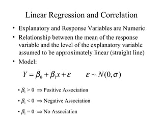
  • 1. Linear Regression and Correlation • Explanatory and Response Variables are Numeric • Relationship between the mean of the response variable and the level of the explanatory variable assumed to be approximately linear (straight line) • Model: Y = β 0 + β1 x + ε ε ~ N (0, σ ) • β1 > 0 ⇒ Positive Association • β1 < 0 ⇒ Negative Association • β1 = 0 ⇒ No Association
  • 2. Least Squares Estimation of β0, β1 ∀ β0 ≡ Mean response when x=0 (y-intercept) ∀ β1 ≡ Change in mean response when x increases by 1 unit (slope) • β0, β1 are unknown parameters (like µ) • β0+β1x ≡ Mean response when explanatory variable takes on the value x • Goal: Choose values (estimates) that minimize the sum of squared errors (SSE) of observed values to the straight-line: 2 2 ^ ^ ^  ^  n   ^ ^  SSE = ∑i =1  yi − y i  = ∑i =1  yi −  β 0 + β 1 xi   n y = β 0+ β1 x     
  • 3. Example - Pharmacodynamics of LSD • Response (y) - Math score (mean among 5 volunteers) • Predictor (x) - LSD tissue concentration (mean of 5 volunteers) • Raw Data and scatterplot of Score vs LSD concentration: 80 70 60 Score (y) LSD Conc (x) 78.93 1.17 50 58.20 2.97 67.47 3.26 40 37.47 4.69 45.65 5.83 30 SCORE 32.92 6.00 20 29.97 6.41 1 2 3 4 5 6 7 LSD_CONC Source: Wagner, et al (1968)
  • 4. Least Squares Computations S xx =∑− x x( ) 2 S xy =∑ − )(y − ) (x x y ∑− ) (y y 2 S yy = β= ^ ∑ − )(y − ) = (x x y S xy ∑− ) (x x 1 2 S xx β β ^ ^ 0 = − 1 x y 2   ^ ∑ −   y y  =SSE s2 = n− 2 n−2
  • 5. Example - Pharmacodynamics of LSD Score (y) LSD Conc (x) x-xbar y-ybar Sxx Sxy Syy 78.93 1.17 -3.163 28.843 10.004569 -91.230409 831.918649 58.20 2.97 -1.363 8.113 1.857769 -11.058019 65.820769 67.47 3.26 -1.073 17.383 1.151329 -18.651959 302.168689 37.47 4.69 0.357 -12.617 0.127449 -4.504269 159.188689 45.65 5.83 1.497 -4.437 2.241009 -6.642189 19.686969 32.92 6.00 1.667 -17.167 2.778889 -28.617389 294.705889 29.97 6.41 2.077 -20.117 4.313929 -41.783009 404.693689 350.61 30.33 -0.001 0.001 22.474943 -202.487243 2078.183343 (Column totals given in bottom row of table) 350.61 30.33 y= = 50.087 x= = 4.333 7 7 ^ − 202.4872 ^ ^ β1 = = − 9.01 β 0 = y − β 1 x = 50.09 − (− 9.01)(4.33) = 89.10 22.4749 ^ y = 89.10 − 9.01x s 2 = 50.72
  • 6. SPSS Output and Plot of Equation Coefficientsa Unstandardized Standardized Coefficients Coefficients Model B Std. Error Beta t Sig. 1 (Constant) 89.124 7.048 12.646 .000 LSD_CONC -9.009 1.503 -.937 -5.994 .002 a. Dependent Variable: SCORE Math Score vs LSD Concentration (SPSS) 80.00  Linear Regression 70.00  60.00  score 50.00  40.00    30.00 score = 89.12 + -9.01 * lsd_conc 1.00 2.00 R-Square = 0.88 5.00 3.00 4.00 6.00 lsd_conc
  • 7. Inference Concerning the Slope (β1) • Parameter: Slope in the population model (β1) ^ • Estimator: Least squares estimate: β 1 • Estimated standard error: σ β = s / S ^ ^ 1 xx • Methods of making inference regarding population: – Hypothesis tests (2-sided or 1-sided) – Confidence Intervals
  • 8. Hypothesis Test for β1 • 2-Sided Test • 1-sided Test – H0: β1 = 0 – H0: β1 = 0 – HA: β1 ≠ 0 – HA+: β1 > 0 or – HA-: β1 < 0 ^ β1 ^ T .S . : tobs = ^ T .S . : tobs = β1 σ β1 ^ ^ σ β1 ^ R.R. : | tobs | ≥ tα / 2,n − 2 R.R.+ : tobs ≥ tα ,n − 2 R.R.− : tobs ≤ − tα ,n − 2 P − val : 2 P(t ≥| tobs |) P − val + : P (t ≥ tobs ) P − val − : P (t ≤ tobs )
  • 9. (1-α)100% Confidence Interval for β1 ^ ^ ^ s β 1 ± tα / 2 σ β 1 ≡ β 1 ± tα / 2 ^ S xx • Conclude positive association if entire interval above 0 • Conclude negative association if entire interval below 0 • Cannot conclude an association if interval contains 0 • Conclusion based on interval is same as 2-sided hypothesis test
  • 10. Example - Pharmacodynamics of LSD ^ n = 7 β 1 = −9.01 s = 50.72 = 7.12 S xx = 22.475 ^ 7.12 σ β1 ^ = = 1.50 22.475 • Testing H0: β1 = 0 vs HA: β1 ≠ 0 − 9.01 T .S . : tobs = = −6.01 R.R. :| tobs |≥ t.025,5 = 2.571 1.50 • 95% Confidence Interval for β1 : − 9.01 ± 2.571(1.50) ≡ − 9.01 ± 3.86 ≡ (−12.87,−5.15)
  • 11. Correlation Coefficient • Measures the strength of the linear association between two variables • Takes on the same sign as the slope estimate from the linear regression • Not effected by linear transformations of y or x • Does not distinguish between dependent and independent variable (e.g. height and weight) • Population Parameter - ρ • Pearson’s Correlation Coefficient: S xy r= −1 ≤ r ≤1 S xx S yy
  • 12. Correlation Coefficient • Values close to 1 in absolute value ⇒ strong linear association, positive or negative from sign • Values close to 0 imply little or no association • If data contain outliers (are non-normal), Spearman’s coefficient of correlation can be computed based on the ranks of the x and y values • Test of H0:ρ = 0 is equivalent to test of H0:β1=0 • Coefficient of Determination (r2) - Proportion of variation in y “explained” by the regression on x: S yy − SSE r = (r ) = 2 2 0 ≤ r2 ≤ 1 S yy
  • 13. Example - Pharmacodynamics of LSD S xx = 22.475 S xy = −202.487 S yy = 2078.183 SSE = 253.89 − 202.487 r= = −0.94 ( 22.475)(2078.183) 2078.183 − 253.89 r = 2 = 0.88 = ( −0.94) 2 2078.183 Syy SSE 80.00 80.00   Mean Linear Regression 70.00 70.00   60.00 60.00   score score 50.00 50.00  Mean = 50.09  40.00 40.00      30.00  score = 89.12 + -9.01 * lsd_conc 30.00 1.00 2.00 R-Square = 0.88 3.00 4.00 5.00 6.00 1.00 2.00 3.00 4.00 5.00 6.00 lsd_conc lsd_conc
  • 14. Example - SPSS Output Pearson’s and Spearman’s Measures Correlations SCORE LSD_CONC SCORE Pearson Correlation 1 -.937** Sig. (2-tailed) . .002 N 7 7 LSD_CONC Pearson Correlation -.937** 1 Sig. (2-tailed) .002 . N 7 7 **. Correlation is significant at the 0.01 level (2-tailed). Correlations SCORE LSD_CONC Spearman's rho SCORE Correlation Coefficient 1.000 -.929** Sig. (2-tailed) . .003 N 7 7 LSD_CONC Correlation Coefficient -.929** 1.000 Sig. (2-tailed) .003 . N 7 7 **. Correlation is significant at the 0.01 level (2-tailed).
  • 15. Analysis of Variance in Regression • Goal: Partition the total variation in y into variation “explained” by x and random variation ^ ^ ( yi − y ) = ( yi − y i ) + ( y i − y ) ^ 2 ^ 2 ∑ ( y − y) = ∑ ( y − y ) + ∑ ( y − y) 2 i i i i • These three sums of squares and degrees of freedom are: •Total (Syy) dfTotal = n-1 • Error (SSE) dfError = n-2 • Model (SSR) dfModel = 1
  • 16. Analysis of Variance in Regression Source of Sum of Degrees of Mean Variation Squares Freedom Square F Model SSR 1 MSR = SSR/1 F = MSR/MSE Error SSE n-2 MSE = SSE/(n-2) Total Syy n-1 • Analysis of Variance - F-test • H0: β1 = 0 HA: β1 ≠ 0 MSR T .S . : Fobs = MSE R.R. : Fobs ≥Fα1, n − , 2 P−val : P ( F ≥Fobs )
  • 17. Example - Pharmacodynamics of LSD • Total Sum of squares: S yy = ∑ ( yi − y ) 2 = 2078.183 dfTotal = 7 − 1 = 6 • Error Sum of squares: ^ SSE = ∑ ( yi − y i ) 2 = 253.890 df Error = 7 − 2 = 5 • Model Sum of Squares: ^ SSR = ∑ ( y i − y ) 2 = 2078.183 − 253.890 = 1824.293 df Model = 1
  • 18. Example - Pharmacodynamics of LSD Source of Sum of Degrees of Mean Variation Squares Freedom Square F Model 1824.293 1 1824.293 35.93 Error 253.890 5 50.778 Total 2078.183 6 •Analysis of Variance - F-test • H0: β1 = 0 HA: β1 ≠ 0 MSR T .S . : Fobs = = .93 35 MSE R.R. : Fobs ≥F.05,1, 5 = .61 6 P−val : P ( F ≥ .93) 35
  • 19. Example - SPSS Output ANOVAb Sum of Model Squares df Mean Square F Sig. 1 Regression 1824.302 1 1824.302 35.928 .002a Residual 253.881 5 50.776 Total 2078.183 6 a. Predictors: (Constant), LSD_CONC b. Dependent Variable: SCORE
  • 20. Multiple Regression • Numeric Response variable (Y) • p Numeric predictor variables • Model: Y = β0 + β1x1 + ⋅⋅⋅ + βpxp + ε • Partial Regression Coefficients: βi ≡ effect (on the mean response) of increasing the ith predictor variable by 1 unit, holding all other predictors constant
  • 21. Example - Effect of Birth weight on Body Size in Early Adolescence • Response: Height at Early adolescence (n =250 cases) • Predictors (p=6 explanatory variables) • Adolescent Age (x1, in years -- 11-14) • Tanner stage (x2, units not given) • Gender (x3=1 if male, 0 if female) • Gestational age (x4, in weeks at birth) • Birth length (x5, units not given) • Birthweight Group (x6=1,...,6 <1500g (1), 1500- 1999g(2), 2000-2499g(3), 2500-2999g(4), 3000- 3499g(5), >3500g(6)) Source: Falkner, et al (2004)
  • 22. Least Squares Estimation • Population Model for mean response: E (Y ) = β 0 + β1 x1 +  + β p x p • Least Squares Fitted (predicted) equation, minimizing SSE: 2 ^ ^ ^ ^   ^ Y = β 0 + β 1 x1 +  + β p x p SSE = ∑  Y − Y    • All statistical software packages/spreadsheets can compute least squares estimates and their standard errors
  • 23. Analysis of Variance • Direct extension to ANOVA based on simple linear regression • Only adjustments are to degrees of freedom: – dfModel = p dfError = n-p-1 Source of Sum of Degrees of Mean Variation Squares Freedom Square F Model SSR p MSR = SSR/p F = MSR/MSE Error SSE n-p-1 MSE = SSE/(n-p-1) Total Syy n-1 S yy − SSE SSR R = 2 = S yy S yy
  • 24. Testing for the Overall Model - F-test • Tests whether any of the explanatory variables are associated with the response • H0: β1=⋅⋅⋅=βp=0 (None of the xs associated with y) • HA: Not all βi = 0 MSR R2 / p T .S . : Fobs = = MSE (1 − 2 ) /( n −p − ) R 1 R.R. : Fobs ≥Fα p , n −p − , 1 P−val : P ( F ≥Fobs )
  • 25. Example - Effect of Birth weight on Body Size in Early Adolescence • Authors did not print ANOVA, but did provide following: • n=250 p=6 R2=0.26 • H0: β1=⋅⋅⋅=β6=0 • HA: Not all βi = 0 MSR R2 / p T .S . : Fobs = = = MSE (1 −R ) /( n −p − ) 2 1 0.26 / 6 .0433 = = = .2 14 (1 − .26) /( 250 − − ) 0 6 1 .0030 R.R. : Fobs ≥Fα 6 , 243 =2.13 , P−val : P ( F ≥ .2) 14
  • 26. Testing Individual Partial Coefficients - t-tests • Wish to determine whether the response is associated with a single explanatory variable, after controlling for the others • H0: βi = 0 HA: βi ≠ 0 (2-sided alternative) ^ βi T .S . : t obs = ^ σβ ^ i R.R. : | t obs | ≥ tα / 2 , n − p −1 P − val : 2 P (t ≥| tobs |)
  • 27. Example - Effect of Birth weight on Body Size in Early Adolescence Variable b sb t=b/sb P-val (z) Adolescent Age 2.86 0.99 2.89 .0038 Tanner Stage 3.41 0.89 3.83 <.001 Male 0.08 1.26 0.06 .9522 Gestational Age -0.11 0.21 -0.52 .6030 Birth Length 0.44 0.19 2.32 .0204 Birth Wt Grp -0.78 0.64 -1.22 .2224 Controlling for all other predictors, adolescent age, Tanner stage, and Birth length are associated with adolescent height measurement
  • 28. Models with Dummy Variables • Some models have both numeric and categorical explanatory variables (Recall gender in example) • If a categorical variable has k levels, need to create k-1 dummy variables that take on the values 1 if the level of interest is present, 0 otherwise. • The baseline level of the categorical variable for which all k-1 dummy variables are set to 0 • The regression coefficient corresponding to a dummy variable is the difference between the mean for that level and the mean for baseline group, controlling for all numeric predictors
  • 29. Example - Deep Cervical Infections • Subjects - Patients with deep neck infections • Response (Y) - Length of Stay in hospital • Predictors: (One numeric, 11 Dichotomous) – Age (x1) – Gender (x2=1 if female, 0 if male) – Fever (x3=1 if Body Temp > 38C, 0 if not) – Neck swelling (x4=1 if Present, 0 if absent) – Neck Pain (x5=1 if Present, 0 if absent) – Trismus (x6=1 if Present, 0 if absent) – Underlying Disease (x7=1 if Present, 0 if absent) – Respiration Difficulty (x8=1 if Present, 0 if absent) – Complication (x9=1 if Present, 0 if absent) – WBC > 15000/mm3 (x10=1 if Present, 0 if absent) – CRP > 100µg/ml (x11=1 if Present, 0 if absent) Source: Wang, et al (2003)
  • 30. Example - Weather and Spinal Patients • Subjects - Visitors to National Spinal Network in 23 cities Completing SF-36 Form • Response - Physical Function subscale (1 of 10 reported) • Predictors: – Patient’s age (x1) – Gender (x2=1 if female, 0 if male) – High temperature on day of visit (x3) – Low temperature on day of visit (x4) – Dew point (x5) – Wet bulb (x6) – Total precipitation (x7) – Barometric Pressure (x7) – Length of sunlight (x8) – Moon Phase (new, wax crescent, 1st Qtr, wax gibbous, full moon, Source: Glaser, et al (2004) wan gibbous, last Qtr, wan crescent, presumably had 8-1=7
  • 31. Analysis of Covariance • Combination of 1-Way ANOVA and Linear Regression • Goal: Comparing numeric responses among k groups, adjusting for numeric concomitant variable(s), referred to as Covariate(s) • Clinical trial applications: Response is Post-Trt score, covariate is Pre-Trt score • Epidemiological applications: Outcomes compared across exposure conditions, adjusted for other risk factors (age, smoking status, sex,...)