linearization

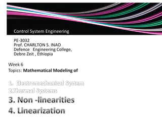
1. Control System Engineering
PE-3032
Prof. CHARLTON S. INAO
Defence Engineering College,
Debre Zeit , Ethiopia

2. Modeling
of
Nonlinearities/
Linearization

3. Nonlinearities
A linear system possesses two properties:
superposition and homogeneity.
• The property of superposition means that the output response of
a system to the sum of inputs is the sum of the responses to the
individual inputs.
Thus, if an input of r1(t) yields an output of c1(t) and
an input of r2(t) yields an output of c2(t), then an input of r1(t) +
r2(t) yields an output of c1(t) + c2(t).
• The property of homogeneity describes the response of the
system to a multiplication of the input by a scalar.
Specifically, in a linear system, the property of
homogeneity is demonstrated if for an input of r1(t) that yields an
output of c1(t), an input of Ar1(t) yields an output of Ac1(t); that
is, multiplication of an input by a scalar yields a response that is
multiplied by the same scalar.

4. We can visualize linearity as shown in Figure 6. Figure 6(a) is a
linear system where the output is always ½ of the input, or f(x) = 0.5X:,
regardless of the value of X, Thus each of the two properties of linear
systems applies.
For example, an input of 1 yields an output of ½ and an input of 2 yields an
output of 1. Using superposition, an input that is the sum of the original
inputs, or 3, should yield an output that is the sum of the individual outputs,
or 1.5. From Figure 6(a), an input of 3 does indeed yield an output of 1.5.
FIGURE 6 a. Linear system; b. nonlinear system
To test the property of
homogeneity, assume an
input of 2, which yields an
output of 1. Multiplying this
input by 2 should yield an
output of twice as much, or 2.
From Figure 6(a), an input of
4 does indeed yield an output
of 2. The reader can verify
that the properties of linearity
certainly do not apply to the
relationship shown in Figure
6(b).

5. Figure 7 shows some examples of physical nonlinearities.
An electronic amplifier is linear over a specific range but
exhibits the nonlinearity called saturation at high input
voltages.
A motor that does not respond at very low input voltages
due to frictional forces exhibits a nonlinearity called dead
zone.
Gears that do not fit tightly exhibit a nonlinearity called
backlash: The input moves over a small range without the
output responding.
The reader should verify that the curves shown in Figure 7
do not fit the definitions of linearity over their entire range.

6. FIGURE 7 Some physical nonlinearities
increasing
decreasing

7. Non Linear Effects (from Aircraft Engine Controls)

8. A designer can often make a linear approximation to a
nonlinear system. Linear approximations simplify the analysis
and design of a system and are used as long as the results
yield a good approximation to reality.
For example, a linear relationship can be established at
a point on the nonlinear curve if the range of input values
about that point is small and the origin is translated to that
point.
 Electronic amplifiers are an example of physical
devices that perform linear amplification with small excursions
about a point.

9. Linearization
The electrical and mechanical systems covered
thus far were assumed to be linear. However,
if any nonlinear components are present, we
must linearize the system before we can find
the transfer function. After discussing and
defining nonlinearities non-linearities, we
show how to obtain linear approximations to
nonlinear systems in order to obtain transfer
functions or to model a physical system.

10. The first step is to recognize the nonlinear component and
write the nonlinear differential equation. When we linearize a
nonlinear differential equation, we linearize it for small-signal inputs
about the steady-state solution when the small-signal input is equal
to zero. This steady-state solution is called equilibrium and is
selected as the second step in the linearization process. For
example, when a pendulum is at rest, it is at equilibrium. The
angular displacement is described by a nonlinear differential
equation, but it can be expressed with a linear differential equation
for small excursions about this equilibrium point.
Next we linearize the nonlinear differential equation, and then
we take the Laplace transform of the linearized differential equation,
assuming zero initial conditions. Finally, we separate input and output
variables and form the transfer function. Let us first see how to
linearize a function; later, we will apply the method to the linearization
of a differential equation.

11. Linearization Rules

12. If we assume a nonlinear system operating at point A, [x0, f(x0)] in Figure
8, small changes in the input can be related to changes in the output about
the point by way of the slope of the curve at the point A. Thus, if the slope
of the curve at point A is ma, then small excursions of the input about point
A, δx, yield small changes in the output, δf(x), related by the slope at point
A. Thus,
FIGURE 8 Linearization about points
Eq. 3.0
Eq. 3.1
Eq. 3.2
This relationship is shown graphically in
Figure 8, where a new set of axes, δx
and δf(x), is created at the point A, and
f(x) is approximately equal to f(x0), the
ordinate of the new origin, plus small
excursions, maδx, away from point A.

13. Linearization of NonLinear Systems
by Taylor Series/Expansion

15. Example: Linearizing a Function
Sample 1: Linearize f(x) = 5cosx about x=π/2.
SOLUTION:
• We first find that the derivative of f(x) is df/dx=(-
5sinx). At x=π/2, the derivative is -5. Also f(x0) =
f(π /2) = 5cos(π/2) = 0. Thus, from Eq. (3.2), the
system can be represented as f(x) = -5δx for small
excursions of x about π/2. The process is shown
graphically in Figure 9, where the cosine curve
does indeed look like a straight line of slope -5
near π/2.

16. FIGURE 9 Linearization of 5cos x about x = π/2

17. The previous discussion can be formalized using the Taylor series
expansion, which expresses the value of a function in terms of the value of that
function at a particular point, the excursion away from that point, and derivatives
evaluated at that point. The Taylor series is shown in Eq. (3.3).
For small excursions of x from xo, we can neglect higher-order
terms. The resulting approximation yields a straight-line relationship between the
change in f(x) and the excursions away from XQ. Neglecting the higher-order
terms in Eq. (3.3), we get
Eq.3.3
Eq. 3.4
or
Eq. 35.
which is a linear relationship between δf(x)
and δx for small excursions away from x0.
It is interesting to note that Eqs. (3.4) and
(3.5) are identical to Eqs. (3.0) and (3.1),
which we derived intuitively.

18. Linearization Sample Problem 2

19. Linearization Sample Problem 2
cont……..
a b

20. Linearization Sample Problem 3
Derivative of nonlinear

21. Graph of z=x2
+4xy+6y2
z=x^2+4xy+6y^2
Non linear
z x y
131 1 -5
68 2 -4
27 3 -3
8 4 -2
11 5 -1
36 6 0
83 7 1
152 8 2
243 9 3
356 10 4
491 11 5
648 12 6
827 13 7
1028 14 8
1251 15 9
1496 16 10
1763 17 11
2052 18 12
2363 19 13
2696 20 14
3051 21 15
3428 22 16
3827 23 17
X=9, y=3

22. z=30x+72y+243
z x y
-63 6 0
39 7 1
141 8 2
243 9 3
345 10 4
447 11 5
549 12 6
651 13 7
753 14 8
855 15 9
957 16 10
1059 17 11
1161 18 12
1263 19 13
1365 20 14
1467 21 15
1569 22 16
1671 23 17
1773 24 18
1875 25 19
1977 26 20
2079 27 21
2181 28 22
2283 29 23

23. Linearization Sample Problem 4

24. Derivative of nonlinear

25. Graph of z=x2
+8xy+3y2

27. Y against z
Y=11, z=636

28. Graph of z with x value shown(non linear)
3
636 3 11
731 3.5 11.5
832 4 12
939 4.5 12.5
1052 5 13
1171 5.5 13.5
1296 6 14
1427 6.5 14.5
1564 7 15
1707 7.5 15.5
1856 8 16
2011 8.5 16.5
2172 9 17
2339 9.5 17.5
2512 10 18
2691 10.5 18.5
2876 11 19
3067 11.5 19.5
3264 12 20
3467 12.5 20.5
3676 13 21
z x y

29. linear
z x y
268 1 9
360 1.5 9.5
452 2 10
544 2.5 10.5
636 3 11
728 3.5 11.5
820 4 12
912 4.5 12.5
1004 5 13
1096 5.5 13.5
1188 6 14
1280 6.5 14.5
1372 7 15
1464 7.5 15.5
1556 8 16
1648 8.5 16.5
1740 9 17
1832 9.5 17.5
1924 10 18
2016 10.5 18.5
2108 11 19
2200 11.5 19.5
2292 12 20
2384 12.5 20.5
2476 13 21

31. Linearization Sample Problem 5
Derivative of nonlinear
differential equation
Substituting x=2
Linearized equation