SlideShare a Scribd company logo
1 of 13
Download to read offline
1
Application of Bernoulli’s Equation: Flow
measurement
Measuring devices:
The pitot tube and the pitot-static tube
The venturi meter
Orifices
Bernoulli’s Equation
𝑝 + 𝑑𝑝 𝐴 + 𝑑𝐴
𝑝𝐴
𝑑𝑠
𝜃
𝜌𝑔𝐴 𝑑𝑠
Force momentum relation applied to steady, 1D, inviscid fluid flow
𝑑𝑧
Consider a small stream tube having length ds
For an inviscid flow, shear stresses are absent
𝐹𝑠𝑦𝑠 = 𝜌𝑄 𝑉2 − 𝑉1
− 𝑝 + 𝑑𝑝 𝐴 + 𝑑𝐴 + 𝑝𝐴 − 𝜌𝑔𝐴 𝑑𝑠 𝑆𝑖𝑛𝜃 = 𝜌𝑄 𝑉2 − 𝑉1
−𝑑𝑝 𝐴 − 𝜌𝑔𝐴 𝑑𝑧 = 𝜌𝑄 𝑑𝑉
−𝑑𝑝 𝐴 − 𝜌𝑔𝐴 𝑑𝑧 = 𝜌𝐴 𝑉 𝑑𝑉
𝑑𝑝 + 𝜌𝑔 𝑑𝑧 + 𝜌 𝑉 𝑑𝑉 = 0Euler’s equation
For a constant density fluid 𝑑 𝑝 + 𝜌𝑔𝑧 + 𝜌𝑉2
/2 = 0 𝑑 𝑝/𝜌𝑔 + 𝑧 + 𝑉2
/2𝑔 = 0
𝑝 + 𝜌𝑔𝑧 + 𝜌𝑉2
/2 = 𝐶𝑜𝑛𝑠𝑡𝑎𝑛𝑡
𝑝/𝜌𝑔 + 𝑧 + 𝑉2
/2𝑔 = 𝐶𝑜𝑛𝑠𝑡𝑎𝑛𝑡
Total pressure is constant along a streamline
Total head is constant along a streamline
or
1D Frictionless flow in a converging pipe
𝜃
Datum z=0
Total head
Piezometric head line
𝑃1
𝜌𝑔
𝑉1
2
2𝑔
𝑍1
𝑍2
𝑃2
𝜌𝑔
𝑉2
2
2𝑔
𝐴1
𝐴2
𝑃
𝜌𝑔
+ 𝑧 +
𝑉2
2𝑔
= 𝐻
Consider a stream of uniform velocity flows into a blunt body
Stream line pattern
Apply Bernoulli equation to central streamline (1)
and (2)
𝑃1
𝜌𝑔
+
𝑉1
2
2𝑔
+ 𝑍1 =
𝑃2
𝜌𝑔
+
𝑉2
2
2𝑔
+ 𝑍2
𝑉2 = 0; 𝑍1 = 𝑍2
𝑃1
𝜌𝑔
+
𝑉1
2
2𝑔
=
𝑃2
𝜌𝑔
𝑃2 = 𝑃1 +
1
2
𝜌𝑉1
2
Stagnation
Pressure
Static
Pressure
Dynamic
Pressure
Pitot tube
2
A piezometer and a pitot tube
Two piezometers, one as normal and one as a Pitot tube within the pipe can be used in
an arrangement shown below to measure velocity of flow
𝑃2 = 𝑃1 +
1
2
𝜌𝑉1
2
𝜌𝑔ℎ2 = 𝜌𝑔ℎ1 +
1
2
𝜌𝑉1
2
𝑉1 = 2𝑔 ℎ2 − ℎ1
Pitot tube
1
2
Pitot tube
Pitot-static tube
Close-up of a Pitot-static tube
Pitot-static tube
A pitot tube is connected to a manometer. The holes on the side of the tube connect to one side of a
manometer and register the static head, (h1), while the central hole is connected to the other side of the
manometer to register, as before, the stagnation head (h2).
1
2
𝜌𝑉1
2
= 𝜌𝑔ℎ − 𝜌 𝑚𝑎𝑛 𝑔ℎ
𝑉1 =
2𝑔ℎ
𝜌
𝜌 − 𝜌 𝑚
The Pitot/Pitot-static tubes give velocities at points in the
flow
Pitot-static tube
(1)
(1)
(2)
A B
h
x
Connected point (1)
Connected point (2)
Consider the pressures on the level of the centre line
of the Pitot tube
𝑃1 + 𝜌𝑔𝑥 = 𝑃2 + 𝜌𝑔(𝑥 − ℎ) + 𝜌 𝑚𝑎𝑛 𝑔ℎ
𝑃2 = 𝑃1 + 𝜌𝑔ℎ − 𝜌 𝑚𝑎𝑛 𝑔ℎ
𝑃2 = 𝑃1 +
1
2
𝜌𝑉1
2
Applying Bernoulli equation
3
Bernoulli equation:
𝑃1
𝜌𝑔
+
𝑉1
2
2𝑔
+ 𝑍1 =
𝑃2
𝜌𝑔
+
𝑉2
2
2𝑔
+ 𝑍2
Carefully designed to minimize the energy losses
Converging section: 𝒅𝒑
𝒅𝒙 < 𝟎
Favorable pressure gradient, Stable flow, negligible
energy loss
Diverging section: 𝒅𝒑
𝒅𝒙 > 0
Adverse pressure gradient: Unstable flow, energy loss
Converging section
(1)
(2)
Δh
h2=P2/ρg
h1=P1/ρg
𝑃1
𝜌𝑔
+ 𝑧1 −
𝑃2
𝜌𝑔
+ 𝑧2 =
𝑉2
2
2𝑔
−
𝑉1
2
2𝑔
∆ℎ =
𝑄2
2𝑔
1
𝐴2
2 −
1
𝐴1
2
𝑄 = 𝐴1 𝐴2
2𝑔∆ℎ
𝐴1
2
− 𝐴2
2
Continuity equation:
𝑄 = 𝐴1 𝑉1 = 𝐴2 𝑉2; 𝐴2 < 𝐴1; 𝑉2 > 𝑉1
; 𝑉1 = 𝐴2
2𝑔∆ℎ
𝐴1
2 − 𝐴2
2
Constriction flow meters
Orifice meter
Flow nozzle
Venturi meter
Constriction flow meters
In terms of the manometer readings
𝑃1 + 𝜌𝑔𝑍1 = 𝑃2 + 𝜌𝑔(𝑍2 − ℎ) + 𝜌 𝑚𝑎𝑛 𝑔ℎ
𝑃1 − 𝑃2
𝜌𝑔
+ 𝑍1 − 𝑍2 = ℎ
𝜌 𝑚𝑎𝑛
𝜌
− 1
𝑉1 = 𝐴2
2𝑔
𝑃1 − 𝑃2
𝜌𝑔 + 𝑍1 − 𝑍2
𝐴1
2 − 𝐴2
2
𝑉1 = 𝐴2
2𝑔ℎ
𝜌 𝑚𝑎𝑛
𝜌
− 1
𝐴1
2
− 𝐴2
2
𝑄 𝑎𝑐𝑡 = 𝐶 𝑑 𝐴1 𝐴2
2𝑔ℎ
𝜌 𝑚𝑎𝑛
𝜌
− 1
𝐴1
2 − 𝐴2
2
Venturi meter
About 200
About 60
Z2
Z1 h
Datum
Streamline pattern
Orifice meter
RoundedSharp-edge Square shoulder
Thick-plate square
edge
Orifice in a pipe
4
‘small orifice’: orifice diameter is small compared to head producing flow (head does not vary across the
orifice)
h
P0 (1)
(2)
0 open
to atm
0 Tank is
large 0
Torricelli’s theorem: Velocity of a issuing jet is proportional to the square root of the head producing
flow
Liquid
flow
Small orifice
Applying Bernoulli’s equation to (1) and 2)
𝑃1
𝜌𝑔
+ 𝑍1 +
𝑉1
2
2𝑔
=
𝑃2
𝜌𝑔
+ 𝑍2 +
𝑉2
2
2𝑔
𝑉2 = 2𝑔ℎ ; 𝑄 = 𝑎 2𝑔ℎ
Vena Contractor
Actual area
Vena Contractor
Actual area
In practice, actual discharge is less than the theoretical discharge
Reasons:
Actual velocity <Theoretical velocity due to energy loss between (1) and (2)
𝑉𝑎𝑐𝑡 = 𝐶 𝑣 2𝑔ℎ 𝐶𝑣− coefficient of velocity
Fluid path converges on the orifice. Area is less than the orifice area
𝐴 𝑎𝑐𝑡 = 𝐶𝑐 𝐴 𝑜𝑟𝑖𝑓𝑖𝑐𝑒; 𝐶𝑐- coefficient of contraction
𝑄 𝑎𝑐𝑡 = 𝐶𝑣 2𝑔ℎ . 𝐶𝑐 𝐴 𝑜𝑟𝑖𝑓𝑖𝑐𝑒
Coefficient of discharge 𝐶 𝑑 = 𝐶𝑐 𝐶 𝑣
Coefficient of discharge depends on the edge condition
𝐶𝑐 ≈ 1
𝐶𝑣 ≈ 0.98
𝐶 𝑑 ≈ 0.98
𝐶𝑐 ≈ 1
𝐶𝑣 ≈ 0.86
𝐶 𝑑 ≈ 0.86
𝐶𝑐 ≈ 0.62
𝐶𝑣 ≈ 0.98
𝐶 𝑑 ≈ 0.61
𝐶𝑐 ≈ 0.62
𝐶𝑣 ≈ 0.98
𝐶 𝑑 ≈ 0.61
*Contraction of jet
RoundedSharp-edge Square shoulder Thick-plate square edge
Determination of the coefficient of contraction, velocity, and discharge (Cc , Cv , and Cd)
x
y
H
𝑢 𝑡ℎ𝑒𝑜𝑟𝑒𝑡𝑖𝑐𝑎𝑙 = 2𝑔𝐻
𝑈𝐴 = 𝐶𝑣 𝑉𝑇
𝐶𝑣 =
𝑔
2𝑦 𝑥
2𝑔𝐻
𝐶𝑣 =
𝑥2
4𝑦𝐻
𝐶 𝑑 =
𝑄 𝐴
𝑄 𝑇
𝑄 𝑇 = a 2𝑔ℎ
𝑄 𝐴 √ Use direct method
𝐶𝑐 =
𝐶 𝑑
𝐶𝑣
𝑥 = 𝑢𝑡; 𝑡 = 𝑥
𝑢
𝑦 =
1
2
𝑔𝑡2
𝑢 =
𝑔
2𝑦
𝑥
5
Falling head method: Determine coefficient of discharge (For any outflow
device)
𝑄 = 𝐴𝑉
𝑄 = 𝐴
𝑑ℎ
𝑑𝑡
A
𝑑ℎ
𝑑𝑡
= 𝑄𝑖𝑛 − 𝑄 𝑜𝑢𝑡
𝑄𝑖𝑛=0; 𝑄 𝑜𝑢𝑡 = 𝐶 𝑑 𝑎 2𝑔𝐻 for small orifice
A
𝑑ℎ
𝑑𝑡
= −𝐶 𝑑 𝑎 2𝑔𝐻
𝑑𝑡 = −
𝐴
𝐶 𝑑 𝑎 2𝑔 𝑑
𝑑ℎ
ℎ0.5
𝑡 = −
2𝐴
𝐶 𝑑 𝑎 2𝑔 𝑑
ℎ0.5
+ 𝐶
𝑡 = 0;ℎ = ℎ1
𝑡 = 𝑇; ℎ = ℎ2
𝑇 =
2𝐴
𝐶 𝑑 𝑎 2𝑔
ℎ1
0.5
− ℎ2
0.5
h1
h2
Area A
Orifice area =a
Exercise
A large tank contains a liquid to a depth z. A small orifice located at height y above the tank base
discharges a horizontal jet to the atmosphere. The jet strikes the base level of the tank at a
horizontal distance x. Assume 𝐶𝑣 = 1 , 𝐶𝑐 = 0.63, 𝐴 = 670𝑎
(i) Show that 𝑥2
+ 4𝑦2
= 4𝑦𝑧 and that the maximum horizontal distance occurs when 𝑧 = 2𝑦
(ii) Given y=0.25 m, find the time taken for the jet striking distance x to change from 𝑥1 = 1𝑚 to
𝑥2 = 0.5𝑚
h1
h2
x
y
z
Exercise: Approach velocity (𝑽 𝟎) correction
H=2.5 m
P0 (0)
(1)
Liquid
flow
Area: A
Area: a
𝑃0
𝜌𝑔
+ 𝑍0 +
𝑉0
2
2𝑔
=
𝑃1
𝜌𝑔
+ 𝑍1 +
𝑉1
2
2𝑔
𝑍0 +
𝑉0
2
2𝑔
=𝑍1 +
𝑉1
2
2𝑔
𝑉0
2
2𝑔
+ 𝐻=
𝑉1
2
2𝑔
𝐴0 𝑉0 = 𝐴1 𝑉1
Applying continuity equation:
𝑉0 =
𝑎
𝐴
𝑉1
𝑎
𝐴
2 𝑉1
2
2𝑔
+ 𝐻=
𝑉1
2
2𝑔
𝑉 =
2𝑔𝐻
1 −
𝑎2
𝐴2
A/a V
5 ?
10 ?
100 ?
1000 ?
𝑉 = 2𝑔𝐻 = 7 𝑚/𝑠
Assumed small area; if orifice area is not small
h1
h2
𝑉1 = 2𝑔ℎ1
𝑉2 = 2𝑔ℎ2
Velocity will change across the orifice
Head vary substantially from top to bottom
6
For small area dA;
𝑉 = 2𝑔ℎ
𝑑𝑄 = 𝑏𝑑ℎ 2𝑔ℎ
Large rectangular orifice: vertical height is large
h1
h2
h
dh
*Side contraction
Integrate over area;
𝑄 = 𝑏 2𝑔 ℎ. 𝑑ℎ
ℎ2
ℎ1
𝑄 = 𝐶 𝑑
2𝑏
3
2𝑔 ℎ2
3/2
− ℎ1
3/2
Notches and weirs
Notch: Opening in the side of a tank or reservoir, extending above the free surface (No
upper edge)
Weir: notch on a large scale, to measure the flow of a river
Rectangular notch
b
H
h
𝑄 = 𝐶 𝑑
2𝑏
3
2𝑔 𝐻3/2
𝑄 = 𝐶 𝑑
2𝑏
3
2𝑔 ℎ2
3/2
− ℎ1
3/2
0
𝑑𝐴 = 2 𝐻 − ℎ 𝑇𝑎𝑛𝜃. 𝑑ℎ
𝑑𝑄 = 2𝑔ℎ .2 𝐻 − ℎ 𝑇𝑎𝑛𝜃. 𝑑ℎ
𝑑𝑄 = 2 2𝑔 𝑡𝑎𝑛𝜃. ℎ1/2
𝐻 − ℎ
𝐻
0
𝑑ℎ
𝑄 𝑎𝑐𝑡 = 𝐶 𝑑
8
15
2𝑔 𝑡𝑎𝑛𝜃 𝐻5/2
Vee notch
H
h
Weir Calibration
For a V notch:
Applying mass continuity equation (assume quasi steady condition)
𝐴
𝑑𝐻
𝑑𝑡
= 𝑄𝑖𝑛 − 𝑄 𝑜𝑢𝑡 = 0 − 𝐶 𝑑
8
15
2𝑔 𝑡𝑎𝑛𝜃 𝐻
5
2
Integrating:
𝑇 =
5𝐴
4𝐶 𝑑
𝐻2
−3/2
− 𝐻1
−3/2
𝑡𝑎𝑛𝜃 2𝑔
7
Angular momentum equation
Moment of momentum equation
For a particle dm having velocity 𝑉 ;
Linear momentum = 𝑉.dm
Moment about axis on O = 𝑟 x 𝑉.dm
𝐻0 = 𝑟 x 𝑉.dm
𝑠𝑦𝑠
H- moment of momentum
𝑉𝑡 𝑇𝑟𝑒𝑛𝑠𝑣𝑒𝑟𝑠𝑒 𝑡𝑎𝑛𝑔𝑒𝑛𝑡𝑖𝑎𝑙 𝑣𝑒𝑙𝑜𝑐𝑖𝑡𝑦
𝑉𝑟 𝑅𝑎𝑑𝑖𝑎𝑙 𝑣𝑒𝑙𝑜𝑐𝑖𝑡𝑦
Moment of momentum
Angular momentum equation
Newton’s 2nd law to rotating systems:
𝐹 =
𝑑
𝑑𝑡
𝑚𝑉
𝑟x 𝐹 = 𝑟
𝑑
𝑑𝑡
𝑚𝑉
𝑟x 𝐹 = 𝑑
𝑑𝑡
𝑟 × 𝑚 𝑉
𝑇 =
𝑑𝐻
𝑑𝑡
T net torque or moment applied on the system
Rate of change of moment of momentum (angular momentum) of a system is equal to the net torque acting
on the system
Angular momentum equation-CV Expression
𝐻0 = 𝑟 x 𝑉.dm
𝑠𝑦𝑠
𝑇 =
𝑑𝐻
𝑑𝑡
Newton’s 2nd law to rotating systems
𝑑𝐵𝑠𝑦𝑠
𝑑𝑡
=
𝜕
𝜕𝑡
𝛽𝜌𝑑∀
𝐶𝑉
+ 𝛽
𝐶𝑆
𝜌𝑉. 𝑑𝐴
For a stationary CV, RTT
𝑑𝐵 = 𝛽. 𝑑𝑚 = 𝛽. 𝜌. 𝑑∀
𝐵 = 𝛽. 𝜌. 𝑑∀
𝐶𝑉
Extensive property B = moment of momentum
𝐵 = 𝑟 x 𝑉.dm = 𝑟 x 𝑉.ρ𝑑∀𝐶𝑉𝐶𝑉
𝛽 =
𝑑𝐵
𝑑𝑚
=
𝑑𝐻0
𝑑𝑚
= 𝑟 x 𝑉
CV expression for angular momentum equation
𝑑𝐻 𝑠𝑦𝑠
𝑑𝑡
=
𝜕
𝜕𝑡
𝑟x 𝑉𝜌𝑑∀𝐶𝑉
+ 𝑟 × 𝑉𝐶𝑆
𝜌𝑉. 𝑑𝐴
𝑇 =
𝑑𝐻
𝑑𝑡 𝐶𝑉
+ 𝐻 𝑜
𝑜𝑢𝑡
-𝐻 𝑜
𝑖𝑛
Angular momentum equation-CV Expression Cont.
Steady flow
𝑑𝐻
𝑑𝑡 𝐶𝑉
=0 ;
𝑇 = 𝐻 𝑜
𝑜𝑢𝑡
−𝐻 𝑜
𝑖𝑛
= (𝑟 × 𝑉𝑚) 𝑜𝑢𝑡- (𝑟 × 𝑉𝑚)𝑖𝑛
Steady 1D flow:
𝑇 = ρ𝑄 𝑟2 𝑉2 − 𝑟1 𝑉1
The sum of all external moments
acting on a CV
The rate of change of the angular
momentum of the contents of the
CV
The net rate of angular
momentum out of the control
surface
= +
𝑇 =
𝑑𝐻
𝑑𝑡 𝐶𝑉
+ 𝐻 𝑜
𝑜𝑢𝑡
-𝐻 𝑜
𝑖𝑛
8
Application
Pump
𝑇 = ρ𝑄 𝑟2 𝑉2 − 𝑟1 𝑉1
Fluid EnergyMechanical Energy
Centrifugal Pump
Flow direction
Vt2
Vt1
r2
r1
ω
Example 1
20 cm 30 cm
A Bω
A sprinkler with two nozzles of diameter 4 mm each is connected across a tap of water. The nozzles are at a
distance of 30 cm and 20 cm from the centre of the tap. The flow rate of water through tap is 120 cm3/s. The
nozzles discharge water in the downward direction. Determine the angular speed at which the sprinkler will
rotate free.
2- arm rotating
sprinkler
𝜃
Datum z=0
Total head
Piezometric head line
𝑃1
𝜌𝑔
𝑉1
2
2𝑔
𝑍1
𝑍2
𝑃2
𝜌𝑔
𝑉2
2
2𝑔
𝐴1
𝐴2
𝑃
𝜌𝑔
+ 𝑧 +
𝑉2
2𝑔
= 𝐻
𝑃1
𝜌𝑔
+ 𝑍1 +
𝑉1
2
2𝑔
=
𝑃2
𝜌𝑔
+ 𝑍2 +
𝑉2
2
2𝑔
Consider a streamline between two points 1 and 2
Bernoulli equation Modifications of Bernoulli Equation
In practice, the total energy of a streamline does not remain constant
Consider a streamline between two points 1 and 2
𝐻1 + 𝐻𝑒𝑎𝑑 𝑎𝑑𝑑𝑖𝑡𝑖𝑜𝑛𝑠 − 𝐻𝑒𝑎𝑑 𝑙𝑜𝑠𝑠𝑒𝑠 = 𝐻2 Head balance equation
𝐻1 ∓ 𝐻 𝐸 − 𝐻𝑓 = 𝐻2
𝑃1
𝜌𝑔
+
𝑉1
2
2𝑔
+ 𝑍1 ∓ 𝐻 𝐸 − 𝐻𝑓 =
𝑃2
𝜌𝑔
+
𝑉2
2
2𝑔
+ 𝑍2
(3.12)
Energy is ‘lost’ through friction (actually transformed into heat), and external energy may be either
added by means of a pump or extracted by a turbine
𝜃𝐴1
𝐴2
Losses (transformed into another state)
Additions
9
ℎ 𝑓 = 𝜆
𝐿
𝐷
𝑉2
2𝑔
L (m)
to
to (N/m2)
to
to
v (m/s)
P1
(N/m2)
P2
(N/m2)
1 2
D (m)
Head loss due to friction
If the flow is inviscid ℎ 𝑓 = 0
The effect of friction on layers of water molecules
Viscosity: measure of a fluid's resistance to flow
Sudden Expansion Sudden Contraction
The flow is not able to follow the shape. As a result, there is flow separation, creating turbulent eddies.
Minor loss: energy loss due to obstructions
hL=K . (v2
2/2g) hL=K . (v1
2/2g)
hL=KL
. (v2
2/2g)Entrance losses:
Minor loss: energy loss due to obstructions
hL=KL
. (v1
2/2g)Exit losses:
Minor loss: energy loss due to obstructions
10
Minor loss: energy loss due to obstructions
A divergent duct or diffuser
Tee junctions
Bends
Y junctions P = power added to fluid
𝑃 = 𝜌𝑔 𝑄 𝐻 𝐸
Pumps add energy to the flow
Mechanical
Energy
Fluid Energy
Centrifugal Pump
Turbines extracts energy from the flow
Mechanical
Energy
Fluid Energy
Pelton Wheel
Impeller
Buckets
Inlet
Nozzle
Spear
Discharge
Deflector
plate
2
2
V
g
2
2
V
g
p
g
Representation of energy terms
2
2
V
g
p g
wh
wh
wh
2
2V g
p
g
2
2
V
g
p
g
Representation of energy terms
11
Conservation of Energy
𝑑𝐸𝑆
𝑑𝑡
= 𝐻𝑡 + 𝑊𝑘
Rate of change of energy
of a system
Net rate of heat
transfer
Net power (rate of work) input to
the system
Energy (E) = kinetic energy+ potential energy+ internal energy (related to molecularmotion)
=
1
2
𝑚𝑉2
+ 𝑚𝑔𝑍 + 𝑚𝑖
Specific energy (e )=
1
2
𝑉2
+ 𝑔𝑍 + 𝑖
Incompressible fluids with constant temperature:
𝑑𝐸 𝑆
𝑑𝑡
= 𝑊𝑘
E =
1
2
𝑚𝑉2
+ 𝑚𝑔𝑍; e =
1
2
𝑉2
+ 𝑔𝑍
In the analysis of fluid flow systems:
𝑬 𝟏 + 𝑬𝒏𝒆𝒓𝒈𝒚 𝒂𝒅𝒅𝒊𝒕𝒊𝒐𝒏𝒔 − 𝑬𝒏𝒆𝒓𝒈𝒚 𝒍𝒐𝒔𝒔𝒆𝒔 = 𝑬 𝟐
𝑬 𝟏 − 𝑬 𝟐 = 𝑬𝒏𝒆𝒓𝒈𝒚 𝒂𝒅𝒅𝒊𝒕𝒊𝒐𝒏𝒔 − 𝑬𝒏𝒆𝒓𝒈𝒚 𝒍𝒐𝒔𝒔𝒆𝒔
𝒅𝑬 = 𝑬𝒏𝒆𝒓𝒈𝒚 𝒂𝒅𝒅𝒊𝒕𝒊𝒐𝒏𝒔 − 𝑬𝒏𝒆𝒓𝒈𝒚 𝒍𝒐𝒔𝒔𝒆𝒔
Internal energy: Energy due to molecular motion in a fluid,
depends on the temperature and physical state (liquid, gas, two
phase)
𝜃𝐴1
𝐴2
𝐸1
𝐻1
𝐸2
𝐻2
Losses
Additions
Work associated with force acting through a distance
𝑊𝑇𝑜𝑡𝑎𝑙 = 𝑊𝑠ℎ𝑎𝑓𝑡 + 𝑊𝑝𝑟𝑒𝑠𝑠𝑢𝑟𝑒 + 𝑊𝑣𝑖𝑠𝑐𝑜𝑢𝑠
𝑊𝑠ℎ𝑎𝑓𝑡- work transmitted by a rotating shaft (Turbine, pumps)
𝑊𝑝𝑟𝑒𝑠𝑠𝑢𝑟𝑒-work done by the pressure forces on the control surface
𝑊𝑣𝑖𝑠𝑐𝑜𝑢𝑠- normal and shear components of the viscous forces on the control surface
Note: not considered if the moving walls are inside the control volume and fixed walls are outside the control volume
𝑊𝑇𝑜𝑡𝑎𝑙 = 𝑊𝑠ℎ𝑎𝑓𝑡 + 𝑊𝑝𝑟𝑒𝑠𝑠𝑢𝑟𝑒
Power transmitted through rotating shaft
𝑊𝑠ℎ𝑎𝑓𝑡 = 𝜌𝑔𝑄𝐻 = 𝜔𝑇𝑠ℎ𝑎𝑓𝑡 = 2𝜋𝑛 𝑇𝑠ℎ𝑎𝑓𝑡
𝜔 –angular speed of shaft (rad/s)
𝑇𝑠ℎ𝑎𝑓𝑡-Shaft torque
𝑛 - number of revolutions of the shaft per unit time (rpm)
Work done by the pressure=Force x Distance travelled
= 𝑃𝐴 ×
𝑚
𝜌
𝐴
= 𝑃 ×
𝑚
𝜌
Incompressible fluids with constant temperature:
𝑑𝐸𝑆
𝑑𝑡
= 𝑊𝑘 = 𝑊𝑠ℎ𝑎𝑓𝑡 + 𝑊𝑝𝑟𝑒𝑠𝑠𝑢𝑟𝑒
E =
1
2
𝑚𝑉2
+ 𝑚𝑔𝑍; e =
1
2
𝑉2
+ 𝑔𝑍
𝑑𝐵𝑠𝑦𝑠
𝑑𝑡
=
𝜕𝐵𝑐
𝜕𝑡
+ 𝐵 𝑜𝑢𝑡 − 𝐵𝑖𝑛 =
𝜕
𝜕𝑡
𝛽𝜌𝑑∀
𝐶𝑉
+ 𝛽
𝐶𝑆
𝜌𝑉. 𝑑𝐴
B: Energy (E)
𝑑𝐸𝑠𝑦𝑠
𝑑𝑡
=
𝜕𝐸𝑐
𝜕𝑡
+ 𝐸 𝑜𝑢𝑡 − 𝐸𝑖𝑛 =
𝜕
𝜕𝑡
𝑒𝜌𝑑∀
𝐶𝑉
+ 𝑒
𝐶𝑆
𝜌𝑉. 𝑑𝐴
β: Energy (E)/unit mass = e
RTT;
𝑆𝑡𝑒𝑎𝑑𝑦 1𝐷 𝑓𝑙𝑜𝑤 ;
𝜕𝐸 𝑐
𝜕𝑡
= 0
𝑑𝐸𝑠𝑦𝑠
𝑑𝑡
= 𝐸 𝑜𝑢𝑡 − 𝐸𝑖𝑛 = 𝑒
𝐶𝑆
𝜌𝑉. 𝑑𝐴
𝑑𝐸𝑠𝑦𝑠
𝑑𝑡
= (
1
2
𝑚 𝑉2 + 𝑚 𝑔𝑍 + 𝑃
𝑚
𝜌
) 𝑜𝑢𝑡−(
1
2
𝑚 𝑉2 + 𝑚 𝑔𝑍 + 𝑃
𝑚
𝜌
)𝑖𝑛= (
1
2
𝑉2 + 𝑔𝑍 + 𝑃
𝑚
𝜌
)
𝐶𝑆
𝜌𝑉. 𝑑𝐴
𝑊𝑠ℎ𝑎𝑓𝑡/𝑚 𝑔 = (
𝑉2
2𝑔
+ 𝑍 +
𝑃
𝜌𝑔
) 𝑜𝑢𝑡−(
𝑉2
2𝑔
+ 𝑍 +
𝑃
𝜌𝑔
)𝑖𝑛
𝑊𝑠ℎ𝑎𝑓𝑡
𝑚 𝑔
=
2𝜋𝑛 𝑇𝑠ℎ𝑎𝑓𝑡
𝑚 𝑔
=
𝜌𝑔𝑄𝐻
𝑚 𝑔
= 𝐻
𝑊𝑠ℎ𝑎𝑓𝑡/𝑚 𝑔 = (
𝑉2
2𝑔
+ 𝑍 +
𝑃
𝜌𝑔
) 𝑜𝑢𝑡−(
𝑉2
2𝑔
+ 𝑍 +
𝑃
𝜌𝑔
)𝑖𝑛
𝐻 𝐸 = (
𝑉2
2𝑔
+ 𝑍 +
𝑃
𝜌𝑔
) 𝑜𝑢𝑡−(
𝑉2
2𝑔
+ 𝑍 +
𝑃
𝜌𝑔
)𝑖𝑛
12
A large closed tank contains a liquid of density 850 kg/m3 and air is under pressure of 25 kPa. The liquid is discharged
to the atmosphere at N through nozzle of diameter 60 mm located at the end of pipe of diameter 120 mm fitted with a
pump as shown in the Figure. The head loss in the pipe AP (suction pipe) is 6
𝑉2
2𝑔
and the head loss in the pipe PM
(delivery pipe) is 4
𝑉2
2𝑔
where V is the velocity in pipes JP and PM. The head loss in nozzle MN is negligible.
Find the power required by the pump to deliver 25 l/s.
Draw the total head line clearly indicating magnitudes of changes in head.
Find the discharge, if the head added by the pump drops by 50 %.
M
Water is pumped from reservoir A to reservoir B through a pipe with the highest point C at a flow of 60 l/s.
The diameter of the pipe is 0.2 m. The atmospheric pressure is 10 m water. The head losses hL between C
and B are 2.8 m.
To what highest elevation at point C can the pipe reach if the absolute pressure
has to be at least 2 m of water.
pump
A
B
C
+15
+30
20 m
300 m
100 m
A large open tank contains an oil of density 850 kg/m3. The oil is discharged to the atmosphere at K
through a pipeline fitted with a pump at P. The head loss in the 150 mm diameter pipe JP is 2
𝑉1
2
2𝑔
and the
head loss in the 100 mm diameter pipe PK is 3
𝑉2
2
2𝑔
where V1 and V2 are the velocities in pipes JP and PK,
respectively. a) When the pump adds 5 kW of power causing a discharge of 60 l/s at K, find the elevation h
at K and the deflection δ of the mercury manometer
What is the volume flow rate through the pipe if the pump is removed?
A large closed tank contains a liquid of density 850 kg/m3 and air is under pressure P0. The liquid is discharged to the
atmosphere through a pipeline fitted with a pump. The head loss in the 300 mm diameter pipe JM is 9
𝑉2
2𝑔
.The head loss
in pipe MN is negligible.
For Q= 140 l/s, find P0 when the pump is not working.
13
A large open tank contains an oil of density 850 kg/m3. The tank is discharged to the
atmosphere at K through a pipeline fitted with a pump at P as shown in figure. The
head loss in the 150 mm diameter pipe JP is 2
𝑉1
2
2𝑔
and the head loss in the 100 mm
diameter pipe PK is 3
𝑉2
2
2𝑔
where V1 and V2 are the velocities in pipes JP and PK,
respectively.

More Related Content

What's hot

Examples-Answers-all-Sections-2up
Examples-Answers-all-Sections-2upExamples-Answers-all-Sections-2up
Examples-Answers-all-Sections-2upsyed ahmed taran
 
TWO-DIMENSIONAL FLOW OF THE REAL FLUIDS (Lecture notes 07)
TWO-DIMENSIONAL FLOW OF THE REAL FLUIDS (Lecture notes 07)TWO-DIMENSIONAL FLOW OF THE REAL FLUIDS (Lecture notes 07)
TWO-DIMENSIONAL FLOW OF THE REAL FLUIDS (Lecture notes 07)Shekh Muhsen Uddin Ahmed
 
ME6604 GAS DYNAMICS AND JET PROPULSION NOTES
ME6604 GAS DYNAMICS AND JET PROPULSION NOTESME6604 GAS DYNAMICS AND JET PROPULSION NOTES
ME6604 GAS DYNAMICS AND JET PROPULSION NOTESBIBIN CHIDAMBARANATHAN
 
Nozzles - Lecture B
Nozzles - Lecture BNozzles - Lecture B
Nozzles - Lecture BAhmed Rezk
 
Class lecture on Hydrology by Rabindra Ranjan saha Lecture 10
Class lecture on Hydrology by Rabindra Ranjan saha Lecture 10Class lecture on Hydrology by Rabindra Ranjan saha Lecture 10
Class lecture on Hydrology by Rabindra Ranjan saha Lecture 10World University of Bangladesh
 
Presentation 7 a ce 904 Hydrology by Rabindra Ranjan Saha, PEng
Presentation  7 a ce 904 Hydrology by Rabindra Ranjan Saha, PEngPresentation  7 a ce 904 Hydrology by Rabindra Ranjan Saha, PEng
Presentation 7 a ce 904 Hydrology by Rabindra Ranjan Saha, PEngWorld University of Bangladesh
 
Unit - I BASIC CONCEPTS AND ISENTROPIC FLOW IN VARIABLE AREA DUCTS
Unit - I BASIC CONCEPTS AND ISENTROPIC FLOW IN VARIABLE AREA DUCTSUnit - I BASIC CONCEPTS AND ISENTROPIC FLOW IN VARIABLE AREA DUCTS
Unit - I BASIC CONCEPTS AND ISENTROPIC FLOW IN VARIABLE AREA DUCTSsureshkcet
 
Max flows via electrical flows (long talk)
Max flows via electrical flows (long talk)Max flows via electrical flows (long talk)
Max flows via electrical flows (long talk)Thatchaphol Saranurak
 
ME6604 GAS DYNAMICS AND JET PROPULSION SHORT QUESTION AND ANSWERS
ME6604 GAS DYNAMICS AND JET PROPULSION SHORT QUESTION AND ANSWERSME6604 GAS DYNAMICS AND JET PROPULSION SHORT QUESTION AND ANSWERS
ME6604 GAS DYNAMICS AND JET PROPULSION SHORT QUESTION AND ANSWERSBIBIN CHIDAMBARANATHAN
 
Class lectures on Hydrology by Rabindra Ranjan Saha Lecture 11
Class lectures on Hydrology by Rabindra Ranjan Saha Lecture 11Class lectures on Hydrology by Rabindra Ranjan Saha Lecture 11
Class lectures on Hydrology by Rabindra Ranjan Saha Lecture 11World University of Bangladesh
 
Heat Transfer in the flow of a Non-Newtonian second-order fluid over an enclo...
Heat Transfer in the flow of a Non-Newtonian second-order fluid over an enclo...Heat Transfer in the flow of a Non-Newtonian second-order fluid over an enclo...
Heat Transfer in the flow of a Non-Newtonian second-order fluid over an enclo...IJMERJOURNAL
 

What's hot (20)

Compressible Flow
Compressible FlowCompressible Flow
Compressible Flow
 
fluid mechanics
fluid mechanicsfluid mechanics
fluid mechanics
 
Potential flow
Potential flowPotential flow
Potential flow
 
Examples-Answers-all-Sections-2up
Examples-Answers-all-Sections-2upExamples-Answers-all-Sections-2up
Examples-Answers-all-Sections-2up
 
TWO-DIMENSIONAL FLOW OF THE REAL FLUIDS (Lecture notes 07)
TWO-DIMENSIONAL FLOW OF THE REAL FLUIDS (Lecture notes 07)TWO-DIMENSIONAL FLOW OF THE REAL FLUIDS (Lecture notes 07)
TWO-DIMENSIONAL FLOW OF THE REAL FLUIDS (Lecture notes 07)
 
Ae 53 2 marks
Ae 53 2 marksAe 53 2 marks
Ae 53 2 marks
 
Compressible flow basics
Compressible flow basicsCompressible flow basics
Compressible flow basics
 
ME6604 GAS DYNAMICS AND JET PROPULSION NOTES
ME6604 GAS DYNAMICS AND JET PROPULSION NOTESME6604 GAS DYNAMICS AND JET PROPULSION NOTES
ME6604 GAS DYNAMICS AND JET PROPULSION NOTES
 
Nozzles - Lecture B
Nozzles - Lecture BNozzles - Lecture B
Nozzles - Lecture B
 
Class lecture on Hydrology by Rabindra Ranjan saha Lecture 10
Class lecture on Hydrology by Rabindra Ranjan saha Lecture 10Class lecture on Hydrology by Rabindra Ranjan saha Lecture 10
Class lecture on Hydrology by Rabindra Ranjan saha Lecture 10
 
Presentation 7 a ce 904 Hydrology by Rabindra Ranjan Saha, PEng
Presentation  7 a ce 904 Hydrology by Rabindra Ranjan Saha, PEngPresentation  7 a ce 904 Hydrology by Rabindra Ranjan Saha, PEng
Presentation 7 a ce 904 Hydrology by Rabindra Ranjan Saha, PEng
 
Fluid dynamic
Fluid dynamicFluid dynamic
Fluid dynamic
 
Unit - I BASIC CONCEPTS AND ISENTROPIC FLOW IN VARIABLE AREA DUCTS
Unit - I BASIC CONCEPTS AND ISENTROPIC FLOW IN VARIABLE AREA DUCTSUnit - I BASIC CONCEPTS AND ISENTROPIC FLOW IN VARIABLE AREA DUCTS
Unit - I BASIC CONCEPTS AND ISENTROPIC FLOW IN VARIABLE AREA DUCTS
 
Fluid discharge
Fluid dischargeFluid discharge
Fluid discharge
 
Max flows via electrical flows (long talk)
Max flows via electrical flows (long talk)Max flows via electrical flows (long talk)
Max flows via electrical flows (long talk)
 
TWO-DIMENSIONAL IDEAL FLOW (Chapter 6)
TWO-DIMENSIONAL IDEAL FLOW (Chapter 6)TWO-DIMENSIONAL IDEAL FLOW (Chapter 6)
TWO-DIMENSIONAL IDEAL FLOW (Chapter 6)
 
ME6604 GAS DYNAMICS AND JET PROPULSION SHORT QUESTION AND ANSWERS
ME6604 GAS DYNAMICS AND JET PROPULSION SHORT QUESTION AND ANSWERSME6604 GAS DYNAMICS AND JET PROPULSION SHORT QUESTION AND ANSWERS
ME6604 GAS DYNAMICS AND JET PROPULSION SHORT QUESTION AND ANSWERS
 
Class lectures on Hydrology by Rabindra Ranjan Saha Lecture 11
Class lectures on Hydrology by Rabindra Ranjan Saha Lecture 11Class lectures on Hydrology by Rabindra Ranjan Saha Lecture 11
Class lectures on Hydrology by Rabindra Ranjan Saha Lecture 11
 
Heat Transfer in the flow of a Non-Newtonian second-order fluid over an enclo...
Heat Transfer in the flow of a Non-Newtonian second-order fluid over an enclo...Heat Transfer in the flow of a Non-Newtonian second-order fluid over an enclo...
Heat Transfer in the flow of a Non-Newtonian second-order fluid over an enclo...
 
Bernoulli’s theorem 2
Bernoulli’s theorem 2Bernoulli’s theorem 2
Bernoulli’s theorem 2
 

Similar to Fluid kinemtics by basnayake mis

Methods to determine pressure drop in an evaporator or a condenser
Methods to determine pressure drop in an evaporator or a condenserMethods to determine pressure drop in an evaporator or a condenser
Methods to determine pressure drop in an evaporator or a condenserTony Yen
 
FluidMechanicsBooklet.pdf
FluidMechanicsBooklet.pdfFluidMechanicsBooklet.pdf
FluidMechanicsBooklet.pdfJamesLumales
 
Applications of Bernoullis eq. (venturi & Nozzle)
 Applications of Bernoullis eq. (venturi & Nozzle) Applications of Bernoullis eq. (venturi & Nozzle)
Applications of Bernoullis eq. (venturi & Nozzle)Dr. Ezzat Elsayed Gomaa
 
Storm water pipe system modeling
Storm water pipe system modelingStorm water pipe system modeling
Storm water pipe system modelingFei Liu
 
Applications of Bernoullis eq. (venturi & Nozzle) 2
 Applications of Bernoullis eq. (venturi & Nozzle) 2 Applications of Bernoullis eq. (venturi & Nozzle) 2
Applications of Bernoullis eq. (venturi & Nozzle) 2Dr. Ezzat Elsayed Gomaa
 
pipe lines lec 1.pptx
pipe lines lec 1.pptxpipe lines lec 1.pptx
pipe lines lec 1.pptxamirashraf61
 
DERIVATION OF THE MODIFIED BERNOULLI EQUATION WITH VISCOUS EFFECTS AND TERMIN...
DERIVATION OF THE MODIFIED BERNOULLI EQUATION WITH VISCOUS EFFECTS AND TERMIN...DERIVATION OF THE MODIFIED BERNOULLI EQUATION WITH VISCOUS EFFECTS AND TERMIN...
DERIVATION OF THE MODIFIED BERNOULLI EQUATION WITH VISCOUS EFFECTS AND TERMIN...Wasswaderrick3
 
T2b - Momentum of Fluids 2023.pptx
T2b - Momentum of Fluids 2023.pptxT2b - Momentum of Fluids 2023.pptx
T2b - Momentum of Fluids 2023.pptxKeith Vaugh
 
009b (PPT) Viscous Flow -2.pdf .
009b (PPT) Viscous Flow -2.pdf           .009b (PPT) Viscous Flow -2.pdf           .
009b (PPT) Viscous Flow -2.pdf .happycocoman
 
FUNDAMENTALS OF FLUID FLOW.pdf
FUNDAMENTALS OF FLUID FLOW.pdfFUNDAMENTALS OF FLUID FLOW.pdf
FUNDAMENTALS OF FLUID FLOW.pdfWasswaderrick3
 
FLUID MECHANICS DEMYSTIFIED.pdf
FLUID MECHANICS DEMYSTIFIED.pdfFLUID MECHANICS DEMYSTIFIED.pdf
FLUID MECHANICS DEMYSTIFIED.pdfWasswaderrick3
 
Aircraft propulsion turbomachine 3 d
Aircraft propulsion   turbomachine 3 dAircraft propulsion   turbomachine 3 d
Aircraft propulsion turbomachine 3 dAnurak Atthasit
 
2nd Edition FLUID MECHANICS DEMYSTIFIED.pdf
2nd Edition FLUID MECHANICS DEMYSTIFIED.pdf2nd Edition FLUID MECHANICS DEMYSTIFIED.pdf
2nd Edition FLUID MECHANICS DEMYSTIFIED.pdfWasswaderrick3
 
Fluid Mechanics (2)civil engineers sksks
Fluid Mechanics (2)civil engineers sksksFluid Mechanics (2)civil engineers sksks
Fluid Mechanics (2)civil engineers sksks9866560321sv
 
FUNDAMENTALS OF FLUID FLOW 2nd Edition.pdf
FUNDAMENTALS OF FLUID FLOW 2nd Edition.pdfFUNDAMENTALS OF FLUID FLOW 2nd Edition.pdf
FUNDAMENTALS OF FLUID FLOW 2nd Edition.pdfWasswaderrick3
 
FLUID MECHANICS DEMYSTIFIED 2nd Edition.pdf
FLUID MECHANICS DEMYSTIFIED 2nd Edition.pdfFLUID MECHANICS DEMYSTIFIED 2nd Edition.pdf
FLUID MECHANICS DEMYSTIFIED 2nd Edition.pdfWasswaderrick3
 

Similar to Fluid kinemtics by basnayake mis (20)

Flow in Pipes
Flow in PipesFlow in Pipes
Flow in Pipes
 
Momentum equation.pdf
 Momentum equation.pdf Momentum equation.pdf
Momentum equation.pdf
 
Methods to determine pressure drop in an evaporator or a condenser
Methods to determine pressure drop in an evaporator or a condenserMethods to determine pressure drop in an evaporator or a condenser
Methods to determine pressure drop in an evaporator or a condenser
 
FluidMechanicsBooklet.pdf
FluidMechanicsBooklet.pdfFluidMechanicsBooklet.pdf
FluidMechanicsBooklet.pdf
 
Applications of Bernoullis eq. (venturi & Nozzle)
 Applications of Bernoullis eq. (venturi & Nozzle) Applications of Bernoullis eq. (venturi & Nozzle)
Applications of Bernoullis eq. (venturi & Nozzle)
 
Storm water pipe system modeling
Storm water pipe system modelingStorm water pipe system modeling
Storm water pipe system modeling
 
Applications of Bernoullis eq. (venturi & Nozzle) 2
 Applications of Bernoullis eq. (venturi & Nozzle) 2 Applications of Bernoullis eq. (venturi & Nozzle) 2
Applications of Bernoullis eq. (venturi & Nozzle) 2
 
pipe lines lec 1.pptx
pipe lines lec 1.pptxpipe lines lec 1.pptx
pipe lines lec 1.pptx
 
Ch.1 fluid dynamic
Ch.1 fluid dynamicCh.1 fluid dynamic
Ch.1 fluid dynamic
 
DERIVATION OF THE MODIFIED BERNOULLI EQUATION WITH VISCOUS EFFECTS AND TERMIN...
DERIVATION OF THE MODIFIED BERNOULLI EQUATION WITH VISCOUS EFFECTS AND TERMIN...DERIVATION OF THE MODIFIED BERNOULLI EQUATION WITH VISCOUS EFFECTS AND TERMIN...
DERIVATION OF THE MODIFIED BERNOULLI EQUATION WITH VISCOUS EFFECTS AND TERMIN...
 
T2b - Momentum of Fluids 2023.pptx
T2b - Momentum of Fluids 2023.pptxT2b - Momentum of Fluids 2023.pptx
T2b - Momentum of Fluids 2023.pptx
 
009b (PPT) Viscous Flow -2.pdf .
009b (PPT) Viscous Flow -2.pdf           .009b (PPT) Viscous Flow -2.pdf           .
009b (PPT) Viscous Flow -2.pdf .
 
FUNDAMENTALS OF FLUID FLOW.pdf
FUNDAMENTALS OF FLUID FLOW.pdfFUNDAMENTALS OF FLUID FLOW.pdf
FUNDAMENTALS OF FLUID FLOW.pdf
 
FLUID MECHANICS DEMYSTIFIED.pdf
FLUID MECHANICS DEMYSTIFIED.pdfFLUID MECHANICS DEMYSTIFIED.pdf
FLUID MECHANICS DEMYSTIFIED.pdf
 
Aircraft propulsion turbomachine 3 d
Aircraft propulsion   turbomachine 3 dAircraft propulsion   turbomachine 3 d
Aircraft propulsion turbomachine 3 d
 
2nd Edition FLUID MECHANICS DEMYSTIFIED.pdf
2nd Edition FLUID MECHANICS DEMYSTIFIED.pdf2nd Edition FLUID MECHANICS DEMYSTIFIED.pdf
2nd Edition FLUID MECHANICS DEMYSTIFIED.pdf
 
Fluid Mechanics (2)civil engineers sksks
Fluid Mechanics (2)civil engineers sksksFluid Mechanics (2)civil engineers sksks
Fluid Mechanics (2)civil engineers sksks
 
Fluid Mechanics (2).pdf
Fluid Mechanics (2).pdfFluid Mechanics (2).pdf
Fluid Mechanics (2).pdf
 
FUNDAMENTALS OF FLUID FLOW 2nd Edition.pdf
FUNDAMENTALS OF FLUID FLOW 2nd Edition.pdfFUNDAMENTALS OF FLUID FLOW 2nd Edition.pdf
FUNDAMENTALS OF FLUID FLOW 2nd Edition.pdf
 
FLUID MECHANICS DEMYSTIFIED 2nd Edition.pdf
FLUID MECHANICS DEMYSTIFIED 2nd Edition.pdfFLUID MECHANICS DEMYSTIFIED 2nd Edition.pdf
FLUID MECHANICS DEMYSTIFIED 2nd Edition.pdf
 

Recently uploaded

List of Accredited Concrete Batching Plant.pdf
List of Accredited Concrete Batching Plant.pdfList of Accredited Concrete Batching Plant.pdf
List of Accredited Concrete Batching Plant.pdfisabel213075
 
Engineering Drawing section of solid
Engineering Drawing     section of solidEngineering Drawing     section of solid
Engineering Drawing section of solidnamansinghjarodiya
 
FUNCTIONAL AND NON FUNCTIONAL REQUIREMENT
FUNCTIONAL AND NON FUNCTIONAL REQUIREMENTFUNCTIONAL AND NON FUNCTIONAL REQUIREMENT
FUNCTIONAL AND NON FUNCTIONAL REQUIREMENTSneha Padhiar
 
CS 3251 Programming in c all unit notes pdf
CS 3251 Programming in c all unit notes pdfCS 3251 Programming in c all unit notes pdf
CS 3251 Programming in c all unit notes pdfBalamuruganV28
 
2022 AWS DNA Hackathon 장애 대응 솔루션 jarvis.
2022 AWS DNA Hackathon 장애 대응 솔루션 jarvis.2022 AWS DNA Hackathon 장애 대응 솔루션 jarvis.
2022 AWS DNA Hackathon 장애 대응 솔루션 jarvis.elesangwon
 
THE SENDAI FRAMEWORK FOR DISASTER RISK REDUCTION
THE SENDAI FRAMEWORK FOR DISASTER RISK REDUCTIONTHE SENDAI FRAMEWORK FOR DISASTER RISK REDUCTION
THE SENDAI FRAMEWORK FOR DISASTER RISK REDUCTIONjhunlian
 
Prach: A Feature-Rich Platform Empowering the Autism Community
Prach: A Feature-Rich Platform Empowering the Autism CommunityPrach: A Feature-Rich Platform Empowering the Autism Community
Prach: A Feature-Rich Platform Empowering the Autism Communityprachaibot
 
Levelling - Rise and fall - Height of instrument method
Levelling - Rise and fall - Height of instrument methodLevelling - Rise and fall - Height of instrument method
Levelling - Rise and fall - Height of instrument methodManicka Mamallan Andavar
 
signals in triangulation .. ...Surveying
signals in triangulation .. ...Surveyingsignals in triangulation .. ...Surveying
signals in triangulation .. ...Surveyingsapna80328
 
CME 397 - SURFACE ENGINEERING - UNIT 1 FULL NOTES
CME 397 - SURFACE ENGINEERING - UNIT 1 FULL NOTESCME 397 - SURFACE ENGINEERING - UNIT 1 FULL NOTES
CME 397 - SURFACE ENGINEERING - UNIT 1 FULL NOTESkarthi keyan
 
Turn leadership mistakes into a better future.pptx
Turn leadership mistakes into a better future.pptxTurn leadership mistakes into a better future.pptx
Turn leadership mistakes into a better future.pptxStephen Sitton
 
ROBOETHICS-CCS345 ETHICS AND ARTIFICIAL INTELLIGENCE.ppt
ROBOETHICS-CCS345 ETHICS AND ARTIFICIAL INTELLIGENCE.pptROBOETHICS-CCS345 ETHICS AND ARTIFICIAL INTELLIGENCE.ppt
ROBOETHICS-CCS345 ETHICS AND ARTIFICIAL INTELLIGENCE.pptJohnWilliam111370
 
US Department of Education FAFSA Week of Action
US Department of Education FAFSA Week of ActionUS Department of Education FAFSA Week of Action
US Department of Education FAFSA Week of ActionMebane Rash
 
System Simulation and Modelling with types and Event Scheduling
System Simulation and Modelling with types and Event SchedulingSystem Simulation and Modelling with types and Event Scheduling
System Simulation and Modelling with types and Event SchedulingBootNeck1
 
『澳洲文凭』买麦考瑞大学毕业证书成绩单办理澳洲Macquarie文凭学位证书
『澳洲文凭』买麦考瑞大学毕业证书成绩单办理澳洲Macquarie文凭学位证书『澳洲文凭』买麦考瑞大学毕业证书成绩单办理澳洲Macquarie文凭学位证书
『澳洲文凭』买麦考瑞大学毕业证书成绩单办理澳洲Macquarie文凭学位证书rnrncn29
 
Module-1-(Building Acoustics) Noise Control (Unit-3). pdf
Module-1-(Building Acoustics) Noise Control (Unit-3). pdfModule-1-(Building Acoustics) Noise Control (Unit-3). pdf
Module-1-(Building Acoustics) Noise Control (Unit-3). pdfManish Kumar
 
Comparative study of High-rise Building Using ETABS,SAP200 and SAFE., SAFE an...
Comparative study of High-rise Building Using ETABS,SAP200 and SAFE., SAFE an...Comparative study of High-rise Building Using ETABS,SAP200 and SAFE., SAFE an...
Comparative study of High-rise Building Using ETABS,SAP200 and SAFE., SAFE an...Erbil Polytechnic University
 
Industrial Applications of Centrifugal Compressors
Industrial Applications of Centrifugal CompressorsIndustrial Applications of Centrifugal Compressors
Industrial Applications of Centrifugal CompressorsAlirezaBagherian3
 
Robotics Group 10 (Control Schemes) cse.pdf
Robotics Group 10  (Control Schemes) cse.pdfRobotics Group 10  (Control Schemes) cse.pdf
Robotics Group 10 (Control Schemes) cse.pdfsahilsajad201
 
Paper Tube : Shigeru Ban projects and Case Study of Cardboard Cathedral .pdf
Paper Tube : Shigeru Ban projects and Case Study of Cardboard Cathedral .pdfPaper Tube : Shigeru Ban projects and Case Study of Cardboard Cathedral .pdf
Paper Tube : Shigeru Ban projects and Case Study of Cardboard Cathedral .pdfNainaShrivastava14
 

Recently uploaded (20)

List of Accredited Concrete Batching Plant.pdf
List of Accredited Concrete Batching Plant.pdfList of Accredited Concrete Batching Plant.pdf
List of Accredited Concrete Batching Plant.pdf
 
Engineering Drawing section of solid
Engineering Drawing     section of solidEngineering Drawing     section of solid
Engineering Drawing section of solid
 
FUNCTIONAL AND NON FUNCTIONAL REQUIREMENT
FUNCTIONAL AND NON FUNCTIONAL REQUIREMENTFUNCTIONAL AND NON FUNCTIONAL REQUIREMENT
FUNCTIONAL AND NON FUNCTIONAL REQUIREMENT
 
CS 3251 Programming in c all unit notes pdf
CS 3251 Programming in c all unit notes pdfCS 3251 Programming in c all unit notes pdf
CS 3251 Programming in c all unit notes pdf
 
2022 AWS DNA Hackathon 장애 대응 솔루션 jarvis.
2022 AWS DNA Hackathon 장애 대응 솔루션 jarvis.2022 AWS DNA Hackathon 장애 대응 솔루션 jarvis.
2022 AWS DNA Hackathon 장애 대응 솔루션 jarvis.
 
THE SENDAI FRAMEWORK FOR DISASTER RISK REDUCTION
THE SENDAI FRAMEWORK FOR DISASTER RISK REDUCTIONTHE SENDAI FRAMEWORK FOR DISASTER RISK REDUCTION
THE SENDAI FRAMEWORK FOR DISASTER RISK REDUCTION
 
Prach: A Feature-Rich Platform Empowering the Autism Community
Prach: A Feature-Rich Platform Empowering the Autism CommunityPrach: A Feature-Rich Platform Empowering the Autism Community
Prach: A Feature-Rich Platform Empowering the Autism Community
 
Levelling - Rise and fall - Height of instrument method
Levelling - Rise and fall - Height of instrument methodLevelling - Rise and fall - Height of instrument method
Levelling - Rise and fall - Height of instrument method
 
signals in triangulation .. ...Surveying
signals in triangulation .. ...Surveyingsignals in triangulation .. ...Surveying
signals in triangulation .. ...Surveying
 
CME 397 - SURFACE ENGINEERING - UNIT 1 FULL NOTES
CME 397 - SURFACE ENGINEERING - UNIT 1 FULL NOTESCME 397 - SURFACE ENGINEERING - UNIT 1 FULL NOTES
CME 397 - SURFACE ENGINEERING - UNIT 1 FULL NOTES
 
Turn leadership mistakes into a better future.pptx
Turn leadership mistakes into a better future.pptxTurn leadership mistakes into a better future.pptx
Turn leadership mistakes into a better future.pptx
 
ROBOETHICS-CCS345 ETHICS AND ARTIFICIAL INTELLIGENCE.ppt
ROBOETHICS-CCS345 ETHICS AND ARTIFICIAL INTELLIGENCE.pptROBOETHICS-CCS345 ETHICS AND ARTIFICIAL INTELLIGENCE.ppt
ROBOETHICS-CCS345 ETHICS AND ARTIFICIAL INTELLIGENCE.ppt
 
US Department of Education FAFSA Week of Action
US Department of Education FAFSA Week of ActionUS Department of Education FAFSA Week of Action
US Department of Education FAFSA Week of Action
 
System Simulation and Modelling with types and Event Scheduling
System Simulation and Modelling with types and Event SchedulingSystem Simulation and Modelling with types and Event Scheduling
System Simulation and Modelling with types and Event Scheduling
 
『澳洲文凭』买麦考瑞大学毕业证书成绩单办理澳洲Macquarie文凭学位证书
『澳洲文凭』买麦考瑞大学毕业证书成绩单办理澳洲Macquarie文凭学位证书『澳洲文凭』买麦考瑞大学毕业证书成绩单办理澳洲Macquarie文凭学位证书
『澳洲文凭』买麦考瑞大学毕业证书成绩单办理澳洲Macquarie文凭学位证书
 
Module-1-(Building Acoustics) Noise Control (Unit-3). pdf
Module-1-(Building Acoustics) Noise Control (Unit-3). pdfModule-1-(Building Acoustics) Noise Control (Unit-3). pdf
Module-1-(Building Acoustics) Noise Control (Unit-3). pdf
 
Comparative study of High-rise Building Using ETABS,SAP200 and SAFE., SAFE an...
Comparative study of High-rise Building Using ETABS,SAP200 and SAFE., SAFE an...Comparative study of High-rise Building Using ETABS,SAP200 and SAFE., SAFE an...
Comparative study of High-rise Building Using ETABS,SAP200 and SAFE., SAFE an...
 
Industrial Applications of Centrifugal Compressors
Industrial Applications of Centrifugal CompressorsIndustrial Applications of Centrifugal Compressors
Industrial Applications of Centrifugal Compressors
 
Robotics Group 10 (Control Schemes) cse.pdf
Robotics Group 10  (Control Schemes) cse.pdfRobotics Group 10  (Control Schemes) cse.pdf
Robotics Group 10 (Control Schemes) cse.pdf
 
Paper Tube : Shigeru Ban projects and Case Study of Cardboard Cathedral .pdf
Paper Tube : Shigeru Ban projects and Case Study of Cardboard Cathedral .pdfPaper Tube : Shigeru Ban projects and Case Study of Cardboard Cathedral .pdf
Paper Tube : Shigeru Ban projects and Case Study of Cardboard Cathedral .pdf
 

Fluid kinemtics by basnayake mis

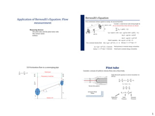
  • 1. 1 Application of Bernoulli’s Equation: Flow measurement Measuring devices: The pitot tube and the pitot-static tube The venturi meter Orifices Bernoulli’s Equation 𝑝 + 𝑑𝑝 𝐴 + 𝑑𝐴 𝑝𝐴 𝑑𝑠 𝜃 𝜌𝑔𝐴 𝑑𝑠 Force momentum relation applied to steady, 1D, inviscid fluid flow 𝑑𝑧 Consider a small stream tube having length ds For an inviscid flow, shear stresses are absent 𝐹𝑠𝑦𝑠 = 𝜌𝑄 𝑉2 − 𝑉1 − 𝑝 + 𝑑𝑝 𝐴 + 𝑑𝐴 + 𝑝𝐴 − 𝜌𝑔𝐴 𝑑𝑠 𝑆𝑖𝑛𝜃 = 𝜌𝑄 𝑉2 − 𝑉1 −𝑑𝑝 𝐴 − 𝜌𝑔𝐴 𝑑𝑧 = 𝜌𝑄 𝑑𝑉 −𝑑𝑝 𝐴 − 𝜌𝑔𝐴 𝑑𝑧 = 𝜌𝐴 𝑉 𝑑𝑉 𝑑𝑝 + 𝜌𝑔 𝑑𝑧 + 𝜌 𝑉 𝑑𝑉 = 0Euler’s equation For a constant density fluid 𝑑 𝑝 + 𝜌𝑔𝑧 + 𝜌𝑉2 /2 = 0 𝑑 𝑝/𝜌𝑔 + 𝑧 + 𝑉2 /2𝑔 = 0 𝑝 + 𝜌𝑔𝑧 + 𝜌𝑉2 /2 = 𝐶𝑜𝑛𝑠𝑡𝑎𝑛𝑡 𝑝/𝜌𝑔 + 𝑧 + 𝑉2 /2𝑔 = 𝐶𝑜𝑛𝑠𝑡𝑎𝑛𝑡 Total pressure is constant along a streamline Total head is constant along a streamline or 1D Frictionless flow in a converging pipe 𝜃 Datum z=0 Total head Piezometric head line 𝑃1 𝜌𝑔 𝑉1 2 2𝑔 𝑍1 𝑍2 𝑃2 𝜌𝑔 𝑉2 2 2𝑔 𝐴1 𝐴2 𝑃 𝜌𝑔 + 𝑧 + 𝑉2 2𝑔 = 𝐻 Consider a stream of uniform velocity flows into a blunt body Stream line pattern Apply Bernoulli equation to central streamline (1) and (2) 𝑃1 𝜌𝑔 + 𝑉1 2 2𝑔 + 𝑍1 = 𝑃2 𝜌𝑔 + 𝑉2 2 2𝑔 + 𝑍2 𝑉2 = 0; 𝑍1 = 𝑍2 𝑃1 𝜌𝑔 + 𝑉1 2 2𝑔 = 𝑃2 𝜌𝑔 𝑃2 = 𝑃1 + 1 2 𝜌𝑉1 2 Stagnation Pressure Static Pressure Dynamic Pressure Pitot tube
  • 2. 2 A piezometer and a pitot tube Two piezometers, one as normal and one as a Pitot tube within the pipe can be used in an arrangement shown below to measure velocity of flow 𝑃2 = 𝑃1 + 1 2 𝜌𝑉1 2 𝜌𝑔ℎ2 = 𝜌𝑔ℎ1 + 1 2 𝜌𝑉1 2 𝑉1 = 2𝑔 ℎ2 − ℎ1 Pitot tube 1 2 Pitot tube Pitot-static tube Close-up of a Pitot-static tube Pitot-static tube A pitot tube is connected to a manometer. The holes on the side of the tube connect to one side of a manometer and register the static head, (h1), while the central hole is connected to the other side of the manometer to register, as before, the stagnation head (h2). 1 2 𝜌𝑉1 2 = 𝜌𝑔ℎ − 𝜌 𝑚𝑎𝑛 𝑔ℎ 𝑉1 = 2𝑔ℎ 𝜌 𝜌 − 𝜌 𝑚 The Pitot/Pitot-static tubes give velocities at points in the flow Pitot-static tube (1) (1) (2) A B h x Connected point (1) Connected point (2) Consider the pressures on the level of the centre line of the Pitot tube 𝑃1 + 𝜌𝑔𝑥 = 𝑃2 + 𝜌𝑔(𝑥 − ℎ) + 𝜌 𝑚𝑎𝑛 𝑔ℎ 𝑃2 = 𝑃1 + 𝜌𝑔ℎ − 𝜌 𝑚𝑎𝑛 𝑔ℎ 𝑃2 = 𝑃1 + 1 2 𝜌𝑉1 2 Applying Bernoulli equation
  • 3. 3 Bernoulli equation: 𝑃1 𝜌𝑔 + 𝑉1 2 2𝑔 + 𝑍1 = 𝑃2 𝜌𝑔 + 𝑉2 2 2𝑔 + 𝑍2 Carefully designed to minimize the energy losses Converging section: 𝒅𝒑 𝒅𝒙 < 𝟎 Favorable pressure gradient, Stable flow, negligible energy loss Diverging section: 𝒅𝒑 𝒅𝒙 > 0 Adverse pressure gradient: Unstable flow, energy loss Converging section (1) (2) Δh h2=P2/ρg h1=P1/ρg 𝑃1 𝜌𝑔 + 𝑧1 − 𝑃2 𝜌𝑔 + 𝑧2 = 𝑉2 2 2𝑔 − 𝑉1 2 2𝑔 ∆ℎ = 𝑄2 2𝑔 1 𝐴2 2 − 1 𝐴1 2 𝑄 = 𝐴1 𝐴2 2𝑔∆ℎ 𝐴1 2 − 𝐴2 2 Continuity equation: 𝑄 = 𝐴1 𝑉1 = 𝐴2 𝑉2; 𝐴2 < 𝐴1; 𝑉2 > 𝑉1 ; 𝑉1 = 𝐴2 2𝑔∆ℎ 𝐴1 2 − 𝐴2 2 Constriction flow meters Orifice meter Flow nozzle Venturi meter Constriction flow meters In terms of the manometer readings 𝑃1 + 𝜌𝑔𝑍1 = 𝑃2 + 𝜌𝑔(𝑍2 − ℎ) + 𝜌 𝑚𝑎𝑛 𝑔ℎ 𝑃1 − 𝑃2 𝜌𝑔 + 𝑍1 − 𝑍2 = ℎ 𝜌 𝑚𝑎𝑛 𝜌 − 1 𝑉1 = 𝐴2 2𝑔 𝑃1 − 𝑃2 𝜌𝑔 + 𝑍1 − 𝑍2 𝐴1 2 − 𝐴2 2 𝑉1 = 𝐴2 2𝑔ℎ 𝜌 𝑚𝑎𝑛 𝜌 − 1 𝐴1 2 − 𝐴2 2 𝑄 𝑎𝑐𝑡 = 𝐶 𝑑 𝐴1 𝐴2 2𝑔ℎ 𝜌 𝑚𝑎𝑛 𝜌 − 1 𝐴1 2 − 𝐴2 2 Venturi meter About 200 About 60 Z2 Z1 h Datum Streamline pattern Orifice meter RoundedSharp-edge Square shoulder Thick-plate square edge Orifice in a pipe
  • 4. 4 ‘small orifice’: orifice diameter is small compared to head producing flow (head does not vary across the orifice) h P0 (1) (2) 0 open to atm 0 Tank is large 0 Torricelli’s theorem: Velocity of a issuing jet is proportional to the square root of the head producing flow Liquid flow Small orifice Applying Bernoulli’s equation to (1) and 2) 𝑃1 𝜌𝑔 + 𝑍1 + 𝑉1 2 2𝑔 = 𝑃2 𝜌𝑔 + 𝑍2 + 𝑉2 2 2𝑔 𝑉2 = 2𝑔ℎ ; 𝑄 = 𝑎 2𝑔ℎ Vena Contractor Actual area Vena Contractor Actual area In practice, actual discharge is less than the theoretical discharge Reasons: Actual velocity <Theoretical velocity due to energy loss between (1) and (2) 𝑉𝑎𝑐𝑡 = 𝐶 𝑣 2𝑔ℎ 𝐶𝑣− coefficient of velocity Fluid path converges on the orifice. Area is less than the orifice area 𝐴 𝑎𝑐𝑡 = 𝐶𝑐 𝐴 𝑜𝑟𝑖𝑓𝑖𝑐𝑒; 𝐶𝑐- coefficient of contraction 𝑄 𝑎𝑐𝑡 = 𝐶𝑣 2𝑔ℎ . 𝐶𝑐 𝐴 𝑜𝑟𝑖𝑓𝑖𝑐𝑒 𝑄 𝑎𝑐𝑡 = 𝐶𝑣 2𝑔ℎ . 𝐶𝑐 𝐴 𝑜𝑟𝑖𝑓𝑖𝑐𝑒 Coefficient of discharge 𝐶 𝑑 = 𝐶𝑐 𝐶 𝑣 Coefficient of discharge depends on the edge condition 𝐶𝑐 ≈ 1 𝐶𝑣 ≈ 0.98 𝐶 𝑑 ≈ 0.98 𝐶𝑐 ≈ 1 𝐶𝑣 ≈ 0.86 𝐶 𝑑 ≈ 0.86 𝐶𝑐 ≈ 0.62 𝐶𝑣 ≈ 0.98 𝐶 𝑑 ≈ 0.61 𝐶𝑐 ≈ 0.62 𝐶𝑣 ≈ 0.98 𝐶 𝑑 ≈ 0.61 *Contraction of jet RoundedSharp-edge Square shoulder Thick-plate square edge Determination of the coefficient of contraction, velocity, and discharge (Cc , Cv , and Cd) x y H 𝑢 𝑡ℎ𝑒𝑜𝑟𝑒𝑡𝑖𝑐𝑎𝑙 = 2𝑔𝐻 𝑈𝐴 = 𝐶𝑣 𝑉𝑇 𝐶𝑣 = 𝑔 2𝑦 𝑥 2𝑔𝐻 𝐶𝑣 = 𝑥2 4𝑦𝐻 𝐶 𝑑 = 𝑄 𝐴 𝑄 𝑇 𝑄 𝑇 = a 2𝑔ℎ 𝑄 𝐴 √ Use direct method 𝐶𝑐 = 𝐶 𝑑 𝐶𝑣 𝑥 = 𝑢𝑡; 𝑡 = 𝑥 𝑢 𝑦 = 1 2 𝑔𝑡2 𝑢 = 𝑔 2𝑦 𝑥
  • 5. 5 Falling head method: Determine coefficient of discharge (For any outflow device) 𝑄 = 𝐴𝑉 𝑄 = 𝐴 𝑑ℎ 𝑑𝑡 A 𝑑ℎ 𝑑𝑡 = 𝑄𝑖𝑛 − 𝑄 𝑜𝑢𝑡 𝑄𝑖𝑛=0; 𝑄 𝑜𝑢𝑡 = 𝐶 𝑑 𝑎 2𝑔𝐻 for small orifice A 𝑑ℎ 𝑑𝑡 = −𝐶 𝑑 𝑎 2𝑔𝐻 𝑑𝑡 = − 𝐴 𝐶 𝑑 𝑎 2𝑔 𝑑 𝑑ℎ ℎ0.5 𝑡 = − 2𝐴 𝐶 𝑑 𝑎 2𝑔 𝑑 ℎ0.5 + 𝐶 𝑡 = 0;ℎ = ℎ1 𝑡 = 𝑇; ℎ = ℎ2 𝑇 = 2𝐴 𝐶 𝑑 𝑎 2𝑔 ℎ1 0.5 − ℎ2 0.5 h1 h2 Area A Orifice area =a Exercise A large tank contains a liquid to a depth z. A small orifice located at height y above the tank base discharges a horizontal jet to the atmosphere. The jet strikes the base level of the tank at a horizontal distance x. Assume 𝐶𝑣 = 1 , 𝐶𝑐 = 0.63, 𝐴 = 670𝑎 (i) Show that 𝑥2 + 4𝑦2 = 4𝑦𝑧 and that the maximum horizontal distance occurs when 𝑧 = 2𝑦 (ii) Given y=0.25 m, find the time taken for the jet striking distance x to change from 𝑥1 = 1𝑚 to 𝑥2 = 0.5𝑚 h1 h2 x y z Exercise: Approach velocity (𝑽 𝟎) correction H=2.5 m P0 (0) (1) Liquid flow Area: A Area: a 𝑃0 𝜌𝑔 + 𝑍0 + 𝑉0 2 2𝑔 = 𝑃1 𝜌𝑔 + 𝑍1 + 𝑉1 2 2𝑔 𝑍0 + 𝑉0 2 2𝑔 =𝑍1 + 𝑉1 2 2𝑔 𝑉0 2 2𝑔 + 𝐻= 𝑉1 2 2𝑔 𝐴0 𝑉0 = 𝐴1 𝑉1 Applying continuity equation: 𝑉0 = 𝑎 𝐴 𝑉1 𝑎 𝐴 2 𝑉1 2 2𝑔 + 𝐻= 𝑉1 2 2𝑔 𝑉 = 2𝑔𝐻 1 − 𝑎2 𝐴2 A/a V 5 ? 10 ? 100 ? 1000 ? 𝑉 = 2𝑔𝐻 = 7 𝑚/𝑠 Assumed small area; if orifice area is not small h1 h2 𝑉1 = 2𝑔ℎ1 𝑉2 = 2𝑔ℎ2 Velocity will change across the orifice Head vary substantially from top to bottom
  • 6. 6 For small area dA; 𝑉 = 2𝑔ℎ 𝑑𝑄 = 𝑏𝑑ℎ 2𝑔ℎ Large rectangular orifice: vertical height is large h1 h2 h dh *Side contraction Integrate over area; 𝑄 = 𝑏 2𝑔 ℎ. 𝑑ℎ ℎ2 ℎ1 𝑄 = 𝐶 𝑑 2𝑏 3 2𝑔 ℎ2 3/2 − ℎ1 3/2 Notches and weirs Notch: Opening in the side of a tank or reservoir, extending above the free surface (No upper edge) Weir: notch on a large scale, to measure the flow of a river Rectangular notch b H h 𝑄 = 𝐶 𝑑 2𝑏 3 2𝑔 𝐻3/2 𝑄 = 𝐶 𝑑 2𝑏 3 2𝑔 ℎ2 3/2 − ℎ1 3/2 0 𝑑𝐴 = 2 𝐻 − ℎ 𝑇𝑎𝑛𝜃. 𝑑ℎ 𝑑𝑄 = 2𝑔ℎ .2 𝐻 − ℎ 𝑇𝑎𝑛𝜃. 𝑑ℎ 𝑑𝑄 = 2 2𝑔 𝑡𝑎𝑛𝜃. ℎ1/2 𝐻 − ℎ 𝐻 0 𝑑ℎ 𝑄 𝑎𝑐𝑡 = 𝐶 𝑑 8 15 2𝑔 𝑡𝑎𝑛𝜃 𝐻5/2 Vee notch H h Weir Calibration For a V notch: Applying mass continuity equation (assume quasi steady condition) 𝐴 𝑑𝐻 𝑑𝑡 = 𝑄𝑖𝑛 − 𝑄 𝑜𝑢𝑡 = 0 − 𝐶 𝑑 8 15 2𝑔 𝑡𝑎𝑛𝜃 𝐻 5 2 Integrating: 𝑇 = 5𝐴 4𝐶 𝑑 𝐻2 −3/2 − 𝐻1 −3/2 𝑡𝑎𝑛𝜃 2𝑔
  • 7. 7 Angular momentum equation Moment of momentum equation For a particle dm having velocity 𝑉 ; Linear momentum = 𝑉.dm Moment about axis on O = 𝑟 x 𝑉.dm 𝐻0 = 𝑟 x 𝑉.dm 𝑠𝑦𝑠 H- moment of momentum 𝑉𝑡 𝑇𝑟𝑒𝑛𝑠𝑣𝑒𝑟𝑠𝑒 𝑡𝑎𝑛𝑔𝑒𝑛𝑡𝑖𝑎𝑙 𝑣𝑒𝑙𝑜𝑐𝑖𝑡𝑦 𝑉𝑟 𝑅𝑎𝑑𝑖𝑎𝑙 𝑣𝑒𝑙𝑜𝑐𝑖𝑡𝑦 Moment of momentum Angular momentum equation Newton’s 2nd law to rotating systems: 𝐹 = 𝑑 𝑑𝑡 𝑚𝑉 𝑟x 𝐹 = 𝑟 𝑑 𝑑𝑡 𝑚𝑉 𝑟x 𝐹 = 𝑑 𝑑𝑡 𝑟 × 𝑚 𝑉 𝑇 = 𝑑𝐻 𝑑𝑡 T net torque or moment applied on the system Rate of change of moment of momentum (angular momentum) of a system is equal to the net torque acting on the system Angular momentum equation-CV Expression 𝐻0 = 𝑟 x 𝑉.dm 𝑠𝑦𝑠 𝑇 = 𝑑𝐻 𝑑𝑡 Newton’s 2nd law to rotating systems 𝑑𝐵𝑠𝑦𝑠 𝑑𝑡 = 𝜕 𝜕𝑡 𝛽𝜌𝑑∀ 𝐶𝑉 + 𝛽 𝐶𝑆 𝜌𝑉. 𝑑𝐴 For a stationary CV, RTT 𝑑𝐵 = 𝛽. 𝑑𝑚 = 𝛽. 𝜌. 𝑑∀ 𝐵 = 𝛽. 𝜌. 𝑑∀ 𝐶𝑉 Extensive property B = moment of momentum 𝐵 = 𝑟 x 𝑉.dm = 𝑟 x 𝑉.ρ𝑑∀𝐶𝑉𝐶𝑉 𝛽 = 𝑑𝐵 𝑑𝑚 = 𝑑𝐻0 𝑑𝑚 = 𝑟 x 𝑉 CV expression for angular momentum equation 𝑑𝐻 𝑠𝑦𝑠 𝑑𝑡 = 𝜕 𝜕𝑡 𝑟x 𝑉𝜌𝑑∀𝐶𝑉 + 𝑟 × 𝑉𝐶𝑆 𝜌𝑉. 𝑑𝐴 𝑇 = 𝑑𝐻 𝑑𝑡 𝐶𝑉 + 𝐻 𝑜 𝑜𝑢𝑡 -𝐻 𝑜 𝑖𝑛 Angular momentum equation-CV Expression Cont. Steady flow 𝑑𝐻 𝑑𝑡 𝐶𝑉 =0 ; 𝑇 = 𝐻 𝑜 𝑜𝑢𝑡 −𝐻 𝑜 𝑖𝑛 = (𝑟 × 𝑉𝑚) 𝑜𝑢𝑡- (𝑟 × 𝑉𝑚)𝑖𝑛 Steady 1D flow: 𝑇 = ρ𝑄 𝑟2 𝑉2 − 𝑟1 𝑉1 The sum of all external moments acting on a CV The rate of change of the angular momentum of the contents of the CV The net rate of angular momentum out of the control surface = + 𝑇 = 𝑑𝐻 𝑑𝑡 𝐶𝑉 + 𝐻 𝑜 𝑜𝑢𝑡 -𝐻 𝑜 𝑖𝑛
  • 8. 8 Application Pump 𝑇 = ρ𝑄 𝑟2 𝑉2 − 𝑟1 𝑉1 Fluid EnergyMechanical Energy Centrifugal Pump Flow direction Vt2 Vt1 r2 r1 ω Example 1 20 cm 30 cm A Bω A sprinkler with two nozzles of diameter 4 mm each is connected across a tap of water. The nozzles are at a distance of 30 cm and 20 cm from the centre of the tap. The flow rate of water through tap is 120 cm3/s. The nozzles discharge water in the downward direction. Determine the angular speed at which the sprinkler will rotate free. 2- arm rotating sprinkler 𝜃 Datum z=0 Total head Piezometric head line 𝑃1 𝜌𝑔 𝑉1 2 2𝑔 𝑍1 𝑍2 𝑃2 𝜌𝑔 𝑉2 2 2𝑔 𝐴1 𝐴2 𝑃 𝜌𝑔 + 𝑧 + 𝑉2 2𝑔 = 𝐻 𝑃1 𝜌𝑔 + 𝑍1 + 𝑉1 2 2𝑔 = 𝑃2 𝜌𝑔 + 𝑍2 + 𝑉2 2 2𝑔 Consider a streamline between two points 1 and 2 Bernoulli equation Modifications of Bernoulli Equation In practice, the total energy of a streamline does not remain constant Consider a streamline between two points 1 and 2 𝐻1 + 𝐻𝑒𝑎𝑑 𝑎𝑑𝑑𝑖𝑡𝑖𝑜𝑛𝑠 − 𝐻𝑒𝑎𝑑 𝑙𝑜𝑠𝑠𝑒𝑠 = 𝐻2 Head balance equation 𝐻1 ∓ 𝐻 𝐸 − 𝐻𝑓 = 𝐻2 𝑃1 𝜌𝑔 + 𝑉1 2 2𝑔 + 𝑍1 ∓ 𝐻 𝐸 − 𝐻𝑓 = 𝑃2 𝜌𝑔 + 𝑉2 2 2𝑔 + 𝑍2 (3.12) Energy is ‘lost’ through friction (actually transformed into heat), and external energy may be either added by means of a pump or extracted by a turbine 𝜃𝐴1 𝐴2 Losses (transformed into another state) Additions
  • 9. 9 ℎ 𝑓 = 𝜆 𝐿 𝐷 𝑉2 2𝑔 L (m) to to (N/m2) to to v (m/s) P1 (N/m2) P2 (N/m2) 1 2 D (m) Head loss due to friction If the flow is inviscid ℎ 𝑓 = 0 The effect of friction on layers of water molecules Viscosity: measure of a fluid's resistance to flow Sudden Expansion Sudden Contraction The flow is not able to follow the shape. As a result, there is flow separation, creating turbulent eddies. Minor loss: energy loss due to obstructions hL=K . (v2 2/2g) hL=K . (v1 2/2g) hL=KL . (v2 2/2g)Entrance losses: Minor loss: energy loss due to obstructions hL=KL . (v1 2/2g)Exit losses: Minor loss: energy loss due to obstructions
  • 10. 10 Minor loss: energy loss due to obstructions A divergent duct or diffuser Tee junctions Bends Y junctions P = power added to fluid 𝑃 = 𝜌𝑔 𝑄 𝐻 𝐸 Pumps add energy to the flow Mechanical Energy Fluid Energy Centrifugal Pump Turbines extracts energy from the flow Mechanical Energy Fluid Energy Pelton Wheel Impeller Buckets Inlet Nozzle Spear Discharge Deflector plate 2 2 V g 2 2 V g p g Representation of energy terms 2 2 V g p g wh wh wh 2 2V g p g 2 2 V g p g Representation of energy terms
  • 11. 11 Conservation of Energy 𝑑𝐸𝑆 𝑑𝑡 = 𝐻𝑡 + 𝑊𝑘 Rate of change of energy of a system Net rate of heat transfer Net power (rate of work) input to the system Energy (E) = kinetic energy+ potential energy+ internal energy (related to molecularmotion) = 1 2 𝑚𝑉2 + 𝑚𝑔𝑍 + 𝑚𝑖 Specific energy (e )= 1 2 𝑉2 + 𝑔𝑍 + 𝑖 Incompressible fluids with constant temperature: 𝑑𝐸 𝑆 𝑑𝑡 = 𝑊𝑘 E = 1 2 𝑚𝑉2 + 𝑚𝑔𝑍; e = 1 2 𝑉2 + 𝑔𝑍 In the analysis of fluid flow systems: 𝑬 𝟏 + 𝑬𝒏𝒆𝒓𝒈𝒚 𝒂𝒅𝒅𝒊𝒕𝒊𝒐𝒏𝒔 − 𝑬𝒏𝒆𝒓𝒈𝒚 𝒍𝒐𝒔𝒔𝒆𝒔 = 𝑬 𝟐 𝑬 𝟏 − 𝑬 𝟐 = 𝑬𝒏𝒆𝒓𝒈𝒚 𝒂𝒅𝒅𝒊𝒕𝒊𝒐𝒏𝒔 − 𝑬𝒏𝒆𝒓𝒈𝒚 𝒍𝒐𝒔𝒔𝒆𝒔 𝒅𝑬 = 𝑬𝒏𝒆𝒓𝒈𝒚 𝒂𝒅𝒅𝒊𝒕𝒊𝒐𝒏𝒔 − 𝑬𝒏𝒆𝒓𝒈𝒚 𝒍𝒐𝒔𝒔𝒆𝒔 Internal energy: Energy due to molecular motion in a fluid, depends on the temperature and physical state (liquid, gas, two phase) 𝜃𝐴1 𝐴2 𝐸1 𝐻1 𝐸2 𝐻2 Losses Additions Work associated with force acting through a distance 𝑊𝑇𝑜𝑡𝑎𝑙 = 𝑊𝑠ℎ𝑎𝑓𝑡 + 𝑊𝑝𝑟𝑒𝑠𝑠𝑢𝑟𝑒 + 𝑊𝑣𝑖𝑠𝑐𝑜𝑢𝑠 𝑊𝑠ℎ𝑎𝑓𝑡- work transmitted by a rotating shaft (Turbine, pumps) 𝑊𝑝𝑟𝑒𝑠𝑠𝑢𝑟𝑒-work done by the pressure forces on the control surface 𝑊𝑣𝑖𝑠𝑐𝑜𝑢𝑠- normal and shear components of the viscous forces on the control surface Note: not considered if the moving walls are inside the control volume and fixed walls are outside the control volume 𝑊𝑇𝑜𝑡𝑎𝑙 = 𝑊𝑠ℎ𝑎𝑓𝑡 + 𝑊𝑝𝑟𝑒𝑠𝑠𝑢𝑟𝑒 Power transmitted through rotating shaft 𝑊𝑠ℎ𝑎𝑓𝑡 = 𝜌𝑔𝑄𝐻 = 𝜔𝑇𝑠ℎ𝑎𝑓𝑡 = 2𝜋𝑛 𝑇𝑠ℎ𝑎𝑓𝑡 𝜔 –angular speed of shaft (rad/s) 𝑇𝑠ℎ𝑎𝑓𝑡-Shaft torque 𝑛 - number of revolutions of the shaft per unit time (rpm) Work done by the pressure=Force x Distance travelled = 𝑃𝐴 × 𝑚 𝜌 𝐴 = 𝑃 × 𝑚 𝜌 Incompressible fluids with constant temperature: 𝑑𝐸𝑆 𝑑𝑡 = 𝑊𝑘 = 𝑊𝑠ℎ𝑎𝑓𝑡 + 𝑊𝑝𝑟𝑒𝑠𝑠𝑢𝑟𝑒 E = 1 2 𝑚𝑉2 + 𝑚𝑔𝑍; e = 1 2 𝑉2 + 𝑔𝑍 𝑑𝐵𝑠𝑦𝑠 𝑑𝑡 = 𝜕𝐵𝑐 𝜕𝑡 + 𝐵 𝑜𝑢𝑡 − 𝐵𝑖𝑛 = 𝜕 𝜕𝑡 𝛽𝜌𝑑∀ 𝐶𝑉 + 𝛽 𝐶𝑆 𝜌𝑉. 𝑑𝐴 B: Energy (E) 𝑑𝐸𝑠𝑦𝑠 𝑑𝑡 = 𝜕𝐸𝑐 𝜕𝑡 + 𝐸 𝑜𝑢𝑡 − 𝐸𝑖𝑛 = 𝜕 𝜕𝑡 𝑒𝜌𝑑∀ 𝐶𝑉 + 𝑒 𝐶𝑆 𝜌𝑉. 𝑑𝐴 β: Energy (E)/unit mass = e RTT; 𝑆𝑡𝑒𝑎𝑑𝑦 1𝐷 𝑓𝑙𝑜𝑤 ; 𝜕𝐸 𝑐 𝜕𝑡 = 0 𝑑𝐸𝑠𝑦𝑠 𝑑𝑡 = 𝐸 𝑜𝑢𝑡 − 𝐸𝑖𝑛 = 𝑒 𝐶𝑆 𝜌𝑉. 𝑑𝐴 𝑑𝐸𝑠𝑦𝑠 𝑑𝑡 = ( 1 2 𝑚 𝑉2 + 𝑚 𝑔𝑍 + 𝑃 𝑚 𝜌 ) 𝑜𝑢𝑡−( 1 2 𝑚 𝑉2 + 𝑚 𝑔𝑍 + 𝑃 𝑚 𝜌 )𝑖𝑛= ( 1 2 𝑉2 + 𝑔𝑍 + 𝑃 𝑚 𝜌 ) 𝐶𝑆 𝜌𝑉. 𝑑𝐴 𝑊𝑠ℎ𝑎𝑓𝑡/𝑚 𝑔 = ( 𝑉2 2𝑔 + 𝑍 + 𝑃 𝜌𝑔 ) 𝑜𝑢𝑡−( 𝑉2 2𝑔 + 𝑍 + 𝑃 𝜌𝑔 )𝑖𝑛 𝑊𝑠ℎ𝑎𝑓𝑡 𝑚 𝑔 = 2𝜋𝑛 𝑇𝑠ℎ𝑎𝑓𝑡 𝑚 𝑔 = 𝜌𝑔𝑄𝐻 𝑚 𝑔 = 𝐻 𝑊𝑠ℎ𝑎𝑓𝑡/𝑚 𝑔 = ( 𝑉2 2𝑔 + 𝑍 + 𝑃 𝜌𝑔 ) 𝑜𝑢𝑡−( 𝑉2 2𝑔 + 𝑍 + 𝑃 𝜌𝑔 )𝑖𝑛 𝐻 𝐸 = ( 𝑉2 2𝑔 + 𝑍 + 𝑃 𝜌𝑔 ) 𝑜𝑢𝑡−( 𝑉2 2𝑔 + 𝑍 + 𝑃 𝜌𝑔 )𝑖𝑛
  • 12. 12 A large closed tank contains a liquid of density 850 kg/m3 and air is under pressure of 25 kPa. The liquid is discharged to the atmosphere at N through nozzle of diameter 60 mm located at the end of pipe of diameter 120 mm fitted with a pump as shown in the Figure. The head loss in the pipe AP (suction pipe) is 6 𝑉2 2𝑔 and the head loss in the pipe PM (delivery pipe) is 4 𝑉2 2𝑔 where V is the velocity in pipes JP and PM. The head loss in nozzle MN is negligible. Find the power required by the pump to deliver 25 l/s. Draw the total head line clearly indicating magnitudes of changes in head. Find the discharge, if the head added by the pump drops by 50 %. M Water is pumped from reservoir A to reservoir B through a pipe with the highest point C at a flow of 60 l/s. The diameter of the pipe is 0.2 m. The atmospheric pressure is 10 m water. The head losses hL between C and B are 2.8 m. To what highest elevation at point C can the pipe reach if the absolute pressure has to be at least 2 m of water. pump A B C +15 +30 20 m 300 m 100 m A large open tank contains an oil of density 850 kg/m3. The oil is discharged to the atmosphere at K through a pipeline fitted with a pump at P. The head loss in the 150 mm diameter pipe JP is 2 𝑉1 2 2𝑔 and the head loss in the 100 mm diameter pipe PK is 3 𝑉2 2 2𝑔 where V1 and V2 are the velocities in pipes JP and PK, respectively. a) When the pump adds 5 kW of power causing a discharge of 60 l/s at K, find the elevation h at K and the deflection δ of the mercury manometer What is the volume flow rate through the pipe if the pump is removed? A large closed tank contains a liquid of density 850 kg/m3 and air is under pressure P0. The liquid is discharged to the atmosphere through a pipeline fitted with a pump. The head loss in the 300 mm diameter pipe JM is 9 𝑉2 2𝑔 .The head loss in pipe MN is negligible. For Q= 140 l/s, find P0 when the pump is not working.
  • 13. 13 A large open tank contains an oil of density 850 kg/m3. The tank is discharged to the atmosphere at K through a pipeline fitted with a pump at P as shown in figure. The head loss in the 150 mm diameter pipe JP is 2 𝑉1 2 2𝑔 and the head loss in the 100 mm diameter pipe PK is 3 𝑉2 2 2𝑔 where V1 and V2 are the velocities in pipes JP and PK, respectively.