Build a radio telescope with RAL10AP (by RadioAstroLab).

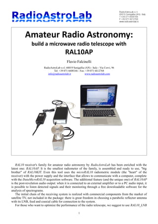
1. Amateur Radio Astronomy:
build a microwave radio telescope with
RAL10AP
Flavio Falcinelli
RadioAstroLab s.r.l. 60019 Senigallia (AN) - Italy - Via Corvi, 96
Tel: +39 071 6608166 - Fax: +39 071 6612768
info@radioastrolab.it www.radioastrolab.com
RAL10 receiver's family for amateur radio astronomy by RadioAstroLab has been enriched with the
latest one: RAL10AP. It is the smallest radiometer of the family, is assembled and ready to use, "big
brother" of RAL10KIT. Even this tool uses the microRAL10 radiometric module (the "heart" of the
receiver) with the power supply and the interface that allows to communicate with a computer, complete
with the DataMicroRAL10 acquisition software. The additional feature (and the unique one) of RAL10AP
is the post-revelation audio output: when it is connected to an external amplifier or to a PC audio input, it
is possible to listen detected signals and their monitoring through a free downloadable software for the
analysis of spectrograms.
The initial chain of the receiving system is realized with commercial components from the market of
satellite TV, not included in the package: there is great freedom in choosing a parabolic reflector antenna
with its LNB, feed and coaxial cable for connection to the system.
For those who want to optimize the performance of the radio telescope, we suggest to use RAL10_LNB
1

2. thermally controlled outdoor unit and the RAL230ANT antenna, a satellite dish of 2.3 meters in diameter,
the outdoor unit can be easily installed on equatorial mounts commonly used for astronomical optical
observations or on antenna handling systems used by radio amateurs. The experimenter will be able to
customize and optimize his radio astronomy station, our catalog includes all necessary accessories.
RadioAstroLab offers also a consulting service and an "ad hoc" production of tools for amateur radio
astronomy and for scientific applications in general. The consulting can range from modifications or
specific customizations requested by customers, to the design and production of radio astronomy
complete systems and amateur and semi-professional radio telescopes. This service is offered to requests
by private individuals, but also to those ones of groups (such as, for example, amaterur astronomers and
radio amateurs), of scientific working groups, of schools and universities, of government and private
research institutions, of museums and science institutes, these kind of organizations often ask customized
solutions.
In this document we describe the way for using RAL10AP to build a radio telescope which is the first
approach to radio astronomy.
Introduction
The construction of simple and inexpensive microwave radio telescopes, operating in 10-12 GHz
frequency band, is now greatly simplified if you use antenna systems and components from the market of
satellite TV, available everywhere at low cost. A similar instrument enables a simple and immediate
approach to radio astronomy and acquisitions basic techniques and interpretations of measures. Thanks to
the commercial deployment of the satellite TV service are readily available modules such as low noise
preamplifiers-converters (LNB: Low Noise Block) and IF preamplifiers line. In this wide range of
products are included parabolic reflectors antennas available in various sizes, complete with mechanical
support for the assembly and orientation.
Using a common TV-SAT antenna with its specific LNB outdoor unit (with feed) and connecting these
ones to RAL10AP, you can build a radiometer operating at 11.2 GHz for the study of the thermal radiation
of the Sun, Moon, and more intense radio sources, with sensitivity mainly function of the size of the
antenna used. It is a complete tool which also provides the USB interface for communication with a PC
station, the detected signal audio output and the DataMicroRAL10 software for the automatic acquisition
of data and for control of the receiver. The user only needs to connect the components according to the
instructions supplied, to provide a power source and assemble the system in an enclosure: the telescope is
ready to begin the observations. The construction and development of this tool could be tackled
successfully by students, radio amateur and radio astronomy enthusiasts, getting results more interesting
as the larger the antenna used and the more “fancy” and expertise is used to expand and refining its basic
performance.
Due to the short wavelength, it is relatively simple to build amateur radio telescopes with good
features and acceptable resolution. Although in this frequency range is not “shine” particularly intense
radio sources (excluding the Sun and the Moon), the sensitivity of the system is enhanced by the large
bandwidth used and the reduced influence of artificial disturbances: the radio telescope can be installed
on the roof or the garden of the house in an urban area. Television geostationary satellites can be
interference sources, you can avoid them without limiting the scope of observation, since their position is
fixed and known. As we'll see, the ability to monitor the detected audio signal using any one of the
downloaded free programs for the spectrograms analysis, allows you to check the presence of interfering
radio signals of artificial origin.
For its economy and practicality RAL10AP represents the best starting point for fans who want to
approach the world of amateur astronomy observing the sky with a different approach compared to the
traditional one.
2

3. The receiver: how works a Total-Power radiometer.
The radiometer is a microwave receiver very sensitive and calibrated, used to measure the temperature
associated to the scenario intercepted by the antenna, since any natural object emits a noise power
function of the temperature and of the physical characteristics.
In radiometry is convenient to express the power in terms of equivalent temperature: according to the
Rayleigh-Jeans law, which applies at microwave frequencies, it is always possible to determine a
temperature of a black body (called brightness temperature) that radiates the same power of the energy
dissipated by a terminating resistor connected to the receiving antenna (antenna temperature).
Considering an ideal antenna “seeing” an object characterized by a given brightness temperature, one can
express the measured signal power from the antenna is expressible with the antenna temperature.
Objective of the radiometric measurement is to derive the brightness temperature of the object from the
antenna temperature with sufficient resolution and accuracy.
Fig. 1: Sky brightness temperature as a function of frequency and of the elevation angle of the antenna.
In radioastronomy the received signal is proportional to the power associated to the radiation
mediated within the passband of the instrument, then the brightness temperature of the region of sky
“seen” by the antenna beam. The radiometer behaves like a thermometer that measures the equivalent
noise temperature of the observed celestial scenario. Our radio telescope, operating at 11.2 GHz
frequency, detects a temperature of very low noise (due to the fossil radiation approximately 3 K),
generally in the order of 6-10 K (the cold sky) which corresponds to the lowest temperature measurable
from the instrument and takes into account the instrumental losses (Fig.1), if the antenna is oriented
towards a region of clear and dry sky, where radio sources are absent (clear atmosphere, with negligible
atmospheric absorption - Fig. 2). If the orientation of the antenna is kept at 15°-20° above the horizon,
away from the Sun and the Moon, we can assume an antenna temperature between a few degrees and a
3

4. few tens of degrees (mainly due to the secondary lobes). Pointing the antenna on the ground the
temperature rises to values of the order of 300 K, if it is interested in all the received beam.
Fig. 2: Attenuation due to the absorption properties of the gas present in the atmosphere.
The most simple microwave radiometer (Fig.3) comprises an antenna connected to a low noise
amplifier (LNA: Low Noise Amplifier) followed by a detector with quadratic characteristic. The “useful
information in radio astronomy” is the power associated with the received signal, proportional to its
square: the device which provides this function is the detector, generally implemented with a diode
operating in the region of its characteristic curve with the quadratic response. To reduce the contribution
of the statistical fluctuations of the noise revealed, and then optimize the sensitivity of the receiving
system, follows an integrator block (low-pass filter) that calculates the time average of the detected signal
according to a given time constant.
The radiometer just described is called Total-Power receiver because it measures the total power
associated with the signal received by the antenna and the noise generated by the system. The signal
output of the integrator appears as a quasi-continuous component due to the noise contribution of the
system with small variations (of amplitude much less than that of the stationary component) due to the
radio sources that “transit” before the antenna beam. Using a differential circuit of post-detection, if
receiver's parameters are stable, it is possible to measure only the power changes due to the radiation
4

5. coming from the object “framed” by the receive beam, “erasing” the quasi-continuous component due to
noise of the receiving system: this is the purpose of the reset signal of the baseline shown in Fig. 3.
The main problem of the radioastronomical observations is related to the instability amplification
factor of receiver with respect to temperature changes: you can observe drifts on quasi-continuous
component revealed that “confuse” the instrument, partially canceling the compensation action of the
base line. Such fluctuations are indistinguishable from “useful variations” of the signal. If the receiving
chain amplifies greatly, due to instability, it is easy to observe fluctuations in the output signal such as to
constitute a practical limit to the maximum value used for amplification. This problem can be partially
solved, with satisfactory results in amateur applications, thermally stabilizing the receiver and the outdoor
unit (LNB: Low Noise Block) located on the antenna focus and more subject to daily temperature.
Specially designed for this purpose is the RAL10_LNB unit, available on request: the device, installed on
the antenna's focus, can be connected via TV-SAT coaxial cable to all the receivers of RAL10 family. The
unit, built in a robust aluminum insulated case, is thermally stabilized with an internal regulator: an
electric cable (separate from the coaxial cable) supply the low voltage power (12 V) for the stabilization
circuit. The user can choose to power the thermal stabilization circuit when observations require high
accuracy.
Fig. 3: Simplified block diagram of a Total-Power radiometer.
We describe briefly the characteristics of the radiometric module that is the core of the system. Figure
4 shows a block diagram of the radio telescope with RAL10AP. For simplicity the power supply and post-
revelation output audio circuit are not shown. You can see the three main sections of the receiver: the first
one is the LNB (Low Noise Block) that amplifies the received signal and converts it down in the standard
IF frequency band [950-2150] MHz of TV satellite reception. This device is a commercial product,
usually supplied with the antenna and the mechanical supports needed for assembly. The power gain of
the unit is of the order of 50-60 dB, with a typical noise variable between 0.3 and 1 dB. For those who
want to optimize the radio telescope performances, we suggest to use the RAL10_LNB outdoor unit,
equipped with an automatic control that stabilizes the internal temperature.
The signal at the intermediate frequency (IF) is applied to the radiometric module that provides
filtering (with a bandwidth of 50 MHz, centered at the frequency of 1415 MHz), amplifies and measures
received signal power. It is available an auxiliary audio output, useful for monitoring the characteristics of
the detected signal: this signal, applied to the input audio of a PC, can be amplified and listened, as well
as studied in the frequency domain, using one of the many free programs downloadable software for the
analysis of spectrograms. Since the audio output is taken after the post-detection amplifier, its level
depends on the level of the base line radiometric calibration. Fig. 9 shows an example of audio output use
5

6. (not exactly radio astronomy, but useful for identifying potential artificial interferences). This
characteristic is a specific feature of RAL10AP.
A post-detection amplifier adjusts the level of the detected signal to the dynamics of acquisition of the
analog-digital converter (ADC with 14 bit resolution) that “digitizes” the radiometric information. This
final block, managed by a microcontroller, generates a programmable offset for the radiometric baseline
(the signal Vref in Fig. 3), calculates the moving average of an established number of samples and forms
the packet of serial data that will be transmitted to the central unit. The last stage is the USB interface that
manages communication with the PC on which the DataMicroRAL10 software will be installed for the
acquisition and instrument control. The processor executes the critical functions of processing and control
minimizing the number of external electronic components and maximizing the flexibility of the system
due to the possibility to schedule the operating parameters of the instrument. The use of a module
specifically designed for radio astronomy observations, which integrates all the functionality of a
radiometric receiver, ensures the experimenter safe and repeatable performances.
Fig. 4: Block diagram of the radio telescope. The outdoor unit LNB (with feed) is installed on the focus of the
parabolic reflector: a 75 Ω TV-SAT coaxial cable connects the outdoor unit with the RAL10AP that communicates
with the PC (on which you have installed the DataMicroRAL10 software) through the USB interface. The system
uses a proprietary communication protocol. In the scheme aren't present the power supply and post-revelation
output audio circuits. The receiver RAL10AP doesn't include the antenna, the LNB outdoor unit with feed and
the 75 Ω TV-SAT coaxial cable.
Assuming you use a good quality LNB (such as RAL10_LNB), with a noise figure of the order of 0.3
dB and an average gain of 55 dB, you get an equivalent noise temperature of the receiver of the order of
21 K and a power gain of the radio frequency chain of the order of 75 dB. As you will see, these benefits
are adequate to implement an amateur radio telescope able to observe the most intense radio sources in
the band 10-12 GHz. Receiver sensitivity will be dependent on the characteristics of the antenna which is
the collector of cosmic radiation, while the thermal excursions will influence the stability and
repeatability of the measurement.
6

7. The use of antennas with a large effective area is an indispensable requirement for radio astronomy
observations: there is no limit regarding the size of the antenna usable, except economic factors, space,
and installation related to the structure of support and system pointing motorisation. These are the areas
where the imagination and skill of the experimenter are crucial to define the instrument’s performances
and can make the difference between an installation and the other. Even if using RAL10AP that ensure the
minimum requirements for the radio telescope, the work of optimizing your system with a proper choice
and installation of RF critical parts (antenna, feed and LNB), the implementation of techniques that
minimize the negative effects of temperature ranges, gives you advantages in the performance of the
instrument.
Fig. 5: Internal parts of the radiometric microRAL10 module, the RAL10AP “heart”.
RAL10AP has been designed to ensure the following requirements:
• Receiver including a bandpass filter, IF amplifier, detector with quadratic characteristic
(temperature compensated), post-detection amplifier with programmable gain, programmable
offset and integration constant, acquisition of radio signal with 14-bit resolution ADC,
microcontroller for management of the device and for serial communication. A regulator powers
the LNB through the coaxial cable by switching on two different voltage levels (about 12.75 V
and 17.25 V), you can select the desired polarization on reception (horizontal or vertical).
• Center frequency and bandwidth input compatible with the protected radio astronomy frequency
of 1420 MHz and the values of the standard IF satellite TV. Defining and limiting the bandwidth
of the receiver is important to ensure repeatability in performances and to minimize the effects of
external interference (frequencies close to 1420 MHz should be free enough to emissions because
reserved for radio astronomy research). The receiving frequency of the radiotelescope will be 11.2
Ghz when using standard LNB with local oscillator at 9.75 GHz.
• Very low power consumption, modularity, compactness, economy (Fig. 5).
7

8. As shown in Fig. 6, the signal from LNB is applied to the F (RF IN) coaxial connector: the receiver
acquires and processes the signal received by the antenna and transmits the radiometric data to the PC via
the USB port. Further analysis on the post-revelation audio signal are possible by connecting the BF-OUT
output (with a standard stereo audio cable with mini-jack 3.5 mm connectors, not included in the
package) to the audio input of the PC that allows also to listen the "revealed noise". Fig. 9 shows an
example of audio output use, not exactly radio astronomy, but useful for identifying potential artificial
interferences.
The jack connection for 12 VDC external power has the central terminal connected with the
positive (+) and the external terminal connected with the negative (- GND) of the supply voltage.
RAL10AP includes two protection fuses (interrupt signaled by led) for the main power supply and for the
one of LNB outdoor unit supplied through the coaxial cable.
Fig. 6: RAL10AP front and back view: you see (from left) connector for the 12 VDC main power supply, the fuse
holder and leds to indicate main power supply and the LNB outdoor unit power through the coaxial cable (leds
will turn off when the respective fuse is burned), the post-revelation audio output (BF-OUT) and the USB port
(type B) to transfer the acquired data to the PC (with relative led's signals that indicate the direction of data
flow).
On the rear panel there is the F-connector for input signal (IN RF) coming from the LNB external unit. The
power supply shown in the photos is not included in the package and it is available on request.
8

9. WARNING: make the connections between the LNB outdoor unit and the RAL10AP receiver with
the power off and when the power cable is not plugged into the mains. Before turning on the
instrument, to prevent damage to the power supply, check the absence of short-circuits between
the outer shield of the coaxial cable and the inner core. A fuse (with led signaled interruption)
protects RAL10AP against accidental short-circuits.
Fig. 7: Radiometer input-output characteristics obtained in laboratory with a post-detection gain: GAIN=7
(gains voltage equal to 168). The abscissa shows the power level of the RF-IF signal applied, in ordinate there
is the level of signal acquired from the internal analog-digital converter (expressed in relative units [ADC
count]).
Figure 7 shows the radiometer response when a post-detection gain GAIN=7 is setted. The curve is
expressed in relative units [ADC count] when a sinusoidal signal with a 1415 MHz frequency is applied
to the input of module. The tolerances in the nominal values of the components, especially when it relates
to the gain of the active devices and the detection sensitivity of the diodes, generate differences in the
input-output characteristic (slope and offset level) between different modules. It will be necessary to
calibrate the scale of the instrument to get an absolute evaluation of the power associated to the radiation
received.
We complete the description explaining the serial communication protocol developed to control the
radio telescope: these informations are useful for those who want to develop custom applications
alternatives to DataMicroRAL10 software supplied.
A PC (master) transmits commands to the RAL10AP (slave) which responds with the data packets
comprising the measures of the acquired signals, the values of the operating parameters and the status of
the system. The format is asynchronous serial, with Bit Rate of 38400 bits/s, 1 START bit, 8 data bits, 1
STOP bit and no parity control. The package of commands transmitted from the master device is the
following:
Byte 1: address=135 Address (decimal value) associated to the RAL10AP reveiver.
Byte 2: command Command code with the following values:
command=10: Sets the reference value for the parameter BASE_REF.
(expressed in two bytes LSByte and MSByte).
command=11: Sets the post-detection gain GAIN.
command=12: Command for sending a single packet of data (ONE SAMPLE).
command=13: Start/Stop sending data in a continuous loop. We have:
TX OFF: [LSByte=0], [MSByte=0].
9

10. TX ON: [LSByte=255], [MSByte=255].
command=14: RESET software receiver.
command=15: Stores the values of the radiometer parameters in E2PROM.
command=16: Sets the value for the measurement integration constant INTEGRATOR.
command=17: Sets the polarization reception (A POL., B POL).
command=18: Not used.
command=19: Not used.
command=20: Enable automatic calibration CAL of the baseline.
Byte 3: LSByte Least significant byte of data transmitted.
Byte 4: MSByte Most significant byte of data transmitted.
Byte 5: checksum Checksum calculated as the 8-bit sum of all previous byte.
The meaning of the parameters is the following:
BASE_REF: 16-bit value [0÷65535] proportional to the reference voltage Vref (Fig. 2) used to set
an offset on the base line radiometric.
It can automatically adjust the value of BASE_REF with calibration procedure CAL
(command=20) in order to position the base level of the acquired signal (that
corresponds to “zero”) in the middle of the measurement scale.
This parameter can be saved in the internal memory of the processor using
command = 15.
GAIN: Voltage post-detection gain. You can select the following values:
GAIN=1: actual gain 42.
GAIN=2: actual gain 48.
GAIN=3: actual gain 56.
GAIN=4: actual gain 67.
GAIN=5: actual gain 84.
GAIN=6: actual gain 112.
GAIN=7: actual gain 168.
GAIN=8: actual gain 336.
GAIN=9: actual gain 504.
GAIN=10: actual gain 1008.
The values of amplification factor from 1 to 10 are symbolic: use the matches
to know actual values.
This parameter can be saved in the internal memory of the processor using
command = 15.
INTEGRATOR: Integration constant of the radiometric measurement. The possible settings are:
INTEGRATOR=0: short integration constant “A”.
INTEGRATOR=1: integration constant “B”.
INTEGRATOR=2: integration constant “C”.
INTEGRATOR=3: integration constant “D”.
INTEGRATOR=4: integration constant “E”.
INTEGRATOR=5: integration constant “F”.
INTEGRATOR=6: integration constant “G”.
INTEGRATOR=7: integration constant “H”.
INTEGRATOR=8: long integration constant “I”.
10

11. The radiometric measurement is the result of a calculation of the moving average
performed on N=2INTEGRATOR samples of acquired signal. Increasing this value
reduces the importance of the statistical fluctuation of the noise on the
measurement, by introducing a “leveling” in the received signal that improves the
sensitivity of the system.
The parameter INTEGRATOR "softens" the fluctuations of the detected signal with an efficiency
proportional to its value. As with any process of integration of the measurement, it should be considered a
delay in the signal recording related to the time of sampling information, to the conversion time of the
ADC and to the number of samples used to calculate the average.
Fig. 13 illustrates the notion. It is possible to estimate the value of the time constant τ (in seconds)
using the following table:
INTEGRATOR Integrator time constant τ [seconds]
0 0.1
1 0.2
2 0.4
3 0.8
4 2
5 3
6 7
7 13
8 26
A POL, B POL: defines the polarization in reception of LNB:
POL=1: B polarization (B POL.).
POL=2: A polarization (A POL.).
In function of the characteristics of the unit used and its positioning on the focal
point of the antenna, the symbols A POL. and B POL. indicate the horizontal or
vertical polarization.
This parameter can be saved in the internal memory of the processor using
command = 15.
For each command received RAL10AP responds with the following data packet:
Byte 1: ADDRESS=135 Address (decimal value) associated to RAL10AP.
Byte 2: GAIN + INTEGRATOR Post-detection gain and integration constant.
Byte 3: POL Polarization in reception (A o B).
Byte 4:LSByte di BASE_REF Least significant byte of the parameter BASE_REF.
Byte 5: MSByte di BASE_REF Most significant byte of the parameter BASE_REF.
Byte 6: Reserved.
Byte 7: Reserved.
Byte 8: LSByte di RADIO Least significant byte of the radiometric measurement.
Byte 9: MSByte di RADIO Most significant byte of the radiometric measurement.
Byte 10: Reserved.
Byte 11: Reserved.
11

12. Byte 12: Reserved.
Byte 13: Reserved.
Byte 14: STATUS State variable of the system.
Byte 15: CHECKSUM Checksum (8-bit sum of all previous bytes).
The 4 least significant bits of the received Byte2 contain the value of post-detection gain GAIN while
the 4 most significant bits contain the value INTEGRATOR for the integration constant. The 4 least
significant bits of the received Byte3 contain the variable POL indicating the polarization set in reception.
The Byte 14 STATUS represents the state of the system: the bit_0 signals the condition STOP/START
the continuous transmission of data packets by the radiometer to the PC, while the bit_1 signals the
activation of the automatic calibration CAL for the parameter BASE_REF.
The value RADIO associated with the radiometric measurement (ranging from 0 to 16383) is
expressed with two bytes (LSByte and MSByte), calculated using the equation:
RADIO=LSByte+256⋅MSByte . The same rule applies to the value of the parameter BASE_REF.
Using command=15 it is possible saving in the non-volatile memory of the processor the radiometer's
parameters GAIN, BASE_REF and POL, so as to restore the calibration conditions saved each time you
power the device.
Technical characteristics of RAL10AP
• RAL10AP dimensions: about [105L X 50H X 183P] mm.
• RAL10AP weight: about 0.545 Kg.
• Operating frequency of the receiver: 11.2 GHz (using standard LNB for TV-SAT with local
oscillator at 9.75 GHz).
• Input frequency (RF-IF) radiometric module: 1415 MHz.
• Bandwidth of the receiver: 50 MHz.
• Typical gain of the RF-IF section: 20 dB.
• Impedance F connector for the RF-IF input: 75 Ω.
• Double diode as quadratic temperature compensated detector for measuring the power of the received signal.
• Setting the offset to the baseline radiometric.
• Automatic calibration of the baseline radiometric.
• Programmable constant integration: Programmable moving average calculated on
N=2INTEGRATOR acquired adjacent samples.
Time constant ranging from about 0.1 to 26 seconds.
• Voltage post-detection programmable gain: from 42 to 1008 in 10 steps.
• Acquisition of the radiometric signal: 14-bit ADC resolution.
• Storing of receiver's operating parameters in the internal non-volatile memory (E2PROM).
• Microprocessor used for the control of the receiving system and for serial communication.
• USB interface module (type B) for connection to a PC using proprietary communication protocol.
• Post-revelation audio output (3.5mm mini-jack stereo connector) for audio monitoring.
• Management of the change of polarization (horizontal or vertical) with the voltage jump, if you use LNB that have
this feature.
• Supply voltage (with external stabilized power supply): 12 VDC - 2 A min.
General supply protection with fuse (signaling interrupt by led ).
• LNB supply via coaxial cable, protected by a fuse (signaling interrupt by led ).
WARNING: RAL10AP receiver is very sensitive when it is equipped with a sufficiently big antenna.
Major improvement in performance is obtained by thermally stabilizing also the LNB (Low Noise
Block) outdoor unit, subjected to daily temperature that vary the amplification factor. For this
12

13. reason we have developed the RAL10_LNB outdoor unit, equipped with an automatic internal
temperature regulator. The device is available on request.
The packaging contains:
• N. 1 RAL10AP 11.2 GHz Total-Power Microwave Radiometer control unit (Fig. 6).
• N. 1 USB cable (with type A and B connectros) to connect RAL10AP receiver to the computer.
• Spare fuses for mains supply and for LNB suppy by coaxial cable.
• DataRAL10 software for instrument control, for acquisition, for display and automatic recording
of data.
• N. 1 CD containing technical documentation (user manual) of instrument and software,
RadioAstroLab products data sheets, the installation package DataRAL10 software and drivers.
Updated informations are available on www.radioastrolab.com.
The supply doesn't include the LNB external unit, the 75 Ω coaxial cable and the antenna system, the
mini-jack audio cable and the external power supply. With RAL10AP you can use any commercial kit for
10-12GHz band satellite reception (parabolic reflector antenna and outdoor unit with LNB feed) with a
TV-SAT 75 Ω coaxial cable, cut to right length and headed with F connectors. You get the best
performance from the radiometer using the RAL10_LNB thermally stabilized outdoor unit.
It is possible supply RAL10AP with an external source: this option is useful for measurement sessions
"on the field" where it is not available the mains voltage. Particularly suitable for this purpose is the
RAL10BT Rechargeable Battery Unit.
RadioAstroLab warrants its products for a period of one year when used according to the instructions
and recommendations in this document. The manufacturer is not responsible for any malfunction or
damage to the machine caused by poor installation or due to the use of external, not suitable,
components (outdoor unit, antenna system, mechanical parts used for fixing and tracking).
The manufacturer reserves the right to change, without notice, the machine and documentation in
order to improve performance.
To get the best results from the RAL10AP receiver, it is essential that you carefully read this manual,
that it may not be completed because of the uniqueness and complexity of radio astronomy applications.
Updates of this document and application notes that describe and investigate specific topics will be
released.
DataMicroRAL10 software for data acquisition and control.
The supply of RAL10AP includes DataMicroRAL10 software acquisition and control: it is all you
need, as basic level, to manage our radio telescope. DataMicroRAL10 is an application developed to
monitor, capture, view (in graphical form) and record the data from the radio telescope. The program is
simple and essential design, developed for immediate use and “light” on PCs equipped with Windows
operating systems (32-bit and 64-bit), Mac OS X (intel and PPC) and Linux (32-bit and 64-bit), equipped
with at least a standard USB port. You can use the program without license restrictions and/or number of
installations. Following the instructions to install the program:
1. Windows operating systems with 32-bit architecture (x86) and 64-bit (x64):
13

14. Copy the folder DataMicroRAL10 X.X Win x86 or DataMicroRAL10 X.X Win x64 on your desktop
(or another directory specifically created). Within the previous folders are located, respectively, the
installers DataMicroRAL10 X.X setup x86.exe or DataMicroRAL10 X.X setup x64.exe. Open the
file for your system to launch the installation and follow the installation wizard instructions. The
setup will install the program in the C:program filesDataMicroRAL10 X.X.
Mac OS X operating systems:
Copy the folder DataMicroRAL10 X.X Mac os x on your PC (such as your desktop or another
directory specifically created): inside the file is located DataMicroRAL10 X.X.app, the program
does not require installation.
Linux based operating systems with 32-bit architecture (x86) and 64-bit (x64):
Copy the folder DataMicroRAL10 X.X Linux x86 or DataMicroRAL10 X.X Linux x64 on your
desktop (or another directory specifically created). Within the previous folders are located,
respectively, DataMicroRAL10_X.X_x86.sh and DataMicroRAL10_X.X_x64.sh, the programs does
not require installation.
2. Before you start the program it is essential to install the driver interface to the PC's USB port. The
drivers for various operating systems (which emulate a serial COM port) and installation
instructions are available for download at the website:
http://www.ftdichip.com/Drivers/VCP.htm
Choose from the options available for the FT232R chip (used in the interface module) that is
compatible with your operating system and architecture of your PC. This way ensure you always
get the latest version of the firmware. On the page of the site are also given the simple instructions
for installing the driver.
3. Performed the above steps, connect the USB cable to the PC and power the radio telescope.
4. Now the system is ready for the measurement session. You can launch the DataMicroRAL10 X.X
acquisition software by double-clicking the icon created on the desktop or the start menu.
Program updates will be downloaded free of charge from the website www.radioastrolab.com.
DataMicroRAL10 is a terminal window that combines the functions of the program: a graphic area
displays the time trend of the acquired signal, a box displays the numeric value of each sample (Radio
[count]), there are buttons for controlling and for general settings. During the startup of the program
(double click on) a check is activated on the available virtual serial ports on your PC, listed in the COM
PORT window. After selecting the port engaged by the driver (the other, if any, do not work) opens the
connection by pressing the Connect button. Now you can start collecting data by pressing the green
button ON: the graphic trace of the signal is updated in real time along with the numerical value of the
amplitude, expressed in relative units on the Radio [count] window. The flow of data between the
instrument and the PC is indicated by the flashing of the lights (red and green leds) on the RAL10AP
receiver. The General Settings panel includes controls for the general settings of the program and to
control the instrument. The parameter SAMPLING defines the number of samples to be averaged
(therefore each much time should be updated the graphic trace): it sets the feed speed of the chart, then
the total amount of data recorded for each measurement session (logged to a file *.TXT for each graphic
screen). The choice of the value to assign to this parameter is a function of the characteristics of the
variability of the signal and filtering needs.
The application checks RAL10AP: the GAIN amplification factor setting, the reference BASE REF for
the baseline setting, the receiver RESET command, the CAL automatic calibration procedure activation,
the acquisition of a single signal sample ONE SAMPLE. All parameter settings, except for the RESET
command, will be accepted by the radiometer only when it is not acquiring data continuously. The time
and date at the location will be visible on the Time window in the top right.
The left side of the graphics area includes two editable fields where you set the lower value (Ymin) and
the upper (Ymax) for the ordinate scale, the limits of the graphical representation: in this way you can
14

15. highlight details in the evolution of the acquired signal by performing a “zoom” on the track. The CLEAR
button clears the graphics window while the option SAVE enables the recording of the data acquired at the
end of each screen in a formatted text file (extension *.TXT) is easily imported from any electronic
spreadsheet products for further processing.
Fig. 8: DataMicroRAL10 software.
Data logging occurs only if, during a screen, the acquired signal exceeds the threshold values
ALARM THRESHOLD High and Low previously set (continuous tracks green). In particular, the
following condition must be verified:
Radio >= Threshold H or Radio <= Threshold L.
It is possible to enable an audible alarm that activates whenever the radiometric signal exceeds the
thresholds specified above (Fig. 8).
Each file is identified by a name “root” followed by a serial number identical to the sequence of the
graphic screens. An example of a file recorded from DataMicroRAL10 is the following:
DataMicroRAL10
Sampling=1
Guad=10
Ref_Base=33880
Integrator=3
15

16. Polarization=A
Date=29/3/2013
TIME RADIO
14:31:50 3777
14:31:50 3781
14:31:50 3770
14:31:50 3816
14:31:50 3788
…….
…….
You see a header that contains the name of the program, the parameters settings and the start date of
the measurement session. Each row of data includes the local time of acquisition of the single sample and
its value expressed in relative units [0  ADC count  16383], separated by a space. The maximum value
of the scale, then the resolution of the measurement is determined by the dynamic characteristics of the
receiver analog to digital converter (14 bit).
It is possible saving the receiver's operating parameters in a non-volatile memory (post-detection gain
GAIN, offset for radiometric base-line BASE_REF and polarization in reception POL) via MEM
command: in this way, every time you turn on the instrument, the optimum working conditions will be
restored, they have been obtained after appropriate calibration and depend on the characteristics of the
chain receiver and the scenario observed.
For your convenience, we attach the utility ImportaDati_DataMicroRAL10: it is a spreadsheet with
macros (in EXCEL) that allows you to import a previously recorded file from DataMicroRAL10. You can
automatically create graphs (freely editable in the settings) every time you press the button OPEN FILE
and select a file to import: new data will be overwritten in the table, while the graphics are simply
overlapping. You must move the graphics to highlight what is interesting. You need to activate the
“macro” from EXCEL when you open ImportaDati_DataMicroRAL10.
Performance of the radio telescope.
Critical parameters of a radio telescope are:
• Antenna: gain, width of the main lobe, the shape of the reception diagram.
• Noise figure, overall gain and bandwidth of the blocks of pre-detection.
• Detection sensitivity: depends on the type of detector used.
• Post-detection gain.
• Time constant of the integrator: it reduces the statistical fluctuations of the output signal.
We have verified the theoretical performance of a radio telescope that uses a common antenna for TV-
SAT (with typical diameters ranging from 60 cm to 200 cm) and a LNB connected to the RAL10AP: we
have calculated, using a simulator developed “ad hoc”, the system sensitivity necessary to conduct a
successful amateur radio astronomy observations. As sources of test the simulations were used the Moon
(flux of the order of 52600 Jy) and the Sun (flow of the order of 3.24·106
Jy at 11.2 GHz), observed using
a parabolic reflector antenna circular 1.5 meters in diameter. These radio sources, easily receivable are
characterized by flows known and can be used as “calibrators” to characterize the telescope and to
measure the diagram of the antenna. Big antennas will provide a mapping of the sky with sufficient
contrast and observation of other fainter objects such as the galactic center, the radio sources Cassiopeia
A and Taurus A. At the wavelengths of the work of our receiver, the thermal emission of the Moon
16

17. originate in regions close to its surface: will be measurable changes in soil temperature that occur during
the lunar day. Equally interesting are the radiometric emission during lunar eclipses and occultations by
other celestial bodies.
The simulations are theoretical since they consider an ideal behavior of the receiving system,
free of drifts in the amplification factor. Otherwise they are useful to understand the radio telescope
operation and to estimate its performance.
Fig. 9: Recordings made with RAL10AP. For the experiment we have used the RAL10_LNB outdoor unit
equipped with a horn truncated pyramid antenna (20dB gain), positioned on a photo tripod (on top left). The
RAL10_LNB output has been connected to the RAL10AP receiver by a coaxial cable. A portable PC records the
radiometric signal at 11.2 GHz receiving data from the USB port by DataMicroRAL10 software (graph on top)
while simultaneously the detector audio signal is recorded (RAL10AP post-revelation audio output), it is
displayed as a spectrogram by Spectrum Lab software (http://www.qsl.net/dl4yhf/spectra1.html).
Records show the X-band radar signals of the boats when the antenna is oriented towards the sea.
The response of the radio telescope was calculated by setting, for each observation, the value for the
post-detection gain providing a quadratic response of the detector, assuming the absence of interfering
noise of artificial origin. Approximating the reception diagram of antenna and the emission of the radio
source as uniformly illuminated circular apertures, it is possible to determine, in a first approximation, the
effects of “filtering” of the spatial shape of the gain function of the antenna on the true profile of radio
source, demonstrating how it is important to know the characteristics of the antenna to ensure proper
radiometric measurement of the observed scenario.
17

18. The temperature of the antenna represents the signal power available at the input of the receiver. As
you will see, the antenna of a radio telescope aims to “level”, then to “dilute” the true distribution of
brightness observed that will be “weighted” by its function gain. If the source is extended with respect to
the antenna beam, the observed brightness distribution approximates the true one. The estimation of the
antenna temperature is complex: many factors contribute to its determination and not all of them can be
immediately evaluated. The contribution to the antenna temperature comes from space that surrounds it,
including the soil. The problem that arises observer is to derive the true distribution of the brightness
temperature from the temperature measurement of antenna, performing the operation of de-convolution
between the distribution of brightness of the observed scenario and the function of antenna gain. So it is
very important to know the power-pattern of a radio telescope: the temperature of the antenna measured
by pointing the main lobe of a region of space, can contain a non-negligible contribution of energy from
other directions if it has side lobes level too high.
Fig. 10: The brightness theoretical profile of the Moon (graphic in the upper right) is determined by a
convolution relationship between the brightness temperature of the scenario and the antenna gain function. The
antenna of a radio telescope tends to level out the distribution of ht true observed brightness (graphic on the
left): the magnitude of the instrumental distortion is due to the characteristics of “spatial filtering” of the
antenna and is linked to the relationship between the size angle of the receive beam and those of the apparent
radio source. Any distortion occurs if the reception diagram of the antenna is very narrow compared to the
“radio” angular extension of the source (the case of very directive antenna).
The figure compares the theoretical recording of the simulated lunar transit and an experimental recording
(bottom graph) performed by one of our customers (Mr. Giancarlo Madai - La Spezia, we thank him): a part of a
different reference level of the baseline, we can see that the amplitude of the reception peak is comparable to
the theoretic one, estimated around 300-350 units [ADC_count].
18

19. The brightness temperature of the soil typically takes values of the order of 240¸300 K, produced
with the contribution of the side lobes of the antenna and the effect of other sources such as vegetation.
Since the antenna of a radio telescope is pointed toward the sky with elevation angles generally greater
than 5°, it can capture thermal radiation from the earth only through the secondary lobes: their
contribution depends on their amplitude than that of the main lobe. Since the total noise captured by the
antenna is proportional to the integral of the brightness temperature of the observed scenario, weighted by
its gain function, it happens that a very large object and warm as the soil can make a substantial
contribution if the antenna diagram is not negligible in all directions that look at the ground.
Figure 10 shows the traces (simulated and real) of the transit of the Moon “seen” by the radio
telescope: because the flow of the source is of the order of 52600 Jy at 11.2 GHz, we set a value for the
gain GAIN=10. The Moon is a radio source easily detectable. The profile of brightness is expressed in
terms of designated numerical units acquired by the ADC [ADC_count].
To observe the Sun (flux of the order of 3.24∙106
Jy) using the same antenna you will need to reduce
gain values GAIN=7. In Figure 11 you can see the trace of the transit of the Sun. These theoretical results
confirm the suitability of the radio telescope to observe the Sun and the Moon when it is equipped with
the commercial antennas normally used for satellite TV reception.
Fig. 11: Simulation of the transit of the Sun in the receive beam of the radio telescope.
A procedure used by radio astronomers to determine the radiation pattern of the antenna of a radio
telescope requires the registration of the transit of a radio source with an apparent very small diameter
compared to the width of the main lobe of the antenna. A source “sample” widely used is Cassiopeia A
(3C461), intense galactic source of easy directional setting in the northern hemisphere, characterized by a
straight line spectrum (in bi-logarithmic scale) on the radio band from 20 MHz to 30 GHz, with a
decrease in flux density equal to 1.1%/year. To calculate the flow of radio source at 11 GHz frequency
we use the expression:
S ( f )=A⋅f
n
[
W
Hz⋅m
2
]
where the constant A is obtained taking into account that S (1 GHz)=2723 Jy with spectral index n=-
077 (period 1986). Performing calculations and taking into account the secular decrease of the flow it is
obtained an emission of approximately 423 Jy.
19

20. Fig. 12: Theoretical simulation of the transit of Cassiopeia A (3C461) with a parabolic reflector antenna of 2
meters in diameter. We have inserted an IF line amplifier (12 dB - standard commercial product used in
systems for receiving TV-SAT) connected to the output of the LNB to amplify the weak signal variation due to
the radio source.
Using these data we simulated the transit of Cassiopeia A with an antenna of 2 meters in diameter
(Fig. 12). The configuration and the parameters set for the receiving system are identical to those
previously used for the reception of the Moon, with the addition of a commercial IF line amplifier with 12
dB gain (component used in installations TV-SAT to amplify the signal from the LNB) inserted
immediately after the LNB, which is necessary to amplify the weak signal variation due to the transit of
the radio source. The emission profile of the CassA looks very “diluted” by the significant difference
between the amplitude of the received beam antenna and the angular extent of the source (see graph on
the left of Fig. 12).
We conclude this section highlighting the effects of a correct setting of the integration constant in the
radiometric measurement (Fig. 13).
Fig. 13: Importance of a correct setting of the constant of integration in the radiometric measurement.
20

21. To reduce the statistical fluctuations of the detected signal in the radiometers, improving the
sensitivity of the system, one generally uses a high value for the integration constant τ (corresponding to
the parameter INTEGRATOR previously described). As shown in Fig. 13, the slightest variation in the
temperature of antenna (the theoretical sensitivity of the radio telescope) is inversely proportional to the
square root of the product of the bandwidth B of the receiver for the time constant of the integrator.
In the expression, Tsys is the noise temperature of the receiving system and ξ is a constant which, for
Total-Power radiometers, is 1. In any process of measurement integration, to increase τ means applying a
gradual filtering and “leveling” on the characteristics of the variability of the observed phenomenon: they
are “masked” all the variations less than τ and alter (or are lost ) information on the evolution of the
temporal greatness studied, being distorted the true profile of the radio source. For proper recording of
phenomena with their own variations of a certain duration is essential to establish a value for the constant
of integration sufficiently less than that duration.
Calibration of the radio telescope.
Like any measuring instrument, the radio telescope must be calibrated to obtain the output data
consistent with an absolute scale of flux density or equivalent noise antenna temperature. The purpose of
calibration is to establish a relationship between the temperature of antenna [K] and a given amount in
output from the instrument [count]. This operation, understandably complex and delicate, will be the
subject of a specific article regarding the application to the amateur systems: here we will provide some
general guidelines that can be used to calibrate the radio telescope observing external sources easily
“available” and minimum instrumentation support.
Setting the post-detection gain of receiver in such a way that the input-output characteristic is linear
between the power level of the IF signal applied and the value [count] acquired by the ADC (Fig. 7), it is
possible to calibrate the system by measuring two different levels of noise: it is observed before a “hot”
target (object typically at room temperature T≈290 K), then a “cold” target (object at a much lower
temperature such as, for example, the free radio sources sky) calibrating directly in K degrees temperature
of the antenna. In practice:
• “COLD” Target: you must direct the antenna towards the clear sky (standard model of the
atmosphere). The T2 brightness temperature of the cold sky (approximately 6 K) can be easy
calculated at the frequency of 11.2 GHz using the graph of Figure 1, being little disturbed by the
atmosphere.
• “HOT” Target: you must direct the radiometer antenna toward a large wall (such as, for example,
the wall of a building), large enough to cover the entire field of view of the antenna. Assuming an
emissivity of 90% of the material and knowing the physical temperature of the target, one can
estimate a brightness temperature T1 equal to about 90% of the corresponding physical
temperature.
If the responses of the instrument (expressed in units count of the ADC) when it “sees” objects at
different temperatures T1 and T2 are, respectively:
count1 when the instrument “sees” T1 (“HOT” target);
count2 when the instrument “sees” T2 (“COLD” target);
one can express the Ta generic antenna temperature in function of the corresponding response count as:
21

22. Ta=T1+
count−count1
count1−count2
⋅(T1−T2) [K ]
The accuracy of the scale depends on the accuracy in determining the brightness temperatures of the
"hot" and "cold" target: the suggested estimates are largely approximate and can only be used to get an
idea about the magnitude of the measurement scale. We refer to further investigation the sensitive matter
of the microwave radiometers calibration. The test procedure is, however, always valid when the
instrument operates in a linear region of its input-output characteristic (Fig. 7).
Installation of the radio telescope.
Once you know how the RAL10AP works, it is very simple to build a radio telescope. With reference
to block diagram in Fig. 4, we listed the necessary components:
• Parabolic reflector antenna for TV-SAT 10-12 GHz (circular symmetrical or offset type) complete
with mechanical support for the installation and pointing (you can use RAL230ANT, a parabolic
circular reflector antenna with grid, 2.3 meters in diameter).
• LNB outdoor unit with specific feed for the antenna used (optimal our RAL10_LNB).
• 75 Ω coaxial cable for TV-SAT good quality with type F connectors.
• IF line amplifier with 10 to 15 dB gain (not always necessary).
• RAL10AP (provided in the package).
• External stabilized power supply 12 VDC – 2A (available on request).
• Standard USB cable with A and B connectors (provided in the package).
• Computer for measurement acquisition and instrument control.
• DataMicroRAL10 software (provided in the package).
• EXCEL tool (with macro) ImportaDati_DataMicroRAL10 to import files recorded by the
software DataMicroRAL10 and display them in graphical form (provided in the package).
The parts in bold are included in the package.
If you want to monitor the detected signal in the audio band, it will be necessary to connect the BF-
OUT output (Fig. 6) to the LINE or MIC input of an audio board of PC and start a suitable viewing
program of spectrograms (Fig. 9).
WARNING: make the connections between the LNB outdoor unit and the RAL10AP receiver with
the power off and when the power cable is not plugged into the mains. Before turning on the
instrument, to prevent damage to the power supply, check the absence of short-circuits between
the outer shield of the coaxial cable and the inner core. A fuse (with led signaled interruption)
protects RAL10AP against accidental short-circuits.
On the front panel there are two fuse holder for power supply (main power supply and the LNB outdoor
unit power ) with led signal interruption: when the corresponding led is off, it means that the fuse is
defective and it must be replaced (Fig . 6).
The market for satellite TV offers many choices for the antenna, the feed and the LNB: the
experimenter decide according to the budget and space. Are available antennas circular symmetrical or
22

23. offset, all suitable for our application. Importantly, to guarantee operation, use kits that include, in one
package, with LNB feed and support coupled with the specific antenna, ensuring a correct “illumination”
and a best focus for that kind of reflector. These products are readily available in any supermarket of
consumer electronics or at the best TV-SAT installers. Using a bit of imagination and building skills, it is
possible to build systems of automatic tracking, at least for not too large antennas, drawing on the market
of equipment for amateurs or the electronics surplus or using equatorial mounts commonly used by
amateur astronomers for optics astronomical observations. There are many examples of interesting and
ingenious creations on the web. Very useful for the correct pointing and for planning observing sessions
are the mapping programs of the sky that reproduce, for any geographical area, date and time the exact
location and movements of celestial objects with great detail and accuracy.
As previously mentioned, can be used virtually all LNB devices available on the market for satellite
TV at 10-12 GHz characterized by an intermediate frequency of 950-2150 MHz. In modern devices you
can manage the change of polarization (horizontal or vertical) with a voltage jump, typically 12.75 V -
17.25 V: RAL10AP enables this functionality through a control, as described in the communication
protocol. A 75 Ω TV-SAT coaxial cable of suitable length, terminated with type F connectors, connect the
RF-IF output of the LNB outdoor unit with the input of the radiometric module. It is recommended to
choose high quality cables, with low losses: RadioAstroLab can provide terminated cables of any length,
after ordering. In some cases, when you observe weak radio sources or when the coaxial line is very long,
it may be necessary to insert an IF line amplifier (10 to 15 dB gain) between the LNB and RAL10AP.
After installing the antenna, the LNB outdoor unit placed at the focal point of the parabolic reflector
and connecting the drop cable to the RAL10AP control unit, you can connect the USB cable to the
computer on which you have installed the software acquisition. The receiving station is now ready to
record observations unattended by the operator with automatic data acquisition.
WARNING: the correct focusing of LNB (with feed) occurs by moving the device forward-
backward along the axis of the antenna to obtain the maximum signal from an intense radio
source such as, for example, the Sun.
Performance optimization.
Before you begin an observation, we suggest to observe the following rules:
• Power on the receiver and wait until the instrument has reached thermal stability. The
instability of the system are mainly caused by changes in temperature: before you begin any
radioastronomy observation, it is necessary to wait at least one hour after switching on the
instrument to achieve the operating temperature regime in the internal circuits. This condition is
checked by looking at a long-term stability of the radiometric signal when the antenna point a
“cold” region of sky (absence of radio sources): appear minimal fluctuations displayed by the
graphic trace on the DataMicroRAL10 program.
• Initial setting of post-detection gain GAIN to medium values (typically GAIN=7). Each
installation will be characterized by different performance, not being predictable a priori the
characteristics of the components chosen by the users. It is convenient to adjust gain starting with
minimum values for test (to avoid saturation), optimizing with repeated and successive scans of
the same region of the sky. To observe the Sun is advisable to set GAIN=7, to observe the Moon
23

24. start with GAIN=10. It is recalled that these settings are very influenced by the size of the antenna
and the characteristics of the LNB used.
• Found the appropriate values for amplification factor, you can adjust the constant of
integration INTEGRATOR to stabilize the measurement. The system is initially set with a short
integration constant (A), corresponding to a time constant equal to approximately 0.1 seconds.
This value, corresponding to the calculation of the moving average on the radiometric signal using
few samples, it is generally appropriate in most cases. You can improve the sensitivity of the
measurement, with the disadvantage of a slower system response with respect to changes of
signal, using a greater time constant. It is recommended to set the value of A during the initial
calibration of system, then increase time constant during the measurement session of radio sources
characterized by stationary emissions. When recording rapidly varying phenomena or of a
transitory nature (such as, for example, the microwave solar flares) it will be appropriate to select
the shorter time constant. By properly setting SAMPLING parameter by DataMicroRAL10
software, an additional integration on the radiometric signal is done.
• Setting the parameter BASE_REF which establishes the reference level (offset) of the
baseline radiometric. Also for this parameter are valid the foregoing considerations, given that its
correct setting depends on the value of receiver amplification. As a general rule, BASE_REF
should be set so that the minimum level of the radiometric signal corresponds to the “cold sky”
(ideal reference), in conditions of clear atmosphere, when the antenna “sees” a region of sky
without radio sources: an increase compared to the reference level would be representative of a
scenario characterized by higher temperature (radio source).
The position of the baseline on the scale of measurement is a function of GAIN and of the
BASE_REF value set. If, due to drift inside, the signal is located outside the measuring range
(start-scale or full-scale), you must change the value BASE_REF or activate automatic
calibration (CAL command) to properly position the track.
• If you are using suitable LNB, you can change the polarization for the study of radio sources with
emission which is dominated by a polarized component. In most of the observations accessible to
amateur, radio sources emit with random polarization: in these cases the change in the polarization
reception may be useful to minimize the possibility of interference with signals of artificial origin.
• Optimization of the antenna fees installation. By purchasing products for commercial TV-SAT
it is generally fixed and optimized the position of the feed in the focal line of the antenna. If it
could be mechanically possible and if you want to improve the performance of the radio telescope,
you should point the antenna in the direction of a radio source sample (such as the Sun or the
Moon) and moving the feed position forward-backward along the axis of the antenna to obtain the
maximum intensity of signal. Repeated measures help to minimize errors.
The correct setting of the parameters of the receiver requires the registration of certain observations
test before starting the actual work session. This procedure, which is normally also used by radio-
professional observers, allows you to “calibrate” the system so that its dynamic response and the scale
factor are adequate to record the observed phenomenon without errors. If properly executed, this initial
setup (needed especially when you require long observation periods) will allow you to adjust the gain and
the scale offset for a proper measurement, avoiding the risk of saturation or signal resets signal with
consequent loss of information.
After the initial calibration process, it will be possible to save the radiometer settings using the MEM
button (command = 15) of DataRAL10 software.
24

25. The performance of RAL10AP are influenced by the environment temperature: it is advisable
to make settings at least one hour after the instrument is turned on, when the internal electronic
are stabilized at the operating temperature.
The main factor that limits the stability of the radiometric response is the thermal excursion of the
LNB outdoor unit: these temperature changes cause minor variations in the gain of the front-end but
they are sufficient, however, to cause significant fluctuations in the reference level, given the
considerable amplification of the receiver. It is possible to reach the best performance from the radio
telescope when the receiver is thermally stabilized. This condition is crucial for the quality of the
measures. For this reason we have developed the RAL10_LNB outdoor unit, equipped with an
automatic internal temperature regulator. The device is available on request.
Fig. 14: Operational capabilities of the radio telescope built with RAL10AP.
The main parameter which influences the response of the system is gain. As the instrument also
amplifies the receiver (Total-Power) internal noise, the correct positioning of the “zero” reference on the
scale of measurement is ensured by the base line calibration that adjusts the value vrif to position the
25

26. instrument's response near the center-scale, when the antenna "sees" a region of sky free from radio
sources.
During observations, it is necessary to verify that the response of the radiometer remains close to
the center-scale despite the drifts due to temperature: repeated corrections, setting the automatic
calibration command or varying the reference level of base-line, will solve the problem up to the
stability of the system.
The most simple radioastronomical observation involves the orientation of the antenna system to the
south and its positioning at an elevation such as to intercept a specific radio source during its transit to
the meridian, that is the passage of the apparent radio source for the local meridian (the one that contains
the poles and the installation point of the radio telescope). Our instrument, generally characterized by an
antenna beam of some degree, “forgive” us a lack of knowledge of the position of radio sources: it is
therefore acceptable a pointing precision less than that used in the optical observations. Setting the
acquisition program at a sampling rate such as to obtain a screen about every 24 hours (SAMPLING
parameter in the DataMicroRAL10 software) it can verify if, during the course of the day, the antenna
intercepts radio sources and if the parameters chosen values (gain and level of the baseline) are suitable
for the observation. You might have to increase GAIN to amplify the track, or change the level of the
baseline BASE_REF to prevent, to some point on the graph, that the signal goes off scale. After the
procedure of tuning, you can start long automatic recording sessions unattended by an operator.
You can think to many interesting experiments to check the sensitivity of our receiving system, one of
these provides the LNB outdoor unit pointing towards incandescent lamps: these components emit a
significant amount of easily detectable microwave radiation (according to different mechanisms emissive,
some of which are not simply related to the physical temperature of the source). Powering and turning off
the lamp, an appreciable variation of the received signal is recorded, proportional to the intensity and to
the angular size of the source.
Fig.14 and the following table report the radio sources receivable by our radio telescope, do not
forgetting how, the weakest ones among these, are observable only by using sufficiently large antennas
such as, for example, RAL230ANT. Here you can see recordings of some observations trial.
The flow units Jy (in honor of K. Jansky) is equal to 10-26
W/(m2
∙Hz), a measure that quantifies the emitting
properties of the radio sources. Hera are shown the main radio sources accessible to our radio telescope when it
is equipped with an antenna sufficiently large.
26

27. When the beam of the antenna is wider than the
apparent size of the radio source, the trace of the
transit points to the shape of its receiving lobe.
Are visible side lobes of the antenna system.
THE “QUIET” SUN
Thermal
component of the
solar radiation
Solar transit
When the beam of the antenna is wider than the
apparent size of the radio source, the trace of the
transit points to the shape of its receiving lobe.
Are visible side lobes of the antenna system.
THE “QUIET” SUN
Thermal
component of the
solar radiation
Solar transit
Fig. 18: Transit of the Sun.
Fig. 19: Diagram of a lunar transit. The thermal radiation of the Moon is visible: its emission is a result of the
fact that the object emits approximately as a black body characterized by a temperature of the order of 300 K.
If the visible emission of the Moon is almost exclusively due to the reflected light of the Sun, in the 11.2 GHz
there is an issue due to the temperature of the object that contrasts with that of the “cold” sky.
27

28. Fig. 20: Transit of TaurusA.
References
• N. Skou, D. Le Vine, “MICROWAVE RADIOMETER SYSTEMS (DESIGN AND ANALYSIS).”, 2006 Edition,
Artech House.
• J. D. Kraus, “RADIO ASTRONOMY”, 2nd Edition, 1988, Cygnus-Quasar Books.
• R. H. Dicke, “THE MEASUREMENT OF THERMAL RADIATION AT MICROWAVES FREQUENCIES.”, 1946 –
The Review of Scientific Instruments, N. 7 – Vol. 17.
• F. Falcinelli, “RADIOASTRONOMIAAMATORIALE.”, 2003 – Ed. Il Rostro (Segrate, MI).
• F. Falcinelli, “TECNICHE RADIOASTRONOMICHE.”, 2005 – Ed. Sandit (Albino, BG).
Doc. Vers. 1.1 del 19.03.2015
@ 2015 RadioAstroLab
RadioAstroLab s.r.l., Via Corvi, 96 – 60019 Senigallia (AN)
Tel. +39 071 6608166 Fax: +39 071 6612768
Web: www.radioastrolab.com Email: info@radioastrolab.it
Copyright: rights reserved. The content of this document is property of the manufacturer. No part of this publication may be
reproduced in any form or by any means without the written permission of RadioAstroLab s.r.l..
28