Which of the following approaches to service design is characterized by havin...
Team5_-_Final_Report
1. Machine Maintenance Schedule Optimization Page 1 of 20
Machine Maintenance Schedule Optimization
Final Report
Submitted to:
IE 431 Senior Design
Mark Lehto (CEO)
Mohsen Moghaddam (Cluster Leader)
Fiat Chrysler Automobiles
Kokomo Transmission Plant
Jason Miller (Client)
Purdue University
School of Industrial Engineering
West Lafayette, IN 47906
Submitted by Team 5:
Bradley Harris
(Manager)
Hans Meixelsperger
(Technical Leader)
Nathan Accornero
(Communication Coordinator)
Pablo Herrera
(Innovations and Creativity Supervisor)
2. Machine Maintenance Schedule Optimization Page 2 of 20
Executive Summary
The following report provides an analysis of the current method used to schedule
Professional Maintenance (PM) of the NTC machines as well as potential schedule alternatives
for Chrysler’s Kokomo Transmission Plant. The current system relies on a single person to
schedule multiple departments’ PM tasks by hand in Excel.
The objective of this project was to minimize machine downtime, with our assumptions
being: opportunity cost of machine downtime, a machine is down if it is either being worked on
or its material retrieval robot is down, and only a single task can be performed on a machine at
a time. Reformatting the current maintenance documents was necessary, because it allowed us
and any future scheduler to fully understand all of what scheduling PM tasks entails.
Furthermore, we organized the current schedule into a format which would allow us to analyze
current downtime in order to provide a benchmark for our future solutions. Finally, we were
able to compile a suggested schedule, by referencing the Power-of-Two Policy, which best
utilized time by completing similar tasks concurrently.
From our analysis we discovered that the current schedule is overscheduling tasks and
has a higher machine downtime than is required. By utilizing our concurrent scheduling
methodology we consistently scheduled tasks that can be performed concurrently when a
material retrieval robot is being worked on.
It has become evident that improvement of the current maintenance schedule has been
achieved. By scheduling tasks concurrently when a machine’s material retrieval robot is being
worked on, we were capable of decreasing overall downtime of each spine.
3. Machine Maintenance Schedule Optimization Page 3 of 20
We recommend Chrysler to be aware of the Standard Maintenance Procedures (SMP)
time intervals to ensure efficient scheduling, because that will be their greatest room for
improvement and cost savings. In order to make it most cost effective they can schedule
machines concurrently when connected machines are being worked on. Furthermore, there are
concerns with staffing levels as skilled labor utilization is low, leading to excess labor costs.
Due to limited data and the inability to access any sort of ticket report system, our
schedule will not be able to react to late or early completion of jobs. Additionally, in
construction of our current schedule, it was necessary to assume that all machines were
starting with a clean slate and were essentially starting their maintenance schedules from time
zero (January 1st, 2016).
4. Machine Maintenance Schedule Optimization Page 4 of 20
Table of Contents
I. Executive Summary…………………………………………………………………2
II. Introduction / Background / Outline of Report…..…………………..5
III. Approach Used……………………………………………………………………….6
IV. Results………….…………………………………………………………………………8
V. Commentary…………………………………………….............................11
VI. Appendix A: Gantt Chart…………..…………………………………………..13
VII. Appendix B: Project Cost………….…………………………………………...14
VIII. Appendix C: Machine Relabeling Sample……………………………….15
IX. Appendix D: Current Schedule Downtime Calculations………….16
X. Appendix E: SMP Reference Sheet ………………………………………..20
5. Machine Maintenance Schedule Optimization Page 5 of 20
II. Introduction and Background
Fiat Chrysler Automobiles is an automotive manufacturer with an earned revenue of
approximately 83 billion dollars in 2014. They owe their success to the use of their customer
specific production systemof World Class Manufacturing. To reach the standards of Chrysler’s
craftsmanship and manufacturing it takes a lot of hard work, attention to detail, and continuous
improvement.
More specifically, we are looking at the 3.1 million square foot Kokomo Transmission
Plant (KTP), where we are aiming to improve our model area through the improvement of two
of the ten technical pillars: autonomous maintenance (AM) and professional maintenance (PM).
AM activities are basic daily tasks intended to keep operators more proactive in equipment
restoration, while PM maintenance activities are those that are driven through a series of
equipment manufacturer suggestions and company best practices.
Our model area consists of a department of NTC machines used in production of their 9-
speed transmissions. These two types of maintenance activities are critical in achieving zero
breakdowns and ensuring optimal machine utilization. Scheduling maintenance becomes an
essential task in achieving these goals, as many activities require the shutdown of all machines
in the line due to the robotic connections among them. In order to reduce this machine
downtime, there are two aspects of our system that we are looking to improve. The first of
these is an inefficient use of time when scheduling maintenance as some tasks can be
completed at the same time. Additionally, the current method of scheduling maintenance is
very labor intensive as it is entirely scheduled by hand by the maintenance manager. These
6. Machine Maintenance Schedule Optimization Page 6 of 20
opportunities for improvement have led us to propose a solution that will utilize concurrent
scheduling techniques.
III. Approach
In order to achieve our goal of minimizing downtime through optimization of the
schedule, we needed to break down the process into several phases. The first of these phases
required better understanding the current scheduling method. The current manual creation of
the maintenance schedule was difficult to grasp as the schedule accounted for 231 machines
and an additional 138 material handling devices each of which could have 20 or more required
activities. Through learning more about the maintenance system we developed scheduled
relevant work assumptions. We determined service on a robot incurs downtime on all
connecting NTC machine and only one maintenance activity can be performed on a machine at
a given time.
Throughout the next phase we continually reformatted their current SMP files and
schedule to strive for an ease of usability and a more simple interpretation of the files. We
began by utilizing pivot tables in Microsoft Excel to pull out key aspects of each machine’s
SMPs. In Figure 9, it is demonstrated how we organized a reference sheet of which activities are
being performed on each machine as well as their frequencies. We also utilized a new naming
convention, as seen in Figure 4, for machines that was more meaningful to the user than an
arbitrary ID number. For example a machine with ID of AAA354670 which meant nothing to
anyone reading it, was assigned a new identifier of M10A-1A-A. The 10 from M10A told the
user which sub department the machine belonged to (block, IP, valve body, and etcetera.) The
7. Machine Maintenance Schedule Optimization Page 7 of 20
‘A’ following the ‘10’ signifies that the machine was part of Phase 1 whereas a ‘B’ would signify
Phase 2. The number following the first hyphen signifies the OP number ‘1’ through ‘6’ where
‘1’ represented OP10 and ‘6’ represented OP60. In the case that there are multiple spines of
the same OP number, ‘A’ in this case would represent the first spine where ‘B’, ‘C’, and so on
would signify spines 2, 3, and so on. The final letter uniquely identifies machines in the spine,
whereas ‘R’ signifies a material retrieval robot, ‘r’ signifies the rail of which the robot operates
across, and letters ‘A’ through ‘D’ signify NTC machines. This was a very simple fix, as seen in
comparison of Figures 5 and 6, which would provide a much more useful identifier. Through
these revisions we were prepared to better evaluate the current schedule in comparison to the
SMPs.
With the newly named schedule we were capable of calculating important values
pertaining to our project objective. We determined quantities of scheduled labor and machine
downtime, as seen in Figures 7 and 8, according to the current schedule. In Figure 9, we were
capable of calculating theoretical service times and downtime for each machine.
The next phase of the project was to build a schedule; we originally believed that a
mathematical model would be important to achieve certain optimality. However, we deemed
such a model to be infeasible due to the complexities in constraints and in the objective
function. With all of these barriers to utilizing a linear model, we decided to pursue a different
approach: concurrent scheduling, which used the basis of the Power-of-Two Policy. While this
model is used for ordering inventory, we saw similarities in the application. In essence, with
application to our maintenance problem, the Power-of-Two policy groups various orders with
8. Machine Maintenance Schedule Optimization Page 8 of 20
similar frequencies together in order to facilitate shared shipments. We realized that we could
combine PM tasks by consistently “ordering” these activities with similar frequencies.
While all grouped tasks did not have the same frequencies, they differed by no more
than a week. Through this grouping, there were some machines that received maintenance
somewhat more frequently than necessary, but we were able to justify this additional cost by
overall savings in downtime. This ensured that the schedule was both efficient and effective in
the sense that we were not over scheduling an activity to be completed significantly more than
intended.
IV. Results
Given our concurrent scheduling methodology, we came up with three possible
solutions to the given problem. As seen in Figure 8, the current schedule has an excess of
scheduled tasks. The total service time of each machine is 34,480 hours, while the SMP “ideal”
requirements have a total service time of 16,800. This drastic difference made us reference the
SMP “ideal” requirements when designing our concurrent schedule. After developing a new
concurrent schedule based on the approach described previously, we were able to compute
resulting machine downtimes and evaluate labor staffing needs for our system.
Currently, Chrysler houses eight electricians, three pipefitters, three machine
repairmen, three toolmakers and three millwrights every ten-hour shift. Each skilled worker is
paid a yearly salary of $100,000 and each works four shifts per week. Therefore, each laborer
works 208 shifts in a 52-week year. This gives us that each skilled worker earns approximately
9. Machine Maintenance Schedule Optimization Page 9 of 20
$480.77 every shift. When calculating the opportunity cost from downtime, it is estimated that
$2.98 is lost per minute.
Our first proposed solution would keep the same number of staff as described above,
while applying the schedule we have provided. The machine downtime given the data and
schedule our client provided is 71,660 hours every year. This gives the current schedule a total
machine downtime cost of $12,800,000 per year. The schedule we derived and recommend for
Chrysler has machine downtime of 23,350 hours a year. Given the same cost per minute, this
results in machine downtime cost of $4,200,000 per year. We can then find that the cost
difference in applying the new schedule will result in Chrysler saving approximately $8,600,000
just in machine downtime costs every year. Since they will be staffing the same number of
skilled workers, there is no savings in terms of labor costs.
The second solution we are suggesting involves both applying the schedule we have
created, along with changing the labor that is staffed. Since the new schedule is the same from
solution one, we know that the saved cost in machine downtime will be $8,620,000 per year.
The current staffing levels amount to 40 shifts per day, and given that there are six days in a
workweek, the current cost of labor is $6,100,000. Concurrent task groupings were determined
around these staffing levels implying their necessity for the schedule’s implementation. When
working on our schedule we noticed that all of the PM tasks can be performed in a single 10
hour shift, with the only change to the current staffing levels being four electricians instead of
eight. This presents the opportunity to cut skilled workers in the second shift, since they would
only be on hand for responsive maintenance and not scheduled PM. However, we want to
ensure that at least one of each trade is on duty for responsive maintenance.
10. Machine Maintenance Schedule Optimization Page 10 of 20
Therefore, the new staffing systemwe are proposing results in cutting the number of
electricians working to four in the day shift and one in the night shift, resulting in a total of five
electrician shifts per day. For the remaining four skilled labor categories: pipefitters, machine
repairmen, toolmakers and millwrights; we propose that they keep three of each during the day
shift, and decrease the night shift to one each. These shift-cuts result in two shifts per day for
each, and total of eight shifts per day. The total shifts cut for all five skilled labor categories are
19 per day. Therefore, the new number of working shifts is 21, resulting in a new labor cost of
$3,150,000. This gives us a labor cost savings of $2,950,000. Combining the machine downtime
cost savings with labor cost savings gives us a total of $11,570,000 being saved per year by
choosing the second option.
Our last and final solution is to completely restructure the staffing system. This solution
proves to be theoretical because of assumptions that need to be taken into consideration. The
first assumption is that the workers are between 50 and 60 percent utilization. We must also
assume that everything is being done by SMP “ideal” requirements. In order to find out the
ideal number of skilled workers needed for each trade and for each shift, we had to determine
the amount of time that each trade needs to spend a year carrying out their respective tasks.
Once we found the total time that each trade takes to complete all of their tasks in a year, and
given the assumptions above, we came up with a completely new staffing systemthat could
theoretically work if all went “according to plan”. The results were as follows: one electrician in
the day shift and one during the night shift, one pipe fitter for the day shift and one for the
night shift, two machine repairmen during the day shift and two during the night shift, two tool
makers during the day shift and one during the night shift, and lastly one millwright for the day
11. Machine Maintenance Schedule Optimization Page 11 of 20
shift and one during the night shift. This results in fourteen shifts being cut from the electrician
trade, four for pipefitters, two for machine repairmen, three for toolmakers, and four for
millwrights. This amounts to a total of 27 shifts per day being cut. Given these results and the
same cost per shift calculated above, we get that there are savings of $4,150,000 of labor costs
per year and at least $7,970,000 in downtime, giving a total cost savings of $12,100,000. We
are unable to implement our concurrent savings of $650,000 in this model, due to the
differences in the staffing levels. Thus, we can guarantee savings can improve through
implementing our concurrent technique at this labor level.
Commentary
Chrysler has some options that will help in the long term, such as reformatting their
standard maintenance procedures, the machine/robot names, and the schedule itself, to make
it easier to comprehend for anyone who is not directly tied into the scheduling department.
After implementing our concurrent scheduling methodology, it decreases downtime
from the SMP “ideal” schedule (not working on any task concurrently and scheduling them the
proper amount) by approximately 13%. If Chrysler would more efficiently schedule all of their
tasks and not make any of them concurrent then their total hours of machine downtime is
26,850 hours, which is 3,500 more than our proposed schedule. Thus our concurrent planning
is saving Chrysler approximately $650,000 alone.
As previously mentioned we have three recommendations for Chrysler: 1) Use current
labor staffing levels, implement new concurrent schedule; which will result in saving $8,600,000
per year. 2) Implement new concurrent schedule, implement new labor policy; which will
12. Machine Maintenance Schedule Optimization Page 12 of 20
result in saving $11,570,000 per year. 3) Reduce labor level to match targeted 60% worker
utilization; which will result in saving $12,100,000 per year. All of these recommendations
result in large monetary savings, but depend on the feasibility of adjusting staffing levels.
15. Machine Maintenance Schedule Optimization Page 15 of 20
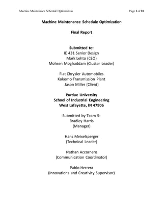
Appendix C. Machine Relabeling Sample
Above is
the
layout
diagram
for sub-
department9450 – Block Cubing– Phase 1. The redannotationsare addedtodemonstrate the
machininglabelingkey.Asseen,all machinesinthisdepartmentbeginwiththe prefix M50A (fordept.
9450, phase 1).Each spine isthenlabeledbyOP#(1A forfirstspine of OP10; 3B for secondspine of
OP30). The final letterdenotesthe specificmachine inthe spine(A,B,C,etc.if itisan NTC machine,and
r,R if it isa material-handlingmachine).Thisrelabelingwill allow ustoquicklyandeasilyidentify
machinesaccordingtothe connectionswithothersandallow ustobetterschedule withthe robot-NTC
relationof machine downtime inmind.
M50A- #X- XX
1A 3B
A
C
B
A
R
B
r
R
r
Example Shown of Machine Naming f or 9 Machines
Circled in Depart ment 9450 - Block
M50A- 1A- A
M50A- 1A- B
M50A- 1A- C
M50A- 1A- r
M50A- 1A- R
M50A- 3B- A
M50A- 3B- B
M50A- 3B- r
M50A- 3B- R
Figure 4 - Dept. 9450 Layout Diagram with Partial Machine Labeling Key
16. Machine Maintenance Schedule Optimization Page 16 of 20
Appendix D. Current Schedule Downtime Calculations
Figure 5 - Excerpt From Original Chrysler Schedule
Figure 6 - Excerpt From Name Modified Schedule
Week of September 1st
Monday 1 Tuesday 2 Wednesday 3 Thursday 4 Friday 5
AAA354818 T/M 1.00 11645 I AAA354819 T/M 1.00 11645 I AAA353598 T/M 1.00 11645 I AAA353602 T/M 1.00 11645 I AAA353597 T/M 1.00 11645 I
AAA354818 T/M 0.50 11676 I AAA354819 T/M 0.50 11676 I AAA353598 T/M 0.50 11676 I AAA353602 T/M 0.50 11676 I AAA353597 T/M 0.50 11676 I
AAA354818 T/M 0.50 11677 I AAA354819 T/M 0.50 11677 I AAA353598 T/M 0.50 11677 I AAA353602 T/M 0.50 11677 I AAA353597 T/M 0.50 11677 I
AAA354818 M/R 1.00 11633 A AAA354819 M/R 1.00 11633 A AAA353598 M/R 1.00 11633 A AAA353602 M/R 1.00 11633 A AAA353597 M/R 1.00 11633 A
AAA354818 M/R 0.66 11634 A AAA354819 M/R 0.66 11634 A AAA353598 M/R 0.66 11634 A AAA353602 M/R 0.66 11634 A AAA353597 M/R 0.66 11634 A
AAA354818 M/R 0.58 11635 A AAA354819 M/R 0.58 11635 A AAA353598 M/R 0.58 11635 A AAA353602 M/R 0.58 11635 A AAA353597 M/R 0.58 11635 A
AAA354818 M/R 0.75 11637 A AAA354819 M/R 0.75 11637 A AAA353598 M/R 0.75 11637 A AAA353602 M/R 0.75 11637 A AAA353597 M/R 0.75 11637 A
AAA354818 M/R 0.83 11638 A AAA354819 M/R 0.83 11638 A AAA353598 M/R 0.83 11638 A AAA353602 M/R 0.83 11638 A AAA353597 M/R 0.83 11638 A
AAA354818 M/R 0.50 11639 A AAA354819 M/R 0.50 11639 A AAA353598 M/R 0.50 11639 A AAA353602 M/R 0.50 11639 A AAA353597 M/R 0.50 11639 A
AAA354818 M/R 0.33 11640 A AAA354819 M/R 0.33 11640 A AAA353598 M/R 0.33 11640 A AAA353602 M/R 0.33 11640 A AAA353597 M/R 0.33 11640 A
AAA354818 M/R 0.33 11641 A AAA354819 M/R 0.33 11641 A AAA353598 M/R 0.33 11641 A AAA353602 M/R 0.33 11641 A AAA353597 M/R 0.33 11641 A
AAA354818 M/R 0.00 11643 I AAA354819 M/R 0.00 11643 I AAA353598 M/R 0.66 11643 I AAA353602 M/R 0.66 11643 I AAA353597 M/R 0.66 11643 I
AAA354818 M/R 1.00 11644 I AAA354819 M/R 1.00 11644 I AAA353598 M/R 1.00 11644 I AAA353602 M/R 1.00 11644 I AAA353597 M/R 1.00 11644 I
AAA354818 M/R 0.50 11721 A AAA354819 M/R 0.50 11721 A AAA353598 M/R 0.50 11721 A AAA353602 M/R 0.50 11721 A AAA353597 M/R 0.50 11721 A
AAA354818 Elect 0.50 538 I AAA354819 Elect 0.50 538 I AAA353598 Elect 0.50 538 I AAA353602 Elect 0.50 538 I AAA353597 Elect 0.50 538 I
AAA354818 Elect 0.16 539 I AAA354819 Elect 0.16 539 I AAA353598 Elect 0.16 539 I AAA353602 Elect 0.16 539 I AAA353597 Elect 0.16 539 I
AAA354818 M/W 0.16 4636 I AAA354819 M/W 0.16 4636 I AAA353598 M/W 0.16 4636 I AAA353602 M/W 0.16 4636 I AAA353597 M/W 0.16 4636 I
AAA354818 M/W 1.00 12134 I AAA354819 M/W 1.00 12134 I AAA353598 M/W 1.00 12134 I AAA353602 M/W 1.00 12134 I AAA353597 M/W 1.00 12134 I
AAA354818 M/W 0.25 12135 I AAA354819 M/W 0.25 12135 I AAA353598 M/W 0.25 12135 I AAA353602 M/W 0.25 12135 I AAA353597 M/W 0.25 12135 I
AAA354818 Pftr 0.25 11722 A AAA354819 Pftr 0.25 11722 A AAA353598 Pftr 0.25 11722 A AAA353602 Pftr 0.25 11722 A AAA353597 Pftr 0.25 11722 A
AAA354818 Pftr 0.25 11723 I AAA354819 Pftr 0.25 11723 I AAA353598 Pftr 0.25 11723 I AAA353602 Pftr 0.25 11723 I AAA353597 Pftr 0.25 11723 I
AAA354818 Pftr 0.50 11724 A AAA354819 Pftr 0.50 11724 A AAA353598 Pftr 0.50 11724 A AAA353602 Pftr 0.50 11724 A AAA353597 Pftr 0.50 11724 A
AAA354818 Pftr 0.50 12158 I AAA354819 Pftr 0.50 12158 I AAA353598 Pftr 0.50 12158 I AAA353602 Pftr 0.50 12158 I AAA353597 Pftr 0.50 12158 I
AAA354818 Pftr 0.75 12159 I AAA354819 Pftr 0.75 12159 I AAA353598 Pftr 0.75 12159 I AAA353602 Pftr 0.75 12159 I AAA353597 Pftr 0.75 12159 I
AAA354818 Pftr 1.00 12160 I AAA354819 Pftr 1.00 12160 I AAA353598 Pftr 1.00 12160 I AAA353602 Pftr 1.00 12160 I AAA353597 Pftr 1.00 12160 I
AAA354818 Pftr 1.00 12161 I AAA354819 Pftr 1.00 12161 I AAA353598 Pftr 1.00 12161 I AAA353602 Pftr 1.00 12161 I AAA353597 Pftr 1.00 12161 I
AAA354818 Pftr 0.50 12162 I AAA354819 Pftr 0.50 12162 I AAA353598 Pftr 0.50 12162 I AAA353602 Pftr 0.50 12162 I AAA353597 Pftr 0.50 12162 I
AAA354818 Pftr 0.08 12168 I AAA354819 Pftr 0.08 12168 I AAA353598 Pftr 0.08 12168 I AAA353602 Pftr 0.08 12168 I AAA353597 Pftr 0.08 12168 I
AAA354818 Vibr 0.08 11647 I AAA354819 Vibr 0.08 11647 I AAA353598 Vibr 0.08 11647 I AAA353602 Vibr 0.08 11647 I AAA353597 Vibr 0.08 11647 I
Week of September 1st
Monday 1 Tuesday 2 Wednesday 3 Thursday 4 Friday 5
M30B-4A-A T/M 1.00 11645 I M30B-4A-B T/M 1.00 11645 I M40A-1A-A T/M 1.00 11645 I M40A-1A-B T/M 1.00 11645 I M40A-1A-C T/M 1.00 11645 I
M30B-4A-A T/M 0.50 11676 I M30B-4A-B T/M 0.50 11676 I M40A-1A-A T/M 0.50 11676 I M40A-1A-B T/M 0.50 11676 I M40A-1A-C T/M 0.50 11676 I
M30B-4A-A T/M 0.50 11677 I M30B-4A-B T/M 0.50 11677 I M40A-1A-A T/M 0.50 11677 I M40A-1A-B T/M 0.50 11677 I M40A-1A-C T/M 0.50 11677 I
M30B-4A-A M/R 1.00 11633 A M30B-4A-B M/R 1.00 11633 A M40A-1A-A M/R 1.00 11633 A M40A-1A-B M/R 1.00 11633 A M40A-1A-C M/R 1.00 11633 A
M30B-4A-A M/R 0.66 11634 A M30B-4A-B M/R 0.66 11634 A M40A-1A-A M/R 0.66 11634 A M40A-1A-B M/R 0.66 11634 A M40A-1A-C M/R 0.66 11634 A
M30B-4A-A M/R 0.58 11635 A M30B-4A-B M/R 0.58 11635 A M40A-1A-A M/R 0.58 11635 A M40A-1A-B M/R 0.58 11635 A M40A-1A-C M/R 0.58 11635 A
M30B-4A-A M/R 0.75 11637 A M30B-4A-B M/R 0.75 11637 A M40A-1A-A M/R 0.75 11637 A M40A-1A-B M/R 0.75 11637 A M40A-1A-C M/R 0.75 11637 A
M30B-4A-A M/R 0.83 11638 A M30B-4A-B M/R 0.83 11638 A M40A-1A-A M/R 0.83 11638 A M40A-1A-B M/R 0.83 11638 A M40A-1A-C M/R 0.83 11638 A
M30B-4A-A M/R 0.50 11639 A M30B-4A-B M/R 0.50 11639 A M40A-1A-A M/R 0.50 11639 A M40A-1A-B M/R 0.50 11639 A M40A-1A-C M/R 0.50 11639 A
M30B-4A-A M/R 0.33 11640 A M30B-4A-B M/R 0.33 11640 A M40A-1A-A M/R 0.33 11640 A M40A-1A-B M/R 0.33 11640 A M40A-1A-C M/R 0.33 11640 A
M30B-4A-A M/R 0.33 11641 A M30B-4A-B M/R 0.33 11641 A M40A-1A-A M/R 0.33 11641 A M40A-1A-B M/R 0.33 11641 A M40A-1A-C M/R 0.33 11641 A
M30B-4A-A M/R 0.00 11643 I M30B-4A-B M/R 0.00 11643 I M40A-1A-A M/R 0.66 11643 I M40A-1A-B M/R 0.66 11643 I M40A-1A-C M/R 0.66 11643 I
M30B-4A-A M/R 1.00 11644 I M30B-4A-B M/R 1.00 11644 I M40A-1A-A M/R 1.00 11644 I M40A-1A-B M/R 1.00 11644 I M40A-1A-C M/R 1.00 11644 I
M30B-4A-A M/R 0.50 11721 A M30B-4A-B M/R 0.50 11721 A M40A-1A-A M/R 0.50 11721 A M40A-1A-B M/R 0.50 11721 A M40A-1A-C M/R 0.50 11721 A
M30B-4A-A Elect 0.50 538 I M30B-4A-B Elect 0.50 538 I M40A-1A-A Elect 0.50 538 I M40A-1A-B Elect 0.50 538 I M40A-1A-C Elect 0.50 538 I
M30B-4A-A Elect 0.16 539 I M30B-4A-B Elect 0.16 539 I M40A-1A-A Elect 0.16 539 I M40A-1A-B Elect 0.16 539 I M40A-1A-C Elect 0.16 539 I
M30B-4A-A M/W 0.16 4636 I M30B-4A-B M/W 0.16 4636 I M40A-1A-A M/W 0.16 4636 I M40A-1A-B M/W 0.16 4636 I M40A-1A-C M/W 0.16 4636 I
M30B-4A-A M/W 1.00 12134 I M30B-4A-B M/W 1.00 12134 I M40A-1A-A M/W 1.00 12134 I M40A-1A-B M/W 1.00 12134 I M40A-1A-C M/W 1.00 12134 I
M30B-4A-A M/W 0.25 12135 I M30B-4A-B M/W 0.25 12135 I M40A-1A-A M/W 0.25 12135 I M40A-1A-B M/W 0.25 12135 I M40A-1A-C M/W 0.25 12135 I
M30B-4A-A Pftr 0.25 11722 A M30B-4A-B Pftr 0.25 11722 A M40A-1A-A Pftr 0.25 11722 A M40A-1A-B Pftr 0.25 11722 A M40A-1A-C Pftr 0.25 11722 A
M30B-4A-A Pftr 0.25 11723 I M30B-4A-B Pftr 0.25 11723 I M40A-1A-A Pftr 0.25 11723 I M40A-1A-B Pftr 0.25 11723 I M40A-1A-C Pftr 0.25 11723 I
M30B-4A-A Pftr 0.50 11724 A M30B-4A-B Pftr 0.50 11724 A M40A-1A-A Pftr 0.50 11724 A M40A-1A-B Pftr 0.50 11724 A M40A-1A-C Pftr 0.50 11724 A
M30B-4A-A Pftr 0.50 12158 I M30B-4A-B Pftr 0.50 12158 I M40A-1A-A Pftr 0.50 12158 I M40A-1A-B Pftr 0.50 12158 I M40A-1A-C Pftr 0.50 12158 I
M30B-4A-A Pftr 0.75 12159 I M30B-4A-B Pftr 0.75 12159 I M40A-1A-A Pftr 0.75 12159 I M40A-1A-B Pftr 0.75 12159 I M40A-1A-C Pftr 0.75 12159 I
M30B-4A-A Pftr 1.00 12160 I M30B-4A-B Pftr 1.00 12160 I M40A-1A-A Pftr 1.00 12160 I M40A-1A-B Pftr 1.00 12160 I M40A-1A-C Pftr 1.00 12160 I
M30B-4A-A Pftr 1.00 12161 I M30B-4A-B Pftr 1.00 12161 I M40A-1A-A Pftr 1.00 12161 I M40A-1A-B Pftr 1.00 12161 I M40A-1A-C Pftr 1.00 12161 I
M30B-4A-A Pftr 0.50 12162 I M30B-4A-B Pftr 0.50 12162 I M40A-1A-A Pftr 0.50 12162 I M40A-1A-B Pftr 0.50 12162 I M40A-1A-C Pftr 0.50 12162 I
M30B-4A-A Pftr 0.08 12168 I M30B-4A-B Pftr 0.08 12168 I M40A-1A-A Pftr 0.08 12168 I M40A-1A-B Pftr 0.08 12168 I M40A-1A-C Pftr 0.08 12168 I
M30B-4A-A Vibr 0.08 11647 I M30B-4A-B Vibr 0.08 11647 I M40A-1A-A Vibr 0.08 11647 I M40A-1A-B Vibr 0.08 11647 I M40A-1A-C Vibr 0.08 11647 I
19. Machine Maintenance Schedule Optimization Page 19 of 20
As seeninthe figuresabove,a multi-stepprocedure wasusedtocalculate andrepresentthe
currentsystem’sdowntimeasa reference pointforournew schedulingconcept. Figure5showsa small
excerptof the file thatwe have showingthe currentschedule.First,we convertedthattohave the new
meaningful machinesnames(asshowninAppendix C) toarrive towhat isseeninFigure 6. Fromthere,
we wouldfilteroutthe unique machinesworkedonineachday, sumthe hours andinsertthe time
workedoneach intothe table seeninFigure 7.Finally,thattable hastwocolumnsforeach day: one
representinghoursworkeddirectlyonmachine andone representinghoursworkedonaconnected
material-handlingmachine (indirectdowntime).These valueswere summedacrosseachdayto getto a
final monthlyvalue foreachmachine.Finally,Figure 8showsthe sumof each month’stable givinga
total hourlydowntime foreachmachine throughoutthe full yearlyservice schedule.