Fulltext 5 baddeley

Ann. Inst. Statist. Math.
Vol. 47, No. 4, 601-619 (1995)

AREA-INTERACTION POINT PROCESSES
A. J. BADDELEY ~ AND M. N, M. VAN LIESHOUT 2

1Department of Mathematics, University of Western Australia,
Nedlands WA 6009, Australia and
Department of Mathematics and Computer Science, University of Leiden, The Netherlands
2 Department of Statistics, University of Warwick, Coventry CV4 7AL, U.K.

(Received December 6, 1993; revised January 30, 1995)

A b s t r a c t . We introduce a new Markov point process that exhibits a range
of clustered, random, and ordered patterns according to the value of a scalar
parameter. In contrast to pairwise interaction processes, this model has inter-
action terms of all orders. The likelihood is closely related to the empty space
function F, paralleling the relation between the Strauss process and Ripley's
K-fnnction. We show that, in complete analogy with pairwise interaction pro-
cesses, the pseudolikelihood equations for this model are a special case of the
Takacs-Fiksel method, and our model is the limit of a sequence of auto-logistic
lattice processes.

Key words and phrases: Clustering, empty space statistic, Hough transform,
inhibition, K-function, lattice process limits, Markov point processes, nearest
neighbour distance distribution, pairwise interaction, penetrable sphere model,
pseudolikelihood, spatial statistics, spherical contact distance distribution, sta-
tionary point process, Strauss model, Takacs-Fiksel method.

i. Introduction

Since the introduction of Markov point processes in spatial statistics (Kelly
and Ripley (1976), Ripley and Kelly (1977)) (the very similar concept of a Gibbs
point process was already known in statistical physics (Ruelle (1969), Chapter 3,
P r e s t o n (1976))) a t t e n t i o n has focused on the special case of pai~vise interac-
tion models. These provide "a large variety of complex p a t t e r n s starting from
simple potential functions which are easily interpretable as attractive a n d / o r re-
pulsive forces acting among points" (Mase (1990)). A great deal is u n d e r s t o o d
a b o u t pairwise interaction models because they are very natural with respect to
the derivation of conditional probabilities, Papangelou conditional intensities and
Palm distributions; they are simple exponential families whose sufficient statis-
tics are often related to the popular K-function; and they are very amenable to
simulation and iterative statistical methods.
However, pairwise interaction processes do not seem to be able to produce
clustered p a t t e r n s in sufficient variety. T h e original clustering model of Strauss

601

602 A. J. B A D D E L E Y AND M. N. M. VAN L I E S H O U T

(1975) turned out (Kelly and Ripley (1976)) to be non-integrable for parameter
values ~, > 1 corresponding to the desired clustering; Gates and Westcott (1986)
showed that partly-attractive potentials may violate a stability condition, implying
that they produce extremely clustered patterns with high probability; and recent
sinmlation experiments by Moller (1994) suggest that the behaviour of the Strauss
model with fixed 77 undergoes an abrupt transition from "Poisson-like" patterns
to tightly clustered patterns rather than exhibiting intermediate, moderately clus-
tered patterns.
In this paper we introduce a family of Markov point processes that yield both
moderately clustered and moderately ordered patterns. They can be described as
having interactions of infinite order. In the simplest case the probability density
of a point pattern x = {Xl . . . . . :r,,} (7~ _> 0) in a window A C_ ~2 is defined to be

(1.1) p ( x ) = 03"') '-''l~)

where .u(a:) is the area of the plane set formed by taking the union of discs of
radius r centred at the points xi. Here 13.7. r > 0 are parameters and c~ is the
normalising constant. Compare this with the pairwise-interaction Strauss process
in the same situation,

(1.2) p(m) = a / Y ' 7 "~{~')

where s(x) is the number of pairs of distinct points :ri, xj that lie within a distance
r' of one another. Both densities reduce to a Poisson process when 7 = 1, and
exhibit ordered patterns for 0 < ") < 1. Our process (1.1) is well-defined for all
values of ")' > 0 and produces clustering when ~ > 1. The clustered case "y > 1
of (1.1) is identical to tile 'penetrable sphere model' of liquid-vapour equilibrium
proposed by Widom and Rowlinson (1970), see also Hammersley et al. (1975) or
Rowlinson (1980, 1990). Our Definition 1 embraces both clustered and ordered
types and Definition 2 below is a further generalisation to non-spherical shapes
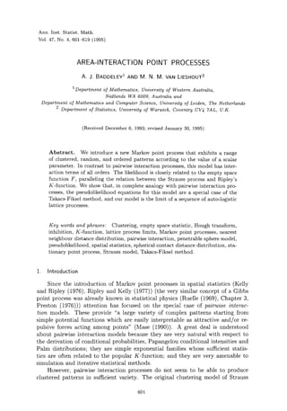
and non-uniform measures. Figure 1 shows simulated realisations of (1.1).
It is useful to note that computation of .u(z) is easy in an image processing
context, using the distance transform algorithm (Rosenfeld and Pfalz (1968)).
The plan of the paper is as tbllows. In Section 2 we define the process and check
that it is integrable for all parameter values. We show that it is a Markov point
process with interactions of infinite order, and give various physical interpretations.
In Section 3 we prove that the process satisfes a stability condition and that there
is a corresponding stationary Gibbs process on ~t. Section 4 briefly discusses
simulation techniques.
In Section 5 we consider statistical inference. First we show that (1.1) is
connected to the popular empty space statistic F in the same way"that the Strauss
process (1.2) is related to 1Ripley's K-flmction. We show that pseudolikelihood
inference for the area-interaction process is a special ca,se of the Takacs-Fiksel
method, analogous to the situation for pairwise interaction processes (Diggle et
al. (1994), SSrkk'a (1989), Ripley (1989)). Finally in Section 6 we prove that the
area-interaction process is the linfit (weakly and in total variation) of a sequence
of autologistic lattice processes, extending the limit theorem of Besag et al. (1982).

AREA-INTERACTION POINT PROCESSES 603

+ + +§ + +
+ §
+ +
+
+ + + § +.*
+ +
+
+ + + *
§ + + +
§ + +
§ §
+ § + § § + + § §
§ § § + + + , +
+

+ + + + +
4+
+
+
+ +
§ ++
g
+ + * +
§
§
* +
+
+** +
+ § +F§ + + +
+ + ++ +
+ +
§ + + + +
§ g +
§ § § + + +
§247
§ + + 9+ +
+ + + §
++ + +
§
+ § ++ §
+ §
+
+ + g § §
+
+ ++ +
9 + +
+ § + + + +
+ +
f + + ,~ § + .
§ §
+ + + +
+ + + +
o
I I I ---r-- I

50 100 150 200 250 0 50 100 150 200 250

Pig. 1. S i n m l a t e d r e a l i s a t i o n s of an a r e a - i n t e r a c t i o n p r o c e s s c o n d i t i o n a l on n = 1 0 0
p o i n t s , w i t h r = 5 in a w i n d o w of size 2 5 6 x 2 5 6 . Left: o r d e r e d p a t t e r n , 7 = 0 . 9 7 1 1 ,
~-25~ = 10; Righ.t: c l u s t e r e d p a t t e r n , 7 = 1 . 0 2 9 7 5 , 7 -257r = 0 . 1 .

2. Definition of process

2.1 Preliminaries
As usual for Gibbs point processes we treat separately the cases of a finite
point process (say, points in a bounded region A c_ [R~) and a stationary point
process on IRd.
The formal construction of finite Gibbs point processes is described in Daley
and Vere-Jones ((1988), p, 121 if), Preston (1976) or e.g. Section 2 in Baddeley
and Moller (1989). Briefly, let X be a locally compact complete separable metric
space (typically [Rd or a compact subset). A realisation of a finite point process is
a finite set of points

X = {2:1 . . . . . :/2,,}, X i E ,~", 'n ~ 0 .

The space of all possible realisations shall be identified with the space Rf of all
integer-valued measures on X w h i c h h a v e finite total mass and are simple (do not
h a v e atoms of mass exceeding 1). Write n(a:) for the total mass (=total n u m b e r
of points), and mB for x restricted to B C_ X. The a-algebra H a` on !Rf is the
Borel or-algebra of the weak topology, i.e. N " / i s the smallest a-algebra with respect
to which the evaluation m ~ n(a:B) is measurable for every (bounded) Borel set
Bc_X.
Given a totally finite, non-atomic measure p on X, construct the Poisson
process of intensity # (typically p is the restriction of Lebesgue measure to a
compact window A C_ ~d, yielding the unit rate Poisson process restricted to A).
Let re be its probability distribution on (Rf,A/'I). Then we construct (Gibbs) point
processes by speci ,fying their density with respect to 7r. A density is a measurable
function p : Rf ---+ [0, oe) that is integrable with respect to re.

604 A.J. BADDELEY AND M. N. M. VAN L I E S H O U T

T h e general pairwise interaction process on a compact region A C_ ~ d is then
defined by its density
p(~) = a 1-I b(.~,~) I I ~(x~, xj)
i i<j

(with respect to the unit-rate Poisson process on A) where b, c are nonnegative
measurable functions and a is the normalising constant. T h e Strauss process (1.2)
is the special case where b(.) - ~ and c(u, v) = 7 if 0 < Ilu -~'ll -< ~, c(,~,, ,,) = 1
otherwise. Kelly and Ripley (1976) pointed out that. (1.2) is not integrable for
7>1.

2.2 Area-interaction process

DEFINITION 1. ( S t a n d a r d case) T h e area-interaction process in a c o m p a c t
region A C_ ~d is the process with density

(2.1) p(x) = a~,3"(~)')'-'''(U'-(~))

with respect to the unit rate Poisson process on A, where/3, 7, r > 0 are p a r a m e t e r s
and ct is the normalising constant, 'm is Lebesgue measm'e, and

g,.(x) = 0 B(:r~, r)
i=l

is the union of spheres or discs of radius r centred at the points of the realisation,
B(:~~,,) -- {a e ~d: Ila --:~',11 --< "}"

For ~ = 1 this of course reduces to a. Poisson process with intensity/3p. It is
intuitively clear that for 0 < y < 1 the p a t t e r n will tend to be 'ordered' and for
7 > 1 'clustered' (we make this precise in Subsections 5.1 and 5.3). T h e clustered
case was introduced by W i d o m and Rowlinson (1970). See also H a m m e r s l e y et al.
(1975) or Rowlinson (1980, 1990).
Various modifications are of interest, for example, one may wish to replace
U,.(x) by A A U~(x), or to allow the radii of the discs B ( x i , r ) to vary across the
region (Lawson (1993)). More generally, the discs B ( x i , r ) can be replaced by
compact sets Z(xi) depending on xi. We assume t h a t the mapping Z onto the
space K] of all compact subsets is continuous with respect, to the myopic topology
( M a t h e r o n (1975), p. 12) generated by { K E ~2 : K n F = ~} for all closed F C X
and { K E/C : K N G r 0} for all open subsets G C_ X.

DEFINITION 2. (General case) Let lJ be a totally finite, Borel regular mea-
sure on 2( and Z : 2( ~ K: a myopically continuous function, assigning to each
point a E X a compact set Z(a) C_ 2(. T h e n the general area-interaction process
is defined to have density

(2.2) p(m) = a/3~(x)7-~(u(~))


with respect to rr (the distribution of the finite Poisson process with intensity #),
where U ( x ) is the compact set [,Ji~__lZ ( x i ) .

In a parametric statistical model the measure u and the definition of Z(.)
might also be allowed to depend on the parameter 0.

LEMMA 2.1. The density (2.2) is measurable and integrable for all fixed val-
ues of [3, 3" > O.

PROOF. Let t > 0 and consider V = {x E ~}~f : b'(U(x)) < t}. We show t h a t
V is open in the weak topology.
Choose x E V. Since u is regular, there is an open set G c_ X containing U ( x )
such t h a t u(G) < t. Consider W = {y E )Rf : U ( y ) C_ G}; we have y E reV iff y has
no points in H = {a E 32 : Z ( a ) A G ~ r 0}. Now H is closed in 32 since a ~-+ Z(a) is
myopically continuous and the class of all compact sets intersecting a given closed
set is closed in the myopic topology on/C. Thus W = {y E ~S : n ( y H ) = 0} is
open in the weak topology. But x E W C_ V and x was arbitrary so V is open in
the weak topology.
In fact this shows t h a t x ~ u ( U ( x ) ) is weakly upper semicontinuous. It
follows t h a t the map g : .~f -+ [0, oc) defined by x ~ e x p [ - u ( U ( x ) ) log 3`] is weakly
upper semicontinuous for 7 E (0, 1) and lower semicontinuous for 3' > 1. Hence g
is measurable. By definition of the weak topology, x ~-+ [3'~(~) is measurable, and
hence the density (2.2) is met~surable.
To check integrability, observe t h a t

(2.3) o <_ < <

Now the fimction f ( x ) = fl~'(~) is integrable, yielding the Poisson process with
intensity measure fl#. Hence (2.2) is dominated by an integrable function, hence
integrable. []

In fact (2.3) establishes a slightly stronger result.

LEMMA 2.2. The distribution P~,~ of th,e general area interaction process
is uniformly absolutely continuous with respect to the distribution of the Poisson
process 7r/3 with intensity fl#, that is its Radon-Nikodym derivative is uniformly
bounded in x.

In particular, the general area-interaction model satisfies the linear stability
condition in Gates and Westcott (1986). Explicit bounds on the density f with
respect to a Poisson process with intensity [3tt are

m i n { 3 ' , ( x ) .,/-,,(x)} G f <_ max{~ "(x), 3"-~(x)}.

This suggests t h a t the 'singularity' (highly clustered behavior) of the Strauss model
is unlikely for moderate values of 3'.


As usual, the normalising constant ct is difficult to compute, since
ct -1 = E[y~(x),,/-~(u(x))

where the expectation is with respect to the reference Poisson process; this entails
computing the moment generating function of ~(U(X)), or equivalently, the va-
cancy distribution in the coverage problem (Hall (1988)). A notable exception is
the 1-dimensional penetrable sphere model of Widom and Rowlinson (1970).

2.3 M a r k o v property
The purpose of this paragraph is to place (2.2) in the context of Markov point
processes in the sense of Ripley and Kelly (1977), see (Baddeley and Moller (1989),
Kendall (1990)) 9 Their defining property is that the likelihood ratio p(~u{~}) for
p(x)

adding a new point a to a configuration x depends only on those x.i E x that are
'close' to a. Surveys can be found in Cressie ((1991), pp. 673-689), Stoyan et al.
((1987), pp. 148-166) and Stoyan and Stoyan ((1992), pp. 342-359).
As in Baddeley and Van Lieshout (1991, 1992, 1993) define two points a, b E X
to be neighbours (and write a ~ b) whenever Z ( a ) N Z(b) ~ ~. In the standard
case a ~ b iff I l a - bll < 2r.

LEMMA 2.3. The area-interaction p w c e s s (2.2) is a M a r k o v point process
with. respect to ~ in the sense of Ripley and Kelly (1977).

PROOF. The likelihood ratio
(2.4) p(= u {a}) _ 9 _,~(z(o)u~)~
p(=)
is computable in terms of a and {xi : x / ~ a}, since

Z(a) u ( ~ ) -- Z(a) n Z(~,)

= z(a) n (.~)
X

Hence (2.2) defines a Markov point process with respect to ~. []

The Ripley-Kelly analogue of the Hammersley-Clifford theorem (Ripley and
Kelly (1977)) then implies that the density p can be written as a product of clique
interaction terms
J'(~) = 1-I q(Y)
yc_~
where q ( y ) : 1 unless yi ~ yj for all elements of y. To compute the interaction
terms explicitly, invoke the inclusion-exclusion formula:

.(u(x)) = ~ . ( z ( z i ) )
i=1

i<j i=l


which gives

q(0) =

(2.5)
q({a}) = /~,~-v(Z(a))
q( {Yl, . . . , Yk } ) : "~ (-1)ku(N:'=lZ(yi)) k>2.

T h a t is, the process exhibits interactions of infinite order.
It is also trivial to verify t h a t the process satisfies a spatial Markov p r o p e r t y
(cf. Kendall (1990), Ripley and Kelly (1977)). Define the dilation of a set E _C X
by

(2.6) D z ( E ) = {u C X : 3e E E such t h a t Z(u) N Z(e) r 0};

in the s t a n d a r d case this becomes the classical dilation of m a t h e m a t i c a l morphol-
ogy

(2.7) D z ( E ) = {u 9 ~d : d ( u , E ) <_ 2r}

where d(u, E ) = inf{Hu - vii : v 9 E}. T h e n the spatial Markov p r o p e r t y states
t h a t the restriction of the process to E is conditionally independent of the restric-
tion to D z ( E ) ~ given the information in D z ( E ) E.

2.4 Limiting cases
Here we s t u d y the convergence of the area-interaction process as "y ~ 0, ~ .
Let u* = maxx u ( U ( x ) ) , typically the measure of the observation window or
its (generalised) dilation and

H = { x : u ( U ( x ) ) = u*}.

Further let 7r/3 be the distribution of the Poisson process of r a t e / 3 in A and finally,
in the s t a n d a r d case, denote

HC = {z: =

LE~VIMA 2.4. Let P/~,~ be the distribution of the area interaction process with
density (2.2).
If "~ -~ 0 with/3 fixed, then P~,~. converges to a uniform process on H, i.e.
. 3(E n
In the standard case, if "~ ---* 0 and ,2 ---* 0 so that/3"7 - ' r : ---* ~ E (0, oc), then
P~,~ converges to P ( E ) = 7r((E A H C ) / T c ( ( H C ) , a hard core process.
If ~ ---+ oo with/3 < oo fixed, then PZ,~ converges to a process that is e m p t y
with probability 1.

PROOF. First consider ~ ---* 0. T h e n fw"-~(u(~))dTrZ(x) ~ 7re(H), hence

7 "'-'(U(~)) l{x C H}
p~,~(x) = f~/.._.(u(~))dTcZ(x ) 7cZ(H)


from which the first assertion follows. To prove the second assertion, note t h a t for
m ( U ~ ( x ) ) < n ( x ) r r r 2, 3.......-~.... (u',.(~)) __+ O. Hence

r C HC}
JHc
T h e third s t a t e m e n t follows similarly, by noting t h a t the density converges point-
wise to zero unless the p a t t e r n is empty. []

2.5 Interpretation and motivation
A r e a - i n t e r a c t i o n seems a plausible model for some biological processes. For
e x a m p l e the points xi m a y represent plants or animals which c o n s m n e food within
a radius r of their current location. T h e t o t a l a r e a of accessible food is t h e n U ( x ) ,
and the herd will tend to m a x i m i s e this area, so an a r e a - i n t e r a c t i o n model with
7 < 1 is plausible. A l t e r n a t i v e l y a s s u m e t h a t the animals or plants are hunted
1)3, a p r e d a t o r which a p p e a r s at a r a n d o m position and catches any p r e y within a
distance r. T h e n U ( x ) is the area of wflnerability, and the herd as a whole should
t e n d to minimise this (see, e.g. H a m i l t o n (1971)) so an a r e a - i n t e r a c t i o n model with
~' > 1 is plausible.
T h e following trivial i n t e r p r e t a t i o n s are also possible:

LEMMA 2.5. Let X , Y be independent Poisson pTvcesses in A with intensity
measures ,'3p and ]log').lu 7rspectively. If "y > 1 then the conditional distribution of
X given { Y A U ( X ) = 0} is an area-interaction process with, parameter 7. I f 7 < 1
then the conditional distribution, of X given {Y C U ( X ) } is an area-interaction
process with parameter "y.

PROOF. If ~ > 1

P{}/" 0 U(X) = 0 ] X} ~- e - u ( U ( X ) ) l ~ ~_ , . y - u ( u ( x ) )

hence the conditional distribution of X given Y N U ( X ) = 0 has a density propor-
tional to the right h a n d side. Sinfilarly if "~ < 1

P{a g u(x) I x } = p ( y (A U(X)) = O}
= eu(AU(X))log7 = .,fu(A),)-u(U(X)). []

O t h e r i n t e r p r e t a t i o n s are available in t e r m s of spatial b i r t h - a n d - d e a t h pro-
cesses (see Section 4). Briefly, if the points represent plants again, we m a y consider
a process in which existing plants have e x p o n e n t i a l ( I ) lifetimes, and a new seed
takes root at location a with r a t e p ( x @ { a } ) / p ( x ) related to the a r e a accessible
to a t h a t is not already accessible to an existing plant. A l t e r n a t i v e l y we m a y
assume the plants or animals arrive at a c o n s t a n t r a t e uniformly over space, and
an existing a n i m a l xi dies at a rate p ( x { x i } ) / p ( x ) related to the risk of being
a t t a c k e d by a p r e d a t o r .


3. Stationary area-interaction process

Here we use the m e t h o d s of P r e s t o n (1976) to check t h a t the area interaction
model (standard case) can be considered as the restriction to a b o u n d e d sampling
window of a s t a t i o n a r y point process on the whole of ~ .
Let ~ be the space of all locally finite counting measures (i.e. integer-valued
R a d o n measures) on ~d with the vague topology, and .h/" its Borel a-algebra; t h a t
is, Af is the smallest ~-algebra making x ~-+ n ( x B ) measurable for all b o u n d e d
Borel sets B.
Write C for the class of all b o u n d e d Borel sets in Nd. For every B E C let
~B be the subspace of those x E ?R contained in B (i.e. putting no mass outside
B), JV'B C N" the induced G-algebra on ~ and rcJ~ the distribution on ( ~ , N ' ) of
B
the homogeneous Poisson process of rate /) on B. Note t h a t any x E R can be
decomposed as x = XB U XB~:. Define f B : ~ __~ [0, c~) by

(3.1) f S ( x ) = aB( XB,,)7-"(U,-(~)nB+, )

where U,.(x) = U~:,E~ B ( x i , r), Be~ the dilation of B by a ball with radius r and
O'B(XB~) is the normalising constant

' B

To check t h a t (3.1) is measurable and integrable, observe t h a t

U,,(x) n Be, = U,.(xs§ n B+,.

so t h a t the map g : x ~ m(U,.(x) N B@~) is measurable with respect to .N'Be>.
and a fortiori with respect to A/'. Clearly g is integrable with respect to rc'~
B~2,-"
Regarding the Poisson process on Be2~ as the independent superposition of Poisson
processes on B and Bo2,. B we can apply Fubini's theorem to integrate over the
B c o m p o n e n t and conclude t h a t CtB(') -1 is YB§ and integrable.
Hence, (3.1) is Af-measurable and integrable, and we may define for x E .~, F E A/"

(3.2) ~:B(X, F) = s 1F(XB~ U y),fB(xB,: O y)dTr~(y).
B

THEOREM 3.1. There exists a stationary point process X on ~d such that

P { x E F I XB~-} = ~:B(X, F) a.s.

for" all B E C and F E N'. That is, (3.2) is a specification without forbidden states
(Preston (1976), p. 12) and the distribution of X is a stationary Gibbs state 'with
this specification. The corresponding potential V : ,~f ---+0~,

v ( x ) = ( - log-y),,~(u(x))


is stable (Preston (1976), p. 96).

Note that this result does not exclude the possibility that the Gibbs state is
not unique, i.e. there may be 'phase transition' (Preston (1976), p. 46).

PROOF. First we prove consistency condition (6.10) of Preston ((1976),
p. 91). For any bounded Borel s e t s A c_ B

.fB(x) aB(XB~) -,,,(U,.(x..v-)nB§
f A ( x ) -- aA(XA,,)~/
On the other hand

s .fS(XA~ U y)drC~A(y) = aB(XB~) ~ a ~/-"(u"(~":uu)cn'*")dzc!~(Y)

Since

m(U,-(XA~ O y) N Be,. ) = m(U~(Xd~ U y) N Ae,. )
+ m(U,-(XA~) C~Be,. Ae,.),

f~..~ fB(xAc t2 y)drcl~(y ) = fS(x)/fA(x). It follows (Preston (1976), pp. 90-91)
that {tcB : B E C} is a specification in the sense of (Preston (1976), p. 12).
Now we check the conditions of Theorem 4.3 of Preston ((1976), p. 58). Con-
dition (3.6) of Preston ((1976), p. 35) is trivially satisfied. Arguments sinfilar
to those used to derive Lemma 2.2 above yield that for any K E K~ the fanfily
{Tr/~-(y, .)}y~.~ considered as a class of measures on (~,Aff<) is unifornfly abso-
lutely continuous with respect to rc~.; hence Preston's condition (3.11) (Preston
(1976), p. 41) holds, which implies his (3.10). It remains to check (3.8) of Preston
((1976), p. 35). Let K: be the class of all compact subsets of It~d; then we claim
that

for any B E C and F E A/'K where K E ]C, there exists L E ]C such that
riB(', F) is measurable with respect to AlL.

To check this, choose L to contain K t2 Be2 ,. and observe that 1F(XB; [2 y) and
fu(x~ O y) are measurable with respect to HL | then apply Fubini's theorem
(in the same way as was used to prove measurability of (3.1)). This proves the
claim, which implies Preston's (3.8) and hence the conditions of his Theorem 4.3.
It is easy to see that V is the unique canonical potential corresponding to our
densities fB (cf. Preston (1976), p. 92). Since 0 <_ m(Ur(x)) _< rcr2n(x), V is
stable. []


4. Simulation

In this section we explore methods for simulating (2.1) using spatial birth-
and-death processes (Baddeley and Moller (1989), Moller (1989), Preston (1977)).
Other techniques such a~s Metropolis-Hastings algorithms (Geyer and M011er
(1993), Moller (1992)) are clearly possible. The general cause can be dealt with
similarly, but for simplicity we focus on the standard case.
A spatial birth-and-death process (Preston (1977)) is a continuous time, pure
jump Markov process with states in ~ f specified by its transition rates D ( x
{x~},xi) for a death (transition from x to x {xi}) and b(x,u)dp(u) for a birth
(transition from x to x U {u}). Write D ( x ) = ~ : ~ . ~ D ( x {xi},x~) and B ( x ) =
fA b(x, u)dp(u) for the total transition rates out of state x.
We consider two standard cases, the constant death rate process (Ripley
(1977)) which has death rate D ( x {xi}, xi) = 1 and birth rate

u
(4.1) b(x,u) - - - / 3 e x p [ - log(7)u(U(x U {u}) U(x))]

and the constant birth rate process which has b(x, u) -- 1 and

(4.2) D ( x {xi},xi) - -/3 exp[log(7),(u( ) u(x {x,}))].

LEMMA 4.1. For any % the constant death .rate and constant birtlz rate pro-
cesses exist and converge in distribution to the area-interaction process (2.1) from
any initial state.

PROOF. Note that p(x) > 0 for all x. Hence we only have to check the
summability condition of Theorem 2.10 in Baddetey and Moller (1989) (see Propo-
sition 5.1, Theorem 7.1 in Preston (1977)). These are obviously satisfied since the
birth rates are bounded by a constant times/3 '~(~). []

On a practical note, computation of the ratios (4.1) or (4.2) at every u is
equivalent to computing the Hough transform of U(x); see e.g. Baddeley and
Van Lieshout (1992) or Illing~vorth and Kittler (1988). The fixed n, alternating
birth/death technique of Ripley (1977) was used to generate Fig. 1. This requires
that we generate a point u E A with density proportional to (4.1); this is relatively
easy using rejection sampling, since (4.1) is dominated by a known constant by
virtue of (2.3) which in practice will be a good bound when "7 is not far from 1.

5. Inference

5.1 Sufficient statistics, exponential families
Consider a family of area-interaction processes (2.1) indexed by parameter
0 -- (/3, "),), with r and A C_ ~a fixed. This is an exponential family with canonical
sufficient statistic
T(x) = M ( x , .))

612 A. J. BADDELEY AND M. N. M. VAN LIESHOUT

where

r) = = m (0 B(x ' r)) "

Modifying this slightly we obtain a connection with the 'empty space statistic'
F(t) -- P { X A B(O,t) r 0} (Diggle (1983), Ripley (1981)). Define

(5.1) F ( r ) = m(A(_~) n (Ui%l B(xi, r)))
m(A(_r))

where
A(-t) = {a r A : B(a,t) C_ A}.

This is the 'border method' (Ripley (1988), p. 25) or 'reduced sample' estimator
(Baddeley and Gill (1992)) of the empty space function.

LEMMA 5.1. (n(x), fi) is a sufficient statistic for the area-interaction process
(2.2) 'with. parameters (fi, ~/) when Z(a) = B(a, r) and the measure ~, is Lebesgue
measure restricted to A(-r).

The canonical parameter is 0 = - log ~/but we prefer to use "), to maintain the
comparison with the Strauss process.

5.2 Maximum likelihood
As usual for Markov point processes, the likelihood (2.2) is easy to compute
except for a normalising constant c~ that is not known analytically. Maximum
likelihood estimation therefore rests on numerical or Monte Carlo approximations
of c~ (Ogata and Tanemura (1981, 1984, 1989), Penttinen (1984)) or recursive ap-
proximation methods (Moyeed and Baddeley (1991)). For a more detailed review
see Diggle et al. (1994), Ripley (1988) or Geyer and Thompson (1992).
We will not explore this further here, except to note that the maximum like-
lihood estimating equations are as usual

(5.2)
(5.3) = Eg,..(u(x))
where x is the observed pattern and X is a random pattern with density (2.2).
For the model conditioned on n(x) = n the ML estimating equation is analogous
to (5.3) with fl absent.
Other estimation techniques have been proposed in Diggle et al. (1987) and
Diggle and Gratton (1984).


5.3 Takacs-Fiksel
The Takacs-Fiksel estimation method exploits the Nguyen-Zessin identity
(Nguyen and Zessin (1979))

(5.4) Afg!~f(X) = n=[A(a;X ) f ( X ) ]

holding for any bounded measurable non-negative function f : R ~ R+ and any
stationary Gibbs process X on Nd with finite intensity A, see G15tz (1980a, 1980b),
Kozlov (1976), Matthes et al. (1979), Kallenberg (1984) or Ripley ((1988), pp. 54-
55), Diggle et al. ((1994), w 2.4). The expectation on the left side of (5.4) is
with respect to the reduced Palm distribution of X at a E Rd and A(a; x) is the
Papangelou conditional intensity of X at a. The idea (Fiksel (1984, 1988), Takacs
(1983, 1986)) is then to choose suitable functions and estimate both sides in the
above formula. The resulting set of equations is solved, yielding estimates for the
parameters of the model.
When X is a Gibbs point process the conditional intensity can be computed
in terms of the potential (Kallenberg (1984)). For the standard area-interaction
process the conditional intensity is

p(~ u {~}) _/3,./-.~(B(~,r)U,.(~{~})).
(5.5) ,X(u; x) -

I n case u ~ x t h i s r e d u c e s to

/3,./-m( B(u,r) U~(~)).

One interesting instance of (5.4) is

l { x N B(0, s) = 0}
f(x) =
~(o;x)

using 0 as an arbitrary point of Nd (cf. Stoyan et al. (1987), (5.5.18), p. 159). Then
~[A(0; X ) f ( X ) ] = 1 - F(s) where F(s) = P{X N B(0, s) r 0} is the empty space
function of X. Now if s > 2r then

AE0f(X ) = A / I { X N B(0, s) = O}/3-17'~(B(~
= A / I { X n B(0, s) = O}~-lTm(B(~

: /~/3--1"}jrr~-[1 -- a(8)]

where G(s) = P0{X N B(0, s) r 0} is the nearest neighbour distance distribution
function of X. Equivalently,

1 - G(s) _ / 3 7 _ ~
(5.6) ~ 1 - F(~)


for all s > 2r. This suggests that parameter estimates for the area-interaction
process can be extracted directly from the standard statistics F and G. For further
development of this idea see Van Lieshout and Baddeley (1995).
The identity (5.6) provides a further description of the typical pattern gener-
ated by an area-interaction process, since the ratio (1 - G)/(1 - F) is less than
1 for clustered patterns, 1 for a Poisson process and greater than 1 for regular
patterns.

5.4 Pseudolikelihood estimation
The pseudolikelihood is defined (Besag (1977), Jensen and Moller (1991)) by

(5.7) PL(/3,~/; x) = exp { - ~4 ,~(u; x)du.} f i A(xi; x)
i=1

and can be interpreted as the limit case of pseudolikelihood for lattice processes
(Besag (1977), Besag et al. (1982), Jensen and Moller (1991)). For Markov pro-
cesses of finite range, maximum pseudolikelihood estimators are consistent (Jensen
and M011er (1991)); asymptotic normality is considered in Jensen (1993).
For the area-interaction model, the maxinmm pseudolikelihood estimates of/3
and 3' are the sohltions of

(5.8) n, =/3 ./~ "/-ti U)dzt
71

(5.9) t(xi) = / 3 ~2 t(u)')'-t(")d~t
i=l

where t(r -- X U,.(x X
Note that these have exactly the same form as the pseudolikelihood equations
for the Strauss model (Ripley (1988), p. 53); in that case - t ( u ) is the nmnber of
points in a: with 0 < - .,',11 -< ,.
For inhibitory pairwise interaction models it is known that pseudolikelihood
estimation is a special case of the Takacs-Fiksel method when the interaction
radius r is fixed (Diggle et al. ((1994), Section 2.4), Ripley ((1988), p. 54), S/irkk/i
((1990), Section 4)). The same is true for the area-interaction model.

THEOREM 5.1. For a stationary, area-interaction process, the pseudolikeli-
hood equations(5.8) and (5.9) are special cases of the Takacs-Fiksel method.
PROOF. Take f to be either of

f/3(x) =/3 -1,
L ( x ) = - 7 - ' m ( B ( o , , ' ) u,,(x {0})).
These are the partial derivatives of log A(0; x) with respect to /3 and % When
f = f~ an unbiased estimator for the left hand side of (5.4) is
n 1
m.(A)/3


and, by stationarity,
1
m(A) fA ~[3"/-t('')du
is an unbiased estimator of the right hand side. W h e n f = fT, the average over
the observed events
n 1 @, --t(xi)
re(A) n/--."i=1 ?'
is an unbiased estimator of the left hand side of (5.4) by the Campbei1-Mecke
formula, while an unbiased estimator for the right hand side is the window mean

)aa.
Y

These reduce to (5.8)-(5.9). []

6. Approximation by lattice processes

Besag et al. (1982) proved t h a t any purely inhibitory (or hard core) pairwise
interaction point process is the weak limit of a sequence of lattice processes, and
remark t h a t this is also true of general Gibbs point processes, again of purely
inhibitory type. Here we prove a similar result for the area-interaction model,
which is not purely inhibitory.
Consider a partition { C 1 , . . . , C,,} of the observation window A and choose
fixed points ~i C Ci. Denote the area of Ci by Ai > 0 and the set of all repre-
c
sentatives by E. We shall construct a 0, 1-valued stochastic process n = {hi : i =
1 . . . . , m} which is auto-logistic,

P(n = 1 I',j, J r i)
(6.1) P(nz = 0 I r "i) = tt (C )

where
pi(Ci) = Ai U q((i U y),l(y);
the p r o d u c t ranges over all (possibly empty) subsets of E {~i}, the set function q
is the clique interaction function (2.5) of the area-interaction model, and 71(y) =
[I~j~y 'nj is either 0 or 1, defining 0 ~ = 1.
Given a realisation of n, construct a point process x such t h a t if ni = 0
then x N Ci is empty, while if ni = 1 then x ~ Ci consists of one point uniformly
distributed in Ci independently of other points.

LEIVIMA 6.1. The conditional distributions (6.1) specify a distribution fo'r n
of the forth
P ( n ) _ ]-[ A!~, H q(y),l(y).
.l.J. t
i O:~yC_Z


The point process x is absolutely continuous with respect to the unit rate Poisson
process on A, with, density

f(x)=f(~) H q(Y)"=(u)"
O#yC =

Here '7=(Y) = 1-In( x A Cj) and the product ranges over all j such th,at (j E y.

PROOF. Use Besag's factorisation theorem (Besag (1974), p. 195). []

THEOREM 6.1. Consider a sequence of partitions C~ = {C,-.1 . . . . . C,.,,,(,.)}
such that maxi diam(Cr,i) --+ O. Then the corresponding point process x (~) co'n-
verges weakly and in total variation to the area-interaction process.

PROOF. Let fr be the density of x ('). For fixed x

f (x)
q(y) : / 3 . ( ~ ) 7 - , . ( u ( ~ ) )
r162

since all ceils contain at most one point, and q is continuous in all its arguments.
By dominated convergence,

- --aTrtx )~ = -;
f,.(O) f,.(O) c~ a

thus,
f,,(x)
L.(x) - --L.(O) -+ p ( x )
f,.(•)
pointwise and the theorem is proved. []

7. Final remarks

The Strauss process is a special case of the general pairwise interaction process.
In the same way, there is a generalisation of the area-interaction process to a
process with density

where d ( x , u) = mini Hxi - "ull and f : [0, ~c] + ( - o c , oc]. The area-interaction
process is then the special case f ( t ) = l[t _< 7"]. Thus f is the analogue of the
general interaction function in pairwise interaction.


Acknowledgements

This research was carried out at CWI (both authors) and the Free University
of Amsterdam (Van Lieshout). We thank Profs. Besag, Moiler and Oosterhoff
for helpful COlllinents and Prof. Ogata and an anonynlotls referee for drawing our
attention to the penetrable sphere model.

REFERENCES

Baddeley, A. J. and Gill, R. D. (1992). Kaplan-Meier estimators for interpoint distance distri-
butions of spatial point processes, Research Report, 718, Mathematical Institute, University
of Utrecht. The Netherlands.
Baddeley, A. J. and Moiler, ,]. (1989). Nearest-neighbour Markov point processes and randonl
sets, Internat. Statist. Rev., 57, 89-121.
Baddeley, A. J. and Van Lieshout, hi. N. M. (1991). Recognition of overlapping objects using
Markov spatial models, Tech. Report, BS-Rgl09, CWI, Amsterdam.
Baddeley, A. J. and Van Lieshout, M. N. M. (1992). ICM for object recognition, Computatiorml
Statistics (eds. Y. Dodge and J. Whittaker), Vol. 2, 271-286, Physics/Springer, Heidelberg.
I3addeley, A. ,1. and Van Lieshout, M. N. hi. (1993). Stochastic geometry models in high-level
vision, Statistics and Images (eds. K. Mardia and G. K. Is:anti), Vol. 1, ,]ouT"nal of Applied
Statistics, 20, 233 258, Carfax, Abingdon.
Besag, J. (1974). Spatial interaction and the statistical analysis of lattice systems (with discus-
sion), J. Roy. Statist. Soc. Set. B, 36, 192-236.
Besag, J. (1977). Sonm methods of statistical analysis for spatial data, }3ull. Internal. Statist.
lrlst., 47, 77 92.
Besag, J., Milne, R. and Zachary, S. (1982). Point process limits of lattice processes, J. Appl.
Probab., 19, 210-216.
Cressie, N. A. C. (1991}. Statistics for Spatial Data, Wiley, New York.
Daley, D. ,1. and Vere-Jones, D. (1988). A n Introduction to the Theo W of Point Processes,
Springer, New York.
Diggle, P. J. (198:3). Statistical ATmlysis of Spatial Point Patter'ns, Academic Press, London.
Diggle, P. J. and Gratton, R. J. (1984). Monte Carlo methods of ilfference for implicit statistical
models, .]. Roy. Statist. Soc. Set'. B, 46, 193 227.
Diggle, P..l., Gates, D. J. and Stibbard, A. (1987). A nonparametric estimator for pairwise-
interaction point processes, Biometr'ika, 7"4, 763 770.
Diggle, P..J., Fiksel, T., Grabarnik, P., Ogata, Y., Stoyan, D. and Tanelnura, M. (1994). On
paraineter estimation for pairwise interaction processes, InteT"nat. Statist. Re'v., 62, 99-117.
Fiksel, T. (1984). Estimation of parametrized pair potentials of lnarked and nonmarked Gibbsian
point processes, Elektronische IT~for'mationsverarbeitang ~md Kgber'netika, 20, 270 278.
Fiksel, T. (1988). Estimation of interaction potentials of Gibbsian point processes, Statistics,
19, 77-86.
Gates, D. J. and Westcott, hi. (1986). Clustering estimates for spatial point distributions with
unstable potentials, Ann. Inst. Statist. Math., 38, 123-135.
Geyer, C..J. and Moiler, ,J. (1993). Sinmlation procedures and likelihood inference for spa-
tial point processes, Research Report, 260, Mathematical institute, University of Aarhus,
Denlnark.
Geyei', C. J. and Thompson, E. A. (1992). Constrained Monte Carlo mmximum likelihood for
dependent data (with cliscussion), J. Roy. Statist. Soc. Set. B, 54, 657 699.
Gl6tzl, E. (1980a). Belnerkungen zu einer Arbeit yon O. K. Kozlov, Math. Nachr., 94, 277-289.
G16tzl, E. (1980b). Lokale Energien und Potentiale fiir Punktprozesse, Math. Nachr., 96, 195-
206.
Hall, P. (1988). A n Introduction to thre TheoT"y of Coverage Processes, Wiley, New York.
Hamilton, W. D. (1971). Geometry for the selfish herd, J. Theor'et. Biol., 31, 295--311.

618 A . J . BADDELEY AND M. N. M. VAN LIESHOUT

Hanunersley, J. M., Lewis, J. W. E. and Rowlinson, J, S. (1975). Relationships between the
inultinomial and Poisson models of stochastic processes, and between the canonical and grand
canonical ensembles in statistical mechanics, with illustrations and Monte Carlo methods for
the penetrable sphere model of liquid-vapour equilibrium, Sant:hyg Set. A, 37, 457 491.
Illingworth, .I. and Kittler, J. (1988). A survey of the Hough transform, Computer Vision,
Graph.ics and Image Processing, 44, 87-116.
Jenscn, J. L. (1993). Asymptotic nornlality of estimates in spatial point processes, Scan& ,].
Statist., 20, 97-109.
Jansen, J. L. and Moiler, J. (1991). Pseudolikelihood for exponential family models of spatial
point processes, Annals of Applied Probability, 1, 445 461.
Kallenberg, O. (1984). An informal guide to the theory of conditioning in point processes,
Inter~Tat. Statist. Ray., 52, 151-164.
Kelly, F. P. and Ripley, B. D. (1976). On Strauss's model for clustering, Biometrika, 63,357-360.
Kendall, W. S. (1990). A spatial Markov property for nearest-neighbour Markov point processes,
J. Appl. Probab., 28, 767-778.
Kozlov, O. K. (1976). Gibbsian description of point random fields, Theory Probab. Appl., 21,
339-355.
Lawson, A. (1993). Gibbs sampling putative pollution sources, Tech. Report, Dundee Institute
of Technology (in preparation).
Van Lieshout, M. N. M. and Baddeley, A. J. (1995). A nonparametric measure of spatial inter-
action in point patterns, Statist. Neerla~dica (in press).
Mase, S. (1990). Mean characteristics of Gibbsian point processes, Ann. Inst. Statist. Math., 42,
203 220.
Matheron, G. (1975). Randon~ Sets and Integral Geometry, Wiley, New York.
Matthes, K., Warmuth, J. and Mecke, J. (1979). Beinerkungen zu einer Arbeit von X. X. Nguyen
und H. Zessin, Math. Naehr., 88, 117-127.
Moiler, J. (1989). On the rate of convergence of spatial birth-and-death processes, Ann. Inst.
StAtist. Math., 41, 565-581.
Moller, J. (1992). Discussion contribution, J. Roy. Statist.. Soc. Set. B, 54, 692-693.
Moller, J. (1994). Markov chain Monte Carlo and spatial point processes, Research Report, 293,
Mathematical Institute, University of Aarhus, Denmark.
Moyeed, R. A. and Baddeley, A. J. (1991). Stochastic approxinlation for the MLE of a spatial
point process, Scand. J. Statist., 18, 39 50.
Nguyen, X. X. and Zessin, H. (1979). Integral and differential characterization of the Gibbs
process, Math. Nachr., 88, 105 115.
Ogata, Y. and Tanemura, M. (1981). Estimation for interaction potentials of spatial point
patterns through the m~ximum likelihood procedure, Ann. Inst. Statist. Math., 33, 315-
338.
Ogata, Y. and Tanemura, M. (1984). Likelihood analysis of spatial point patterns, J. Roy.
Statist. Soc. Set. B, 46, 496-518.
Ogata, Y. and Tanemura, M. (1989). Likelihood estimation of soft-core interaction potentials
for Gibbsian point patterns, Ann. Inst. Statist. Math., 41, 583 600.
Penttinen, A. (1984). Modelling Interaction in Spatial Point Patterns: Parameter Estimatim~
by th.e l~4aximum Likelihood Method, Number 7 in Jyvfiskyl~i Studies in Computer Science,
Economics and Statistics, University of Jyvaskyla.
Preston, C. J. (1976). f~andom Fields, Springer, Berlin.
Preston, C. J. (1977). Spatial birth-and-death processes, Bull. InterTzat. Statist. Inst., 46, 371-
391.
Ripley, B. D. (1977). Modelling spatial patterns (with discussion), J. Roy. Statist. Soc. Ser. B,
39, 172-212.
Ripley, B. D. (1981). Spatial Statistics, Wiley, New York.
Ripley, B. D. (1988). Statistical Inference for Spatial Processes, Cambridge University Press,
U.K.
Ripley, B. D. (1989). Gibbsian interaction models, Spatial Statistics: Past, Present and Future
(ed. D. A. Griffiths), 1 19, Image, New York.

AREA-INTERACTION P O I N T PROCESSES 619

Ripley, B. D. and Kelly, F. P. (1977). Markov point processes, d. London Math. Soc., 15,
188-192.
Rosenfeld, A. and Pfalz, J. L. (1968). Distance functions on digital pictures, Pattern Recognition,
1, 33 61.
Rowlinson, J. S. (1980). Penetrable sphere models of liquid-vapor equilibrium, Adv. Chem.
Phys., 41, 1-57.
Rowlinson, J. S. (1990). Probability densities for some one-dimensional problems in statistical
mechanics, Disorder in Physical Systems (eds. G. R. Grimmett and D. J. A. Welsh), 261-276,
Clarendon Press, Oxford.
Ruelle, D. (1969). Statistical Mechanics, Wiley, New York.
S~rkks A. (1989). On parameter estimation of Gibbs point processes through the pseudo-
likelihood estimation method, Research Report, 4, Department of Statistics, University of
Jyvfiskyl~, Finland.
S~.rkk~, A. (1990). Applications of Gibbs point processes: pseudo-likelihood method with com-
parisons, Research Report, 10, Department of Statistics, University of Jyvgskyls Finland.
Stoyan, D. and Stoyan, H. (1992). Fraktale--Formen--Punktfelder, Akademie Verlag, Berlin.
Stoyan, D., Kendall, W. S. and Mecke, J. (1987). Stochastic Geometry and Its Applications,
Wiley, Chichester.
Strauss, D. J. (1975). A model for clustering, Biometrika, 63, 467-475.
Takacs, R. (1983). Estimator for the pair-potential of a Gibbsian point process, Institutsbericht,
238, Institut fiir Mathematik, Johannes Kepler Universits Linz, Austria.
Takacs, R. (1986). Estimator for the pair potential of a Gibbsian point process, Statistics, 17,
429-433.
Widom, B. and Rowlinson, J. S. (1970). New model for the study of liquid-vapor phase transi-
tions, d. Chem. Phys., 52, 1670-1684.

Fulltext 5 baddeley

Recommended

Recommended

More Related Content

Featured

Featured (20)

Fulltext 5 baddeley