1. Cal Poly Men’s Basketball: Line-up Efficiency
Matthew Kiyoshi Hanamoto
California Polytechnic State University San Luis Obispo
San Luis Obispo, CA, USA, 93407
mhanamot@calpoly.edu
1 Introduction
The game of basketball is evolving. Data analytics have emerged as a tool to help teams analyze
nuances of the game that could not be previously explained. At the professional level, teams are
utilizing highly sophisticated data tracking technologies to analyze players and to help executives
make million dollar decisions. Unfortunately, most college level programs do not have access to
the expensive tracking technologies that professional teams are using. What they do have,
however, is hours of game film and a log of scores and substitutions. Any basketball program
with these basic resources, can use my data tracking techniques to analyze team information and
gain strategic advantages.
My research shows that a basketball team’s substitution trends, strengths, and weaknesses can be
understood by tracking a team’s plus/minus statistic on a possession1
basis. Plus/minus is a very
easy to understand statistic. It is the net value of points2
that have accumulated while a player is
on the floor. Plus/minus is widely used as a statistic to show influence of individual players on
the court. For example, if a player has a plus/minus of +20, it is understood that a team outscored
its opponent by 20 points while the certain player was on the court. The problem with using
plus/minus as a measurement of individual efficiency, as detailed on ESPN’s website3
, is that
“each player's rating is heavily influenced by the play of his on-court teammates.” By keeping
track of plus/minus in regards to lineups, the issue of unaccounted for influence is neutralized.
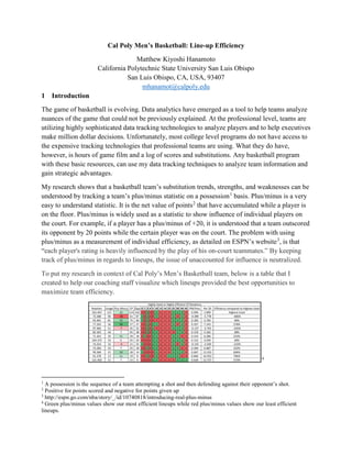
To put my research in context of Cal Poly’s Men’s Basketball team, below is a table that I
created to help our coaching staff visualize which lineups provided the best opportunities to
maximize team efficiency.
4
1
A possession is the sequence of a team attempting a shot and then defending against their opponent’s shot.
2
Positive for points scored and negative for points given up
3
http://espn.go.com/nba/story/_/id/10740818/introducing-real-plus-minus
4
Green plus/minus values show our most efficient lineups while red plus/minus values show our least efficient
lineups.
Rotation Usage Plus Minus CP Opp 0 1 3 4 5 10 13 14 23 25 30 34 42 PM/Poss Per 20 Efficiency compared to Highest Used
102.407 127 12 114 102 0 0 1 0 0 1 0 0 0 1 1 1 0 0.094 1.890 Highest Used
72.288 90 -26 61 87 1 0 1 0 0 1 0 0 0 1 0 1 0 -0.289 -5.778 -406%
92.401 81 15 75 60 1 0 1 0 0 0 0 0 0 1 1 1 0 0.185 3.704 96%
77.293 56 20 57 37 0 0 1 0 1 1 0 0 0 1 0 1 0 0.357 7.143 278%
97.406 51 -7 45 52 0 0 1 0 1 0 0 0 0 1 1 1 0 -0.137 -2.745 -245%
82.303 44 7 45 38 0 0 1 0 1 1 0 0 0 0 1 1 0 0.159 3.182 68%
71.263 35 11 29 18 0 1 0 0 1 1 0 0 0 1 1 0 0 0.314 6.286 233%
104.373 33 5 25 20 0 0 0 0 1 1 0 0 0 1 1 1 0 0.152 3.030 60%
74.254 32 -4 21 25 1 0 0 0 1 1 0 0 0 1 0 1 0 -0.125 -2.500 -232%
73.283 23 7 25 18 0 0 1 0 1 1 0 0 0 1 1 0 0 0.304 6.087 222%
99.368 21 14 28 14 1 0 0 0 0 1 0 0 0 1 1 1 0 0.667 13.333 606%
91.278 13 11 19 8 0 0 1 0 0 1 0 0 1 1 1 0 0 0.846 16.923 796%
121.403 11 7 13 6 0 0 0 0 1 1 0 0 0 0 1 1 1 0.636 12.727 573%
Highly Used or Highly Efficient CP Rotations
2. 2
From that table, we can interpret which lineups were favored in games5
, which lineups worked
throughout the season6
, and which lineups resulted in negative outcomes7
.
Additionally, by keeping track of the defensive alignments of a team and of their opponent, we
can understand which lineups operate most efficiently in and against certain types of defenses.
1.1 Research Question:
The focus of my study was to determine which groups of players on Cal Poly’s Men’s Basketball
team performed the most efficiently together.
• Unit of efficiency: I used plus/minus per possession as my unit of efficiency.
• Supplement: I also tracked and analyzed which groups of players were the most efficient
against different types of defenses.
2 Basketball Basics (Readers who are familiar with the game… skip to Section 2.4.)
If the reader is unfamiliar with the game of basketball, below are some guidelines of the game.
2.1 Objective: Score as many points as possible, while limiting your opponent to fewer
points. (You accomplish this by shooting the ball through your opponent’s hoop as many times
as you can.)
2.2 Rules:
• There are five players, per team, allowed on the court at one time.
o The five players form what will be referenced as a “line up.”
• When your team has the ball, you collectively have 35 seconds to attempt a shot at your
opponent’s hoop.
o If your team misses the shot and regains possession of the ball, your team has
another 35 seconds to attempt a shot.
5
This can be determined by the usage column
6
High positive plus/minus values provide a good indication of which lineups work. One can also compare the
efficiency of other highly used lineups to the starting lineup. Rotation 77.293 was a good example of a highly
efficient lineup that was used sparingly and could have been utilized more often.
7
Rotation 72.288 was our least efficient lineup on the year. This was a perfect example of how the eye test can
deceive you. The players who made up this lineup looked as though they would work great together, but the
numbers told another story.
Rotation Usage Plus Minus CP Opp 0 1 3 4 5 10 13 14 23 25 30 34 42 PM/Poss Per 5 Efficiency compared to Highest Used
92.401 17 7 17 10 1 0 1 0 0 0 0 0 0 1 1 1 0 0.412 2.059 Highest Used
102.407 13 1 15 14 0 0 1 0 0 1 0 0 0 1 1 1 0 0.077 0.385 -81%
72.288 8 6 13 7 1 0 1 0 0 1 0 0 0 1 0 1 0 0.750 3.750 82%
73.283 8 3 9 6 0 0 1 0 1 1 0 0 0 1 1 0 0 0.375 1.875 -9%
82.303 8 1 12 11 0 0 1 0 1 1 0 0 0 0 1 1 0 0.125 0.625 -70%
97.406 8 2 9 7 0 0 1 0 1 0 0 0 0 1 1 1 0 0.250 1.250 -39%
77.293 6 -2 6 8 0 0 1 0 1 1 0 0 0 1 0 1 0 -0.333 -1.667 -181%
72.145 5 -4 0 4 1 0 0 0 1 1 0 0 1 0 0 1 0 -0.800 -4.000 -294%
104.373 5 1 6 5 0 0 0 0 1 1 0 0 0 1 1 1 0 0.200 1.000 -51%
72.297 4 4 4 0 1 0 1 0 1 0 0 0 0 0 1 1 0 1.000 5.000 143%
74.254 4 -10 0 10 1 0 0 0 1 1 0 0 0 1 0 1 0 -2.500 -12.500 -707%
77.298 3 5 5 0 1 0 1 0 0 1 0 0 0 0 1 1 0 1.667 8.333 305%
Effectiveness of 1-3-1 Defense
3. 3
• While your team has the ball8
, you can score 1, 2, 3, or 4 points.
o Point value of a shot is determined by distance from the hoop. Occasionally,
players can earn extra opportunities to score points if there is an excessive amount
of contact endured while attempting a shot.
• While your opponent has the ball9
, your opponent has the same scoring opportunities.
• The two teams on the court play two 20 minutes halves in which they try to score against
one another as many times as possible.
• At the end of the 40 minutes of playing time, whoever has accumulated the most points,
wins.
o If there is a draw at the end of the 40 minutes of playing time, there are short
overtime periods in which the teams will play until there is a winner.
2.3 Types of Defenses:
1-2-2 Zone10 Man-to-Man11 1-3-1 Zone12
The purpose of positioning your players in different defensive alignments is to exploit the
weaknesses of your opponent. For example, zone type defenses are employed to increase the
difficulty of scoring close to the basket. Players who struggle to maintain efficient shooting
percentages far from the basket typically struggle against zone defenses.
2.4 Vocabulary to know:
• Possession: the sequence of your team attempting a shot and then defending against your
opponent’s shot.
• Plus/Minus: the net value of how many points your team scores while on offense and
how many points your opponent scores while you are on defense.
8
This will be referred to as offense.
9
This will be referred to as defense.
10
UC Santa Barbara uses the 1-2-2 defense frequently.
11
All basketball teams will run a man to man defense.
12
Cal Poly specialized in the 1-3-1 defense.
4. 4
3 Data Collection
3.1 Note to the Data Collector
The key to an accurate analysis of one’s team is meticulous data entry and uniformly formatted
data. You will need to keep your information in a common format in order for you to have
interpretable information as the season progresses. It is important to note that one game of data
will not tell you much about how your team will perform throughout the season. Ten games,
however, should be a sizeable enough sample to make informed decisions on how different
lineups are performing. I highly recommend using Microsoft Excel to organize your data and to
expedite the summary statistic process. I also recommend recording each game in a separate
Excel file. To make all of my recordings uniform, I created a template to use for each game.
After I finished recording each game, I moved all of the data I recorded into a larger spreadsheet
that served as my database.
3.2 Method
I created a database of every single possession from this past season, from scratch. For each
individual possession, I included which players from our team were in the game, how many
points we scored, how many points our opponent scored, which defensive alignment we were in,
and which defensive alignment our opponent was in.
3.3 Player Tracking
Keeping track of who is in the game is easy. Give the player a value of one, if he or she is in the
game, and a value of zero, if he or she is out of the game. You will only need to change your
inputs when there is a substitution.
3.4 Point Tracking
Knowing which possession points were scored in becomes challenging when there are offensive
rebounds involved. To show that a team did not score in a possession, I assign “Pts Offense” a
value of zero. If there is an offensive rebound, I skip to the next line and treat the next shot as a
new possession.13
13
Be careful during this part of the data entry because the way you have entered the scoring information now
switches in order. If your opponent was shooting first in a possession and your team gets an offensive rebound on
their shot attempt, your team’s scoring information will be now entered before your opponent’s. This seems like a
minor detail now, but it can get very confusing when you are in the middle of a game and there is no stoppage in
play.
0 1 3 4 5 10 13 14 23 25 30 34 42
1 1 1 0 0 0 0 0 0 1 1 0 0
Team Possession Half P.M Rotation Indicator CP Man CP 13 CP 23 CP 12 Opp Man Opp 23 Opp 12 Opp 13 Pts Offense Pts Against
Nevada 1 1 2 59.291 1 0 0 0 1 0 0 0 2 0
5. 5
3.5 Error Proofing
To ensure that I am only observing five players on the court at the same time, I used an if-else
statement to tell me whether or not there are five players in the game.14
The line of code could be
as simple as asking Excel to tell you “OK” if the sum of all players in a row is equal to five.
Also, be sure to keep track of the score while recording your data. This is incredibly useful in
situations where you realize your final score doesn’t add up and you want to find the exact
possession where you may have entered the wrong point value. I recommend creating two
columns that keep a running tally of the “Pts Offense” and “Pts Against.”
3.6 Unique Indicator Variables
The picture below shows how I tagged each lineup with an individual rotation indicator variable.
To create a unique indicator variable, I used Excel’s sumproduct function. This function, in
context of my database, adds up each of the numbers of the players in the lineup. I had originally
used just the players’ numbers (with no added decimals) in the sumproduct function, but ran
across the problem of overlap among certain combinations of players. For example, the sum of
players 0, 5, 13, 25, and 34 would have the exact same rotation indicator variable15
as the players
3, 5, 10, 25, and 34. This was only one of numerous instances that this problem arose. What I did
to combat this problem was add a random three digit decimal to the end of the players’ numbers.
At first, I tried to increase the three digit numbers in a specific order, but ran into overlap a
second time. Choosing random numbers was my solution to removing overlap. There are more
statistically sound ways to make sure there is a 0% possibility of overlap and I will look to apply
those methods at a later date.
14
It is amazing how easy it is to put four or six players on the court at one time.
15
Rotation indicator = 77
Rot OK CP Opp
OK 2 0
OK 3 2
OK 5 2
OK 5 2
0.001 1.020 3.040 4.050 5.006 10.007 13.080 14.090 23.001 25.110 30.120 34.130 42.140
1 1 1 0 0 0 0 0 0 1 1 0 0
Rotation Indicator
59.291
6. 6
3.7 Defense Tracking
This aspect of the data tracking process requires hours of practice and a keen eye. In the Big
West conference, there are only four types of defenses that teams play.
1) Man-to-Man (Each player on defense is matched up with a player on offense. This type
of defense is used by every team in the country.)
2) 2-3 Zone (Each player on defense is responsible for a specific zone on the court. There
are typically two guards around the free throw line, a center in the middle of the paint,
and two forwards in the lower corners. This defense is used most often by teams with a
very tall center16
.)
3) 1-2-2 Zone (Like the 2-3 zone, each player is responsible for a zone on the court. This
alignment however has a forward and a center protecting the hoop, two wings near the
free throw line, and a guard pressuring near the top of the key and dropping down to help
in the middle of the defense.)
16
A good example of this type of team is UC Irvine. They have a 7’8” center who is very effective as a rim
protector.
7. 7
4) 1-3-1 Zone (The 1-3-1 zone operates similarly to the other zones, but there is usually a
long-armed, athletic wing at the very top of the formation. He is there trying to pressure
the ball as it gets thrown from one side of the court to the other side. There are three
players lined up in the middle of the court trying to prevent a pass to the corners nearest
the basket. The player on the bottom of the formation is responsible for running and
contesting shots in the corners.)
Tracking defensive alignments is a tedious process. There are no services that will track this data
for you. A trick that I found very useful was to watch how the defense responds to a cutting
player. The initial cut will let you know if the defense is in Man-to-Man or in a type of zone. If a
defender follows the cutting player everywhere around the court, you can be certain that the
defense is in man. If the defender of the cutter does not follow the cutter and another player picks
up the player at the end of the cut, the defense is probably in zone. The only way to get good at
tracking defense is by watching film and picking up on tendencies of teams.17
3.8 Summary of Data Collection/Tips and Tricks
Tracking all of this information in real time is not an easy process. Offensive rebounds, quick
lineup changes, and changing defenses are not easy variables to monitor and log. When the data
collector cannot be at a game, using a school’s play by play18
makes the logging of points and
substitutions easy. In the play by play, every substitution is listed and every score is logged. The
only thing you need to do is record the information in a numerical format. Once you have
documented every point and lineup change, all you have to do is watch the film and mark which
defense the teams are in during their possessions. Play by plays are not always one hundred
percent accurate, but most are near perfect. Understanding how the game flows will help you
correct errors and understand when you need to make an adjustment.
17
There are even teams, such as CSU Northridge, that will change their defense halfway through a play. Their coach
would actually make a loud whistle noise and his players would switch from their zone defense to man-to-man.
18
This is usually found on a school’s athletics website.
8. 8
4 Analysis
Once you have all of your data recorded and everything is compiled into a single spreadsheet,
you will want to create a PivotTable to analyze and produce summary statistics.
4.1 How to build a PivotTable
1) Highlight everything on the spreadsheet that contains all of your recorded data. (Ctrl+a)
2) Insert -> Pivot Table (Choose new worksheet)
3) Filters (Drag the variables that you want to filter your data by):
- Possession
- Win/Loss
- Location
- Half
- All Player numbers
- All Defenses
- Team
4) Columns: (Don’t Touch)
5) Rows: Rotation Indicator
6) Values:
- Counts of rotation indicators
- Sum of +/-
- Sum of Pts Offense
- Sum of Pts Against
9. 9
The great thing about pivot tables is how easy it makes the process of analyzing your data.
• You can sort your data by highest scoring lineups to lowest scoring lineups.
• You can use Excel’s conditional formatting option to color coordinate high and low
performing lineups.
• You can filter out players who are no longer of interest in your rotations.19
• NOTE: I ran into the issue of figuring out who was in the lineups listed in the PivotTable.
o To solve this issue, I copied all of the data from my database sheet into a separate
sheet that I called Rotation Match. In this sheet, I sorted all of the data in order of
the value of the rotation indicator variable.20
o Going back to the PivotTable sheet, I used a vlookup function to pull the 0 and 1
values from the Rotation Match sheet.
Example syntax: =VLOOKUP($G18,'Rotation Match'!$G$2:$S$1310,2)
(Full database spreadsheet layout)
(Rotation Match spreadsheet)
19
This is especially useful if a player becomes ineligible during a season or you lose a player to injury. Instead of
panicking about figuring out how to use only relevant data, you can just filter the player out of your table.
20
Make sure the variable Rotation Indicator Variable is in the column next to the player numbers.
10. 10
4.2 Summary of Analyses
Sort all of our lineups based on overall efficiency. How do these lineups compare to the
team average? (Sort your lineups by most frequently used and divide their plus/minus values by
the amount of times each of the lineups were used.)
How has the team performed against zone defense? (In the PivotTable, set your opponent’s
defense filter of man-to-man to zero. The resulting observations should be all of your team’s
possessions against a type of zone defense.21
)
21
If you want to be more specific, you can filter your opponent’s defense filter to only include the defense you are
interested in.
0.41
0.33
0.23
0.12 0.11 0.09 0.06
-0.07 -0.07
-0.15
-0.30-0.40
-0.30
-0.20
-0.10
0.00
0.10
0.20
0.30
0.40
0.50
Overall Plus/Minus
Plus Minus per possession Average Plus Minus
0.89
-0.07 -0.11
-0.38 -0.43 -0.46
-0.70 -0.73 -0.74
-1.50
-1.00
-0.50
0.00
0.50
1.00
77.293 92.401 77.298 67.287 102.407 74.254 121.403 75.361 72.288
Plus/Minus against Zone
Plus Minus per possession Average Plus Minus
11. 11
Show only the summary statistics starting from a certain point in time to now. (Our head
coach made an adjustment to his coaching strategy midway through our season. All you have to
do is filter which games were played in the time frame after the adjustment in coaching strategy.)
- It will be beneficial to label each of your data files in chronological order. I chose to
list each of mine by what date the game was played on and who the game was
against.
o (Ex. 2015.3.7 CP. UC Santa Barbara 2.xlsx)
Are there any lineups that we use frequently that are not effective?
Our second highest used lineup has a large, negative plus/minus value of -26. This statistic
should be very surprising to followers of our team. The players featured in this lineup are all very
good players. The lineup included a senior leader, a dynamic slasher, a prominent point guard,
and our two staple big men. What seemed to bother this lineup was a lack of spacing on the
basketball court. The skills of the players overlapped and the lineup efficiency suffered.
Which lineup is the most effective in our 1-3-1 defense?
Based on our defensive tracking data, lineup 92.401 proved to be our most effective 1-3-1 lineup.
Lineup 121.403 was more efficient in regards to ratio of plus/minus to frequency of usage, but it
had nearly 20 fewer observations. In this analysis, I chose to reward lineups who were used more
frequently because getting defensive stops does not get easier with an increase in attempts. My
efficiency statistic was calculated by dividing plus/minus by the frequency of the lineup. To
weight the efficiency, I multiplied the percent usage by the efficiency statistic to get a better
indicator of how well the lineup performed.
Row Labels Count of Rotation Indicator Count weight Sum of P.M Efficiency Weighted Efficiency Sum of Pts Offense Sum of Pts Against 0 1 3 4 5 10 13 14 23 25 30 34 42
92.401 30 24% 8 0.267 0.065 29 21 92.401 1 0 1 0 0 0 0 0 0 1 1 1 0
67.287 20 16% 1 0.050 0.008 30 29 67.287 1 0 1 0 1 0 0 0 0 1 0 1 0
102.407 17 14% 3 0.176 0.024 19 16 102.41 0 0 1 0 0 1 0 0 0 1 1 1 0
75.361 14 11% 3 0.214 0.024 11 8 75.361 1 0 1 0 0 0 1 0 0 1 0 1 0
97.406 13 10% 5 0.385 0.040 15 10 97.406 0 0 1 0 1 0 0 0 0 1 1 1 0
121.403 11 9% 7 0.636 0.056 12 5 121.4 0 0 0 0 1 1 0 0 0 0 1 1 1
91.284 10 8% 2 0.200 0.016 10 8 91.284 1 0 0 0 1 1 0 0 0 0 0 1 1
74.254 9 7% -12 -1.333 -0.097 6 18 74.254 1 0 0 0 1 1 0 0 0 1 0 1 0
12. 12
How can we put ourselves in the best position to win?
(Substitution patterns and scoring trends)
March 12, 2015 was the date of Cal Poly’s first round Big West Tournament game. They were
scheduled to play UC Santa Barbara, a team that they were defeated by five days prior. Days
before our tournament game, I decided to try my data tracking method on our opponent. I used
all of UC Santa Barbara’s conference games as my data source and was able to gain an
understanding of UCSB’s substitution patterns and the scoring tendencies of their team.
Based on the results in the substitution patterns table, I was able to interpret that UC Santa
Barbara was a team that put the majority of their effort in getting ahead early in the game. Also, I
was able to interpret that their starting lineup was essentially their only efficient scoring lineup.
Over the course of conference play, their starters were +25 in the first 20 possessions of the game
and +34 in the entire first half. The same group of players, however, were only +7 in the second
half of games. The reason this kind of information is valuable is because starting lineups tend to
play the majority of the minutes in a game. Understanding the opponent’s production patterns
can definitely give your team a strategic advantage. The summary statistics told us that if you
can manage to keep the game close throughout the first half, you can take advantage of their
lower levels of efficiency at the end of game.
Possessions 1-20 Start - first half of first half
Rotation Usage Plus Minus SB Opp % Played 0 1 2 3 11 12 13 15 21 24 31 44
76.152 63 25 64 39 53% 0 0 1 1 0 0 0 1 0 1 1 0
74.851 11 1 7 6 9% 0 1 0 1 0 0 0 1 0 1 1 0
64.302 5 -3 2 5 4% 0 1 1 0 0 0 0 1 1 1 0 0
74.211 5 -4 5 9 4% 0 1 1 0 0 0 0 1 0 1 1 0
76.888 5 -1 2 3 4% 0 0 0 1 0 0 1 1 1 1 0 0
120 Possessions
Possessions 21-37 2nd half of first half - half time
Rotation Usage Plus Minus SB Opp % Played 0 1 2 3 11 12 13 15 21 24 31 44
76.152 21 9 25 16 21% 0 0 1 1 0 0 0 1 0 1 1 0
64.852 17 -6 11 17 17% 0 0 1 1 0 0 1 1 0 0 1 0
62.911 16 -2 16 18 16% 0 1 1 0 0 0 1 1 0 0 1 0
56.24 6 1 5 4 6% 0 0 1 1 1 0 0 1 0 1 0 0
86.797 6 -4 4 8 6% 0 0 0 1 0 0 1 1 0 1 1 0
102 Possessions
Possessions 38-60 Half time - first half of second half Most likely to see Childress, Taylor, Brewe, Beeler
Rotation Usage Plus Minus SB Opp % Played 0 1 2 3 11 12 13 15 21 24 31 44
76.152 59 4 59 55 43% 0 0 1 1 0 0 0 1 0 1 1 0
74.851 18 -8 10 18 13% 0 1 0 1 0 0 0 1 0 1 1 0
66.245 12 -3 9 12 9% 0 0 1 0 1 0 1 1 0 1 0 0
51.984 9 1 12 11 7% 0 1 0 1 1 0 0 1 1 0 0 0
114.006 5 -2 2 4 4% 0 1 0 0 0 0 1 0 0 1 1 1
138 Possessions
Possessions 61-Finish 2nd half of 2nd Half - End of Game
Rotation Usage Plus Minus SB Opp % Played 0 1 2 3 11 12 13 15 21 24 31 44
76.152 22 3 14 11 18% 0 0 1 1 0 0 0 1 0 1 1 0
57.898 10 5 11 6 8% 0 0 1 1 0 0 1 1 0 1 0 0
45.952 8 5 8 3 7% 0 1 1 1 0 0 0 1 0 1 0 0
74.851 8 3 10 7 7% 0 1 0 1 0 0 0 1 0 1 1 0
54.187 7 3 4 1 6% 0 0 1 1 1 0 1 0 0 1 0 0
56.597 7 1 4 3 6% 0 1 0 1 0 0 1 1 0 1 0 0
122 Possessions
482 Total
Most Likely to see Smith in during this time
Most Likely to see Smith in during this time
Most Likely to see Brewe in during this time
13. 13
Game Results:
Actual substitutions:
As predicted, Santa Barbara’s starters were the only efficient scoring group of players on their
team. They were played 46 percent of the game together and finished with a plus/minus of +8.
An interesting observation was that the starting lineup followed their second half trend of
dropping in efficiency. They dropped from +7 in the first half all the way down to +1 in the
second half. Also, the pattern of UCSB’s substitutions were very similar to the predictions made
prior to the game. The only inconsistency was the increase in playing time of player number 1
over player number 13. This inconsistency could be due to the absence of player number 13 from
the previous game.
Cal Poly was in a position to win this game. With two minutes to go, Cal Poly was down 50 to
52 and had possession of the ball. They had two attempts to make a shot and were unsuccessful.
Santa Barbara had also missed a shot and turned the ball over in this timespan. With 50 seconds
to go, Santa Barbara had possession of the ball and Cal Poly needed to get a defensive stop. Our
best defensive lineup22
, according to the data, was inserted into the game and successfully forced
a turnover. With 30 seconds remaining, Cal Poly had a shot to tie or win the game.
22
Rotation Indicator: 92.401
Rotation Indicator Count of Rotation Indicator Sum of +/- Sum of Pts Offense Sum of Pts Against 0 1 2 3 11 12 13 15 21 24 31 44
52.906 4 -1 2 3 52.906 0 1 1 1 0 0 0 1 0 0 1 0
63.194 4 -3 3 6 63.194 0 0 1 1 1 0 0 1 0 0 1 0
74.851 14 -2 11 13 74.851 0 1 0 1 0 0 0 1 0 1 1 0
74.947 7 1 4 3 74.947 0 1 0 0 0 0 1 1 1 1 0 0
76.152 32 8 29 21 76.152 0 0 1 1 0 0 0 1 0 1 1 0
81.143 1 0 2 2 81.143 0 1 0 1 0 0 0 0 1 1 1 0
94.092 3 2 2 0 94.092 0 1 0 1 0 0 0 0 1 1 0 1
103.361 3 1 1 0 103.361 0 1 1 0 0 0 0 0 0 1 1 1
106.038 2 -2 0 2 106.038 0 0 0 1 0 0 1 0 1 1 0 1
Grand Total 70 4 54 50
Possessions 1-20
Rotation Usage Plus Minus SB Opp % Played 0 1 2 3 11 12 13 15 21 24 31 44
74.947 6 1 4 3 30% 0 1 0 0 0 0 1 1 1 1 0 0
76.152 11 1 6 5 55% 0 0 1 1 0 0 0 1 0 1 1 0
103.361 3 1 1 0 15% 0 1 1 0 0 0 0 0 0 1 1 1
Possessions 20 3
Possessions 21-37
Rotation Usage Plus Minus SB Opp % Played 0 1 2 3 11 12 13 15 21 24 31 44
52.906 4 -1 2 3 24% 0 1 1 1 0 0 0 1 0 0 1 0
63.194 4 -3 3 6 24% 0 0 1 1 1 0 0 1 0 0 1 0
74.947 1 0 0 6% 0 1 0 0 0 0 1 1 1 1 0 0
76.152 8 6 11 5 47% 0 0 1 1 0 0 0 1 0 1 1 0
Possessions 17 2
Possessions 38-60
Rotation Usage Plus Minus SB Opp % Played 0 1 2 3 11 12 13 15 21 24 31 44
74.851 5 3 7 4 22% 0 1 0 1 0 0 0 1 0 1 1 0
76.152 12 -1 10 11 52% 0 0 1 1 0 0 0 1 0 1 1 0
81.143 1 0 2 2 4% 0 1 0 1 0 0 0 0 1 1 1 0
94.092 3 2 2 0 13% 0 1 0 1 0 0 0 0 1 1 0 1
106.038 2 -2 0 2 9% 0 0 0 1 0 0 1 0 1 1 0 1
Possessions 23 2
Possessions 61-Finish
Rotation Usage Plus Minus SB Opp % Played 0 1 2 3 11 12 13 15 21 24 31 44
74.851 9 -5 4 9 90% 0 1 0 1 0 0 0 1 0 1 1 0
76.152 1 2 2 10% 0 0 1 1 0 0 0 1 0 1 1 0
Possessions 10 -3
Total 70
Plus/Minus
Half time - first half of second half
2nd half of 2nd Half - End of Game
2nd half of first half - half time
Start - first half of first half
Plus/Minus
Plus/Minus
Plus/Minus
Prediction: Most Likely to see Smith in during this time
Prediction: Most Likely to see Brewe in during this time
Prediction: Most likely to see Childress, Taylor, Brewe, Beeler
Prediction: Most Likely to see Smith in during this time
14. 14
Cal Poly did not end up winning this basketball game.23
Despite limiting Santa Barbara’s first
half scoring and controlling the pace of the game, Santa Barbara prevailed. The key thing to
remember, however, is that Cal Poly was in a position to win this game.
5 Conclusion
Basketball analytics are revolutionizing how teams are able to form game strategies. What I have
done is break the game of basketball down to its purest form of scoring and defending. My data
tracking methods and simple analyses have enabled our team to gain an advanced understanding
of team tendencies, strengths, and weaknesses.
Analytics will never be able to take the place of a coach, replace basketball instinct, or guarantee
the success of a team. It can, however, help coaches understand pieces of the game where
intuition cannot provide the answer. It is my hope that my framework for tracking a team’s
production can help basketball programs understand the basics of advanced metrics and provide
the building blocks for finding strategic advantages.
23
Final score was 54-50.
0
10
20
30
40
50
60
1 4 7 10 13 16 19 22 25 28 31 34 37 40 43 46 49 52 55 58 61 64 67 70
Cal Poly vs. UCSB
3/12/2015
SB CP
15. 15
6 Acknowledgements
I would like to thank the following professors for their assistance on this project: Pratish Patel,
Larry Gorman, Ziemowit Bednarek, Peter Chi, and Gary Hughes. I am very gracious for all of
your the suggestions and input.
Also, thank you to the Cal Poly Men’s Basketball program for giving me the resources to pursue
this project.
7 Sample Report
Once I had a firm understanding of how to create visual representations the data I was collecting,
I decided to create a scouting report for our last regular season game against UC Santa Barbara.
There was not enough time to create a full report for our Big West tournament game. Included
are examples of tables and graphs that can help visualize the performance of lineups. Also, there
are interpretations of the visuals to help coaches understand what they was looking at.
17. Game Recap and Notes:
- 1st Half Possessions: 38 vs. 52 2nd Half Possessions (Pace of game was more in their favor toward the end)
- SB used their 1-2-2 on 28 possessions:
o We were only able to convert 19 points on 28 possessions.
o If we were to looking to get at least 1 point per possession then we converted on 68% of that goal.
o Lineups facing the 1-2-2 unfortunately ended up allowing 27 points on those same 28 possessions.
- Not sure if this was purely a random shift in momentum, but #0 (Hunter Ford) was the addition to SB’s
rotation that pushed them to the lead. (Reference: Ford, Vincent, Harmon, Al, Bryson lineup) He was also
featured in other lineups that performed fairly well.
o He is a bottom level guy on Synergy’s report, but his addition on the court (29% of the game and a
+13 while he was on the court) was a difference maker in our previous game.
- SB seemed prepared for 13. We attempted to run the defense on 19 possessions and they were able to
score 19 points.
o SB converted every time 13 dropped too low. (Three middle guys sank too low into the key)
0
10
20
30
40
50
60
1 9 17 25 33 41 49 57 65 73 81 89
CP vs. SB 1.1.2015
CP SB
20. Santa Barbara Rotations
• Santa Barbara’s scoring was well distributed among their lineups.
• Starting line-up’s +/- was (-7) in our previous game. (This could be attributed to us having ideal matchups against
that lineup.
-3
-2
-1
0
1
2
3
1 2 3 4 5 6 7 8 9 10 11 38 39 40 41
Vincent, Harmon, Al, Brewe,
Bryson
CP SB
-3
-2
-1
0
1
2
3
29 30 31 32 33 34 35 36 37
Vincent, Harmon, Taylor, Al,
Brewe
CP SB
-3
-2
-1
0
1
2
69 70 71 72 73 74 75 76 77 78 79 80 81 82
Ford, Vincent, Harmon, Al,
Bryson
CP SB
-2
-1
0
1
2
3
21 22 23 24 25
Childress, Taylor, Al, Green,
Beeler
CP SB
21. Cal Poly Rotations
• In the 12 possessions Ant was in, SB did not score a basket. We were also able to capitalize on offense and score 7
points in those 12 possessions.
0
0.5
1
1.5
2
2.5
3
19 20 21 22 23 54 55 56 57 58 59 60
Reese, Ridge, Mike, Brian, Ant
Pts O Opp
0
0.5
1
1.5
2
65 66 67 79 85 87
Maliik, Reese, Ridge, Joel, Brian
Pts O Opp
-3
-2
-1
0
1
2
68 69 70 71 72 73 74 75 76 77 78
Dave, Maliik, Ridge, Mike,
Brian
Pts O Opp
-3
-2
-1
0
1
2
3
61 62 63 64
Liik, Reese, Ridge, Joel, Mike
Pts O Opp
24. UCSB Roster
No. Name Pos. Cl. Ht. Wt. Hometown/High School
0 Hunter Ford Guard Sophomore 6-3 180 Roseville, Calif./Oakmont HS
1 Eric Childress Guard Sophomore 6-0 175 Hawthorne, Calif./Leuzinger HS
2 Gabe Vincent Guard Freshman 6-3 190 Stockton, Calif./St. Mary's
3 Zalmico Harmon Guard Senior 6-0 185 Washington, D.C./Ballou High School
5 Tide Osifeso Guard Freshman 5-10 145 Rancho Cucamonga, Calif./Los Osos, Calif.
11 T.J. Taylor Guard Junior 5-9 160 Oakland, Calif./Oakland HS
12 Alex Hart Forward Sophomore 6-10 215 Kelowna, British Columbia, Canada/Immaculata High School
13 DaJuan Smith Guard Junior 6-3 175 Abbeville, La./Abbeville HS
14 Ami Lakoju Forward Freshman 6-8 265 Harlem, N.Y./St. Luke's School
15 Alan Williams Center Senior 6-8 265 Phoenix, Ariz/North HS
20 Logan Louks Guard Junior 6-2 175 Danville, Calif./San Ramon Valley HS
21 Mitch Brewe Forward Junior 6-8 242 Seattle, Wash./Seattle Preparatory School
23 Sam Walters Guard Freshman 6-2 170 Soquel, Calif./Soquel HS
24 Michael Bryson Guard Junior 6-4 201 Sacramento, Calif./Foothill HS
25 Justin Burks Forward/Guard Freshman 6-6 210 Las Vegas, Nev./Arbor View HS
31 John Green Guard Junior 6-5 180 Oakland, Calif./Westwind Prep Academy (Phoenix)
32 J.D. Slajchert Forward Freshman 6-6 215 Oak Park, Calif./Phillips Exeter Academy
43 Joey Goodreault Guard Freshman 6-3 175 Orinda, Calif./Miramonte HS
44 Sam Beeler Forward Junior 6-10 210 Poway, Calif./Poway HS
25. ** Last note:
- I am still unsure why this lineup doesn’t work, but it has not performed well over the course of the season…
• The only game that this group was used in, that resulted in a win, was the very first
conference game against Hawaii.
-3
-2
-1
0
1
2
3
Hawaii1
CSUF1
UCR1
UCR1
UCI1
UCD1
UCD1
UCD1
UCD1
UCD1
UCD1
UCD1
UCD1
UCD1
UCD1
UCD1
UCD1
UCD1
UCD1
UCD1
Hawaii2
Hawaii2
Hawaii2
Hawaii2
Hawaii2
Dave, Maliik, Ridge, Joel, Brian
CP Opponent