М.Г.Гоман, А.В.Храмцовский (1998) - Использование методов непрерывного продолжения решений и бифуркационного анализа для синтеза систем управ

М.Г.Гоман, А.В.Храмцовский "Использование методов непрерывного продолжения решений и бифуркационного анализа для синтеза систем управления", Phil.Trans.R.Soc.Lond. A (1998) 356, 2277-2295 M.G.Goman and A.V.Khramtsovsky "Application of continuation and bifurcation methods to the design of control systems", Phil.Trans.R.Soc.Lond. A (1998) 356, 2277-2295 In this paper the continuation and bifurcation methods are applied to aircraft nonlinear control design problems. The search for the recovery control from spin regimes is based on the minimization of an energy-like scalar function constrained by the aircraft's equilibria conditions. The design of a global stability augmentation system for severe wing-rock motion is performed by using bifurcation diagrams for equilibrium and periodical modes. The nonlinear control law, which totally suppresses wing-rock motion, is derived, taking into account both local stability characteristics of aircraft equilibrium states and domains of attraction, along with the requirement that all other attractors be eliminated.

Recommended
Recommended
More Related Content
What's hot
What's hot (20)
Similar to М.Г.Гоман, А.В.Храмцовский (1998) - Использование методов непрерывного продолжения решений и бифуркационного анализа для синтеза систем управ
Similar to М.Г.Гоман, А.В.Храмцовский (1998) - Использование методов непрерывного продолжения решений и бифуркационного анализа для синтеза систем управ (20)
More from Project KRIT
More from Project KRIT (18)
Recently uploaded
Recently uploaded (20)
М.Г.Гоман, А.В.Храмцовский (1998) - Использование методов непрерывного продолжения решений и бифуркационного анализа для синтеза систем управ
- 1. Application of continuation and bifurcation methods to the design of control systems By M. G. Goman1,2 and A. V. Khramtsovsky1 1 Central Aerohydrodynamic Institute (TsAGI), Zhukovsky 140160, Russia 2 Department of Mathematical Sciences, Faculty of Computing Science and Engineering, De Montfort University, Leicester LE1 9BH, UK The use of nonlinear dynamics theory for the analysis of aircraft motion and the assessment of aircraft control systems is well known. In this paper the continuation and bifurcation methods are applied to aircraft nonlinear control design problems. The search for the recovery control from spin regimes is based on the minimization of an energy-like scalar function constrained by the aircraft’s equilibria conditions. The design of a global stability augmentation system for severe wing-rock motion is performed by using bifurcation diagrams for equilibrium and periodical modes. The nonlinear control law, which totally suppresses wing-rock motion, is derived, taking into account both local stability characteristics of aircraft equilibrium states and domains of attraction, along with the requirement that all other attractors be eliminated. Keywords: aircraft spin; recovery control; wing-rock motion; domains of attraction; bifurcation diagrams; reconfigurable control law 1. Introduction The analysis of aircraft nonlinear dynamics problems by using bifurcation methods has been investigated over the past 20 years. The results of such work are pub- lished in the literature both for open-loop and closed-loop aircraft models (Mehra et al. 1977, 1978, 1979; Carroll & Mehra 1982; Guicheteau 1982, 1990; Zagainov & Goman 1984; Planeaux & Barth 1988; Planeaux et al. 1990; Jahnke & Culick 1988, 1994; Lowenberg 1997; Liebst & DeWitt 1997; Littleboy & Smith 1997; Goman & Khramtsovsky 1997; Goman et al. 1997). The bifurcation methods were used mostly like methods of nonlinear dynamics analysis and assessment of control laws in the case of closed-loop aircraft models. Extending the flight envelope to high angle-of-attack (AOA) regions presents a big challenge in control-system design for modern and advanced manoeuvrable air- craft. At high AOA, the aerodynamic characteristics are essentially nonlinear, con- trol authorities of aerodynamic surfaces and other types of effectors are limited, and actuators provide additional constraints such as deflection limits and rate saturation. The existing multivariable control-law design techniques, such as nonlinear dynam- ic inversion (NDI), H∞ and µ-synthesis, are unable to take explicit account of all the important nonlinearities of aircraft mathematical models (Lane & Stengel 1988; Adams & Banda 1993; Goman & Kolesnikov 1997). In engineering practice, the lack of methods for nonlinear synthesis is usually compensated for by extensive numerical simulation of closed-loop system dynamics and empirical selection of the feedback Phil. Trans. R. Soc. Lond. A (1998) 356, 2277–2295 Printed in Great Britain 2277 c 1998 The Royal Society TEX Paper
- 2. 2278 M. G. Goman and A. V. Khramtsovsky gains and control-system parameters to obtain desirable handling qualities and stabil- ity characteristics. The qualitative bifurcation methods used in Goman et al. (1996) for maximizing the stability region of the closed-loop system, showed their potential in the control-law design process. The main object of the current paper is to demonstrate that qualitative meth- ods of nonlinear closed-loop system computational analysis with any type of con- troller (which usually leaves a set of free parameters in the derived control laws) can be efficiently applied to control system design. In this paper, the continuation and bifurcation diagram methods for equilibria and steady periodical motions, along with numerical study of their domains of attraction, are considered as basic tools for control interconnection and feedback-gains scheduling depending on state variables. All computations in the paper are performed by using a mathematical model for a hypothetical aircraft (Goman et al. 1995), whose aerodynamic characteristics are similar to the aerodynamic characteristics of many existing combat aircraft. This aircraft possesses severe wing-rock motion and flat-spin regimes due to aerodynamic asymmetry in yaw. The recovery control from flat-spin modes and wing-rock motion suppression by proper scheduling of feedback gains on state variables are presented to demonstrate the proposed control design methods. 2. Aircraft mathematical model The six-degrees-of-freedom equations of motion of a rigid-body aircraft with constant mass and inertia (under some physical assumptions), can be reduced to an eighth- order autonomous system of ordinary differential equations, which depends on the control parameters: dx dt = F (x, δ), (2.1) where x = (α, β, p, q, r, V, θ, φ) ∈ R8 , is the state vector composed of AOA, sideslip, body roll, pitch and yaw rates, velocity, pitch and bank angles, and δ =(ϕ, η, δa, δr, T) ∈ R4 is the control vector composed of mean and differential stabilator deflections, aileron and rudder deflections and thrust, (the prime denotes vector transposition). The steady-state regimes of this open-loop system, which are the vertical spiral trajectories, are defined by its equilibrium solutions, when control parameters are fixed or varied slowly. The vector function on the right-hand side of (2.1) is composed of kinematic, inertial and aerodynamic terms, the latter being dependent on aircraft configuration. Aerodynamic-model development is a special problem for each aircraft, and usually requires expensive and time-consuming analysis. A control-system mathematical model is added to the aircraft motion equations (2.1) as follows, dδ dt = Fc(x, δ, k, s), (2.2) where the vector-function, Fc, is determined by the structure of control laws, s = (xe, xa, xr, . . . ) is a control vector with stick and pedal deflections, and vector k is composed of feedback gains and parameters defining control-system constraints like actuator deflection limits and rate saturation. Phil. Trans. R. Soc. Lond. A (1998)
- 3. Continuation and bifurcation methods for control system design 2279 The state of the closed-loop system, described by a combination of (2.1) and (2.2), is extended by aerodynamic control deflections and thrust, i.e. z = (α, β, p, q, r, V, θ, φ, ϕ, η, δa, δr, T) . For example, to determine the equilibrium states of a closed-loop system, the follow- ing joint set of equations (2.3) should be used, F (x, δ) = 0, Fc(x, δ, k, s) = 0. (2.3) The elements of vectors x and δ are unknown variables now, and vectors s and k define the set of parameters. Note that the closed-loop system (2.3) possesses only a subset of the whole set of equilibrium solutions of the open-loop system (2.1), and the continuation of its equilibrium solutions with control parameters s, may lead to the ‘sharp’-fold bifurcation points when control surfaces enter on their deflection limits. (a) Representation of aerodynamic characteristics The aerodynamic model for high-incidence conditions is usually formulated by using experimental data obtained in a wind tunnel on the facilities for static, forced- oscillation and rotary balance tests (AGARD 1990). The proper combination of these experimental data for different flight conditions is very important for the adequacy of the mathematical model. The conventional representation of aerodynamic coefficients by using body axes angular rates p, q and r is consistent only when aerodynamic coefficients can be represented by linear dependencies on angular rates. Such representation is valid for small disturbed rectilinear flight paths. The spatial aircraft motion with intensive rotation at high AOA may strongly influence vortical and separated flow, and, as a consequence, the aerodynamic coefficients become nonlinear functions on an air- craft coning rate. In such a case, another characteristic motion parameter may be introduced for the representation of aerodynamic coefficients. In particular, the force and moment components resolved in the body-axes system can be represented as the functions on angular velocity components resolved in wind-body-axes system (the longitudinal axis coincides with the velocity vector, and the vertical axis is in the plane of an aircraft symmetry). The projections of the angular rate vector onto the wind-body axes are suitable for describing the disturbances with respect to pure conical motion. The roll rate in wind-body axes, i.e. pw = (p cos α + r sin α) cos β + q sin β, defines the rate of conical rotation, similar to the angular rate in rotary balance tests, and can be naturally used for the representation of nonlinear dependence on coning rate. Two other projections, qw = −(p cos α + r sin α) sin β + q cos β and rw = r cos α − p sin α, define both the unsteadiness and spirality of motion: ˙α = (qw − qwsp )/ cos β, ˙β = −rw + rwsp . The values of qwsp and rwsp are the wind-body angular rates in steady-state spiral motion, and their non-dimensional values, (qwsp ¯c/2V ) and (rwsp b/2V ), are usually negligible. Phil. Trans. R. Soc. Lond. A (1998)
- 4. 2280 M. G. Goman and A. V. Khramtsovsky Assuming that disturbances of the pure conical motion are small, the following representation of the aerodynamic coefficients can be used (i = X, Y, Z, l, m, n): Ci = CiRB α, β, pwb 2V , δ + Ciqw qwc 2V + Ci ˙α ˙α¯c 2V + Cirw rwb 2V + Ci ˙β ˙βb 2V = CiRB (α, β, pw, δ) + Ciqw + Ci ˙α cos β qw¯c 2V + (Cirw − Ci ˙β ) rwb 2V − Ci ˙α qwsp ¯c 2V cos β + Ci ˙β rwsp b 2V , (2.4) where the aerodynamic coefficients measured in rotary balance tests, (·)RB, are con- sidered as the basic or ‘undisturbed’ part of the representation (2.4). The aerody- namic derivatives correspond to the rotary flow, and can be measured by means of oscillatory coning techniques, such as those in use at ONERA/IMFL (AGARD 1990), but more often they are replaced by the derivatives obtained in forced-oscillation tests. The terms multiplied by qwsp and rwsp in (2.4) are usually neglected. The representation (2.4) for stall/spin conditions is quite natural. For example, the rotary derivatives Ciqw and Cirw do not significantly affect either the values of kinematic parameters at an equilibrium spin, or their mean values during oscilla- tions with moderate amplitude. These derivatives, as well as unsteady derivatives Ci ˙α and Ci ˙β , directly affect the stability margin of the oscillatory spin mode. Thus they determine, for example, the amplitude of the ‘agitated’ spin motion, when the equilibrium spin is unstable in oscillatory mode. The rotary balance data, CiRB (α, β, ¯pw, δ) in the aerodynamic model, enable real- istic values of the equilibrium spin parameters to be derived. To improve the time histories and amplitudes of the oscillations, one can make some adjustments (if nec- essary) to rotary and unsteady derivatives: Ciqw , Cirw , Ci ˙α and Ci ˙β . All the wind tunnel data are measured and tabulated for a wide range of state and control parameters. To facilitate the implementation of the continuation tech- nique, the aerodynamic functions may be smoothed by means of spline or polynomial approximation to ensure continuity and differentiability conditions for the resulting nonlinear dynamic system. Aerodynamic asymmetry is one of the important features of high-AOA aerody- namics. Asymmetry may appear at zero sideslip/rotation rate and zero aileron/rud- der deflections (Cobleigh et al. 1994). It may be larger than maximum aileron and rudder efficiency. Asymmetrical roll moments can significantly influence stall behaviour, while asymmetrical yaw moment at high AOA predominantly defines the spin behaviour. Due to yaw asymmetry, the right spin modes can greatly differ from the left ones, both in the values of motion parameters and the character of stability. The flat-spin modes can become unrecoverable. Unsteady aerodynamic effects at high AOA, due to the dynamic development of separated and vortex flow, can significantly transform the real aerodynamic loads with respect to their conventional representation discussed above. The unsteady effects in (2.4) were described simply by using linear terms with unsteady aero- dynamic derivatives. There are special regions of incidence, for example the CLmax region, where the conventional representation is invalid. Special approaches using the functional form or differential-equations representation may improve the aero- dynamic model by taking into account the nonlinear unsteady aerodynamic effects Phil. Trans. R. Soc. Lond. A (1998)
- 5. Continuation and bifurcation methods for control system design 2281 Figure 1. Aerodynamic stability and control derivatives at high AOA at β = 0, pw = 0. due to separated and vortex flow dynamics (Tobak et al. 1985; Goman & Khrabrov 1994). The force and moment coefficient representation used in the paper for dynamic analysis and control design has the following form: CX = CX(α, ϕ), CY = CY (α, β) + CYrw (α) rwb 2V + CYδa (α, |δa|)δa + CYδr (α, |δr|)δr, CZ = CZ(α, ϕ), Cl = Clas (α) + Clβ (α, β)β + Clδa (α, |δa|)δa + Clδr (α, |δr|)δr + Clη (α, ϕ)η + Clpw (α, ϕ) pwb 2V + Clrw (α, |rw|) rwb 2V , Cm = Cm(α, ϕ) + Cmq (α) q¯c 2V , Cn = Cnas (α) + Cnβ (α, β)β + Cnδa (α, |δa|)δa + Cnδr (α, |δr|)δr + Cnη (α, ϕ)η + Cnpw (α, ϕ) pwb 2V + Cnrw (α, |rw|) rwb 2V , (2.5) where δa is the aileron deflection, δr is the rudder deflection, ϕ is the mean stabilator deflection and η is the differential stabilator deflection. The model (2.5) has a strong aerodynamic coupling between the longitudinal and lateral motion modes due to dependence of rotary derivatives, Clpw (α, ϕ), Cnpw (α, ϕ), on mean stabilator deflection, and moment asymmetry, Clas (α), Cnas (α), on AOA. Phil. Trans. R. Soc. Lond. A (1998)
- 6. 2282 M. G. Goman and A. V. Khramtsovsky For example, in figure 1, some aerodynamic stability and control derivatives for high incidence are shown. The dependence of roll- and yaw-moment coefficients on sideslip in the region with Clβ > 0 is nonlinear. 3. Nonlinear dynamics analysis methods The computational tools for the analysis of the nonlinear dynamics of aircraft have been under development for many years, and several packages are now available (Wood et al. 1984; Doedel & Kernevez 1986; Guicheteau 1992; Goman & Khramtsov- sky 1993). The same qualitative methods of analysis may be applied to open-loop and closed-loop systems, the only difference being that, in the latter case, the problem becomes more complicated and nonlinear. Non-smooth functions due to dead zones and saturation, which are specific to mathematical models of control systems, require a higher level of robustness of numerical algorithms for continuation and bifurcation analysis. Linear control design methods, which are used for the augmentation of aircraft dynamics, usually do not take into account all of the important nonlinearities in the aircraft mathematical model. As a result, the handling qualities and stability characteristics may be satisfactory only at small disturbances from the controllable flight conditions. The qualitative analysis of aircraft closed-loop dynamics in such cases provides valuable information for control design. By varying free control-system parameters, like input interconnections, feedback gains, actuator constraints, etc., the closed-loop dynamics can be modified and improved, even for conditions where the applied control design method does not guarantee desired characteristics. The following computational methods for equilibria and periodical orbits investi- gation, provided by the KRIT package (Goman & Khramtsovsky 1993), were used in this work for control law design: 1. continuation method along with the local stability analysis; 2. bifurcation-diagram method; 3. global stability analysis by computation of two-dimensional cross-sections of domain of attraction. The continuation algorithm includes the orthogonal type of convergence to solu- tion curves in the extended state space, thus improving bypass of aerodynamic kinks and turning points (Goman 1986). It is also used in other algorithms of the KRIT package, such as the systematic search method for computation of multiple solutions of nonlinear systems (Goman & Khramtsovsky 1997), minimization of a functional under constraints defined by the nonlinear system, the boundary of stability region continuation, etc. The KRIT package also contains automatic routines for the sys- tematic search for multiple solutions, their continuation with system parameters and the processing of bifurcation points. The direct method for investigation of multi-dimensional domains of attraction by computation of their two-dimensional cross-sections was outlined and applied for aircraft roll-coupling dynamics in Goman & Khramtsovsky (1997), where only the equilibrium states were considered. The proposed method can be applied in a similar way to the global stability analysis of an aircraft oscillatory motion. Phil. Trans. R. Soc. Lond. A (1998)
- 7. Continuation and bifurcation methods for control system design 2283 Figure 2. Computation of two-dimensional cross-section of multi-dimensional domains of attraction. Figure 2 provides the qualitative description of the method. In the multi-dimen- sional space of a dynamical system, formed from (2.1) and (2.2), the two-dimensional cross-section, P2, is selected. For example, it can be defined by two vectors. One of the vectors gives the point belonging to the cross-section P2, and the second assigns the normal vector to the plane. By the proper choice of orientation of the cross-section P2, its coordinate system (Xk, Xj) may coincide with any pair of state variables. The grid in the plane P2 is defined depending on the required accuracy of stability- region computation. The selected grid points provide initial conditions for numerical computation of dynamical system trajectories. Each attractor is surrounded by a special region, which is a subset of its full stability region. For example, this region can be estimated by means of the Lyapunov function method. The entering of a state point inside this region defines the condition for termination of trajectory integration. Note that a closed orbit is represented by its fixed point and (n − 1)-dimensional secant plane crossing a closed orbit in this fixed point. The total time for computation depends on the grid size and the sizes of the guaranteed estimates of all domains of attraction. Finally, this method provides the map in P2 defining areas belonging to different domains of attraction. The outlined method is a very efficient tool, both for control law assessment and for control law design, because it permits identification of a very complicated topology structure of the stability region and gives accurate values for critical disturbances in the state variables. 4. Control-surfaces interconnection and departure prevention Control-augmentation systems of modern aircraft involve both the direct intercon- nections between the control-surface deflections and different kinds of feedback. The direct interconnections can significantly improve the controllability of an aircraft and avoid possible departures due to aircraft-motion coupling. Phil. Trans. R. Soc. Lond. A (1998)
- 8. 2284 M. G. Goman and A. V. Khramtsovsky Figure 3. Recovery control from critical autorotational regimes. The bifurcation diagrams in the plane of aileron, rudder or stabilator deflections reveal the ‘departure-free’ regions of the flight envelope. If interconnection keeps control surfaces inside the ‘departure-free’ region, coordinated turns (β = 0) and departure prevention may be provided. Such interconnection at small control deflec- tions is similar to well-known aileron–rudder interconnection, used in many aircraft (Mehra et al. 1977, 1978, 1979; Guicheteau 1990). The continuation technique can be applied to compute the nonlinear interconnec- tion laws between stabilator, aileron and rudder, required to provide decoupling of longitudinal, directional and roll equilibrium states. Such decoupling may be useful during fast roll manoeuvres with strong aerodynamic and inertia interaction between longitudinal and lateral dynamics. When considering the roll-coupling problem, equation (2.1) is reduced to a fifth- order system by neglecting the spiral motion, velocity change and gravity terms (Goman et al. 1997). The equilibrium states will be defined by the following nonlinear system: F(α, β, p, q, r, ϕ, η, δa, δr) = 0, F ∈ R5 . (4.1) Both state variables and control parameters in (4.1) are equivalent, therefore for continuation one can take the equilibrium states q, r and control parameters ϕ, η, δa, δr as unknown variables, and the states α, β and p as some predefined parameters, say α = αdem, β = βdem and p = pdem. In this case the nonlinear interconnections between stabilator, aileron and rudder will be computed by a continuation technique for every demanded manoeuvre αdem, βdem and pdem. Phil. Trans. R. Soc. Lond. A (1998)
- 9. Continuation and bifurcation methods for control system design 2285 Figure 4. Recovery control from flat-spin mode: (a) approximate diagram with pitch and roll/yaw balance curves; (b) computed recovery control sequence (N is the number of continuation steps). 5. Spin recovery control Aircraft stability and control characteristics in spin and autorotational regimes may be very unusual for pilots, especially in comparison with common flight conditions. The determination of recovery control in flight dynamics simulation may be a very complicated problem due to motion coupling and reverse reaction on control inputs. To stop aircraft rotation and decrease aircraft incidence the problem can be for- mulated in terms of minimization of an ‘energy’-like scalar function, W = 1 2 mV 2 (α2 + β2 ) + 1 2 (Jxxp2 + Jyyq2 + Jzzr2 ), (5.1) which defines the intensity of rotation and aircraft incidence (here m is aircraft mass, V is flight velocity, Jxx, Jyy, Jzz are aircraft moments of inertia in body axes). Recovery control can be determined as the minimization of the scalar function (5.1) considering aircraft equilibrium states min δ W(x), where {x : F (x, δ) = 0}. (5.2) Application of a gradient descent method to the minimization problem of (5.2) gives the following differential form for the recovery control increment, dδ = k ∂W ∂x ∂F ∂x −1 ∂F ∂δ − ∂W ∂δ , (5.3) and the finite control trajectory can be integrated by using a continuation method at every point satisfying the equilibria conditions. Continuation with (5.3) is valid when aircraft equilibria are stable and regions with low oscillatory instability can be ignored. After encountering a bifurcation point, when the Jacobian matrix degrades det(∂F /∂x) = 0, it is necessary to perform a dynamic jump to another stable equilibrium by means of integration of the dynamic equations (2.1). An example of the recovery control computation is shown in figure 3. The surface for equilibrium roll rate p and bifurcation diagram in the plane of stabilator, ϕ, and aileron, δa, deflections reveal the critical region with autorotational regimes Phil. Trans. R. Soc. Lond. A (1998)
- 10. 2286 M. G. Goman and A. V. Khramtsovsky Figure 5. Bifurcations of aircraft equilibria at high AOA (P1, P2 are pitchfork bifurcation points, H1, H2 are Hopf bifurcation points). Figure 6. Aircraft wing-rock motion (amplitudes of stable periodical orbits). (the roll-coupling problem for low altitude and high velocity flight is considered). The recovery trajectory encounters the fold bifurcation on the equilibria surface and after the ‘jump’ returns smoothly to the desired zero-rotation point. Another example illustrates the recovery control from a spin regime (figure 4). Aerodynamic asymmetry in yaw, Cnas (α), at high AOA can generate flat-spin re- gimes, which may be unrecoverable for a high level of asymmetry. Figure 4a shows in the plane of reduced coning rate, ¯pw, and AOA, α, the curves defining the equilibrium condition in pitch motion, i.e. balance of aerodynamic and inertia pitch moments (solid line), and the equilibrium condition in roll/yaw motion (dashed line). The black intersection points define the steady spin regimes, which can be stable or unstable in oscillatory mode, the white intersection point defines the aperiodically unstable equilibrium. Phil. Trans. R. Soc. Lond. A (1998)
- 11. Continuation and bifurcation methods for control system design 2287 Figure 7. Closed orbits projection (family one, −23.4◦ ϕ −20.5◦ ). The recovery control from the flat-spin regime (black point with a higher value of AOA), computed in accordance with (5.3), decreases aircraft rotation and AOA (see figure 4b). Due to aerodynamic and inertia coupling between the longitudinal and lateral motion modes, the recovery control initially looks unusual. To stop aircraft rotation, the stabilator is deflected in the pitch-up direction, although the decrease in AOA in common flight conditions requires stabilator deflection in pitch-down direction. 6. Wing-rock motion suppression Wing-rock motion at high AOA is prevalent in many modern manoeuvrable aircraft. Elimination of wing-rock motion by means of aerodynamic change is too complicated a problem, which requires expensive experimental investigation. Many different works were devoted to the problem of the suppression of wing-rock motion by automatic control, and practically all of them considered the stabilization of the equilibrium flight regime at high AOA locally, taking into consideration eigenvalues and their dependence on feedback parameters. For example, delay in AOA of wing-rock onset in the F-15 aircraft was obtained in Liebst & DeWitt (1997). Wing-rock motion is essentially a nonlinear phenomenon, and it should be consid- ered globally, taking into account the influence of the control system on periodical motion modes. This section presents the results of such a consideration for a hypo- thetical aircraft. Phil. Trans. R. Soc. Lond. A (1998)
- 12. 2288 M. G. Goman and A. V. Khramtsovsky Figure 8. Closed orbits projection (family two, −30.5◦ ϕ −21.5◦ ). Figure 5 shows the equilibrium states of the aircraft for AOA and sideslip at high incidence as a function of stabilator deflection (aileron and rudder are zero, aerody- namic asymmetry at β = 0 is subtracted). There is a range where the equilibrium with zero rotation and sideslip becomes unstable. The instability region is bounded by two Hopf bifurcation points H1 and H2; inside this region there are two pitchfork bifurcation points P1 and P2. The pitchfork bifurcation points are branching points where two autorotational branches of aircraft equilibria originate. Here they are asymmetrical due to asym- metry in the mathematical model for positive and negative sideslip. Practically all autorotational equilibria solutions are unstable in oscillatory mode (solid lines rep- resent stable solutions; dashed lines represent aperiodically unstable solutions; and dash–dotted lines represent solutions unstable in oscillatory mode). Figure 6 shows the equilibria solutions for roll rate as a function of stabilator deflection, superimposed by the amplitudes of stable closed orbits, i.e. periodical solutions of motion equations. Periodical solutions originate in the Hopf bifurcation points H1 and H2. The closed orbits in family one arise in a subcritical manner, and in a supercritical manner in family two. The amplitudes in family one are less than in family two. In figures 7 and 8 the projections of periodical orbits on the planes (α, β) and (p, β) are presented, respectively, for orbits from family one and family two. For the suppression of wing-rock motion, the design of a linear control law with lateral motion feedbacks was considered. The local stability characteristics of sym- metrical aircraft equilibria were more sensitive to feedbacks with sideslip β, and wind-body yaw rate rw. The conventional lateral control with aileron and rudder usually loses its efficiency at high AOA (α ≈ 40–45◦ ). Therefore, the differential deflection of the stabilator was considered for motion control with limited deflection |ηmax| = 5◦ , in order to avoid large interference with longitudinal motion. The aerodynamic efficiency of the differential stabilator appears both in roll and yaw channels. The bifurcation diagrams for equilibria and periodical orbits in the plane of feed- back coefficients Kβ and Kω from the linear control law, η = Kββ − Kω ¯rw, for two stabilator deflections, ϕ = −20.9◦ and ϕ = −24◦ , are presented, respectively, in figure 9a, b (in both cases δa = δr = 0). In the first case, the wing-rock motion is Phil. Trans. R. Soc. Lond. A (1998)
- 13. Continuation and bifurcation methods for control system design 2289 Figure 9. Bifurcation diagrams in the plane of feedback coefficients Kβ and Kω, for two stabilator deflections: (a) ϕ = −20.9◦ , (b) ϕ = −24◦ . determined by cycle from family one with lower amplitudes. In the second case the aircraft has a severe wing-rock motion, which is determined by cycle from family two (see figures 7 and 8). Small-amplitude wing-rock motion at ϕ = −20.9◦ can be suppressed by relatively small values of feedback parameters. In figure 9a, the Hopf bifurcation boundary for equilibria points is presented along with the bifurcation boundary of closed orbit vanishing. The suppression of wing-rock motion or closed orbit requires greater feedback in sideslip, Kβ, than for stabilizing only the equilibrium point. So, the region A is suitable for the selection of feedback coefficients for the non-local stabilization of aircraft equilibria. The wing-rock motion at ϕ = −24◦ is more complicated for control and suppres- Phil. Trans. R. Soc. Lond. A (1998)
- 14. 2290 M. G. Goman and A. V. Khramtsovsky Figure 10. Domains of attraction for the closed-loop system at Kβ = 0.2, Kω = 9. Figure 11. Domains of attraction for the closed-loop system at Kβ = 1.0, Kω = 9. sion. The bifurcation diagram presented in figure 9b demonstrates a more complex structure of closed-loop dynamics for varying feedback coefficients. Since the Hopf bifurcation boundary for the equilibrium state has moved to higher values of sideslip feedback, it is necessary to provide stronger feedback in sideslip to stabilize the equilibrium point. The stable, medium-sized, closed orbit appears in the large area of the feedback Phil. Trans. R. Soc. Lond. A (1998)
- 15. Continuation and bifurcation methods for control system design 2291 Figure 12. Domains of attraction for the closed-loop system at Kβ = 1.4, Kω = 9. plane, indicating an additional wing-rock-motion regime with lower amplitude and higher period of oscillation. The original large-sized cycle determining the aircraft wing-rock motion without feedback exists everywhere except in region B, character- ized by low values of sideslip feedback gain Kβ and large feedback gain in roll rate Kω. The medium-sized closed orbit disappears in region A with high values of sideslip gain Kβ. The bifurcation boundaries where the medium-sized and large-sized closed orbits disappear were computed for different values of rate saturation of stabilator actuators. Because the deflection limit is small (∆η = ±5◦ ), the influence of the rate saturation parameter is not significant. To analyse the closed-loop dynamics globally, four points in the feedback plane were selected: (1) Kβ = 0.2, Kω = 9; (2) Kβ = 1.0, Kω = 9; (3) Kβ = 1.4, Kω = 9; and (4) Kβ = 1.8, Kω = 9 (in all four cases the control settings were ϕ = −24◦ , δa = δr = 0). In these selected points the domains of attraction of all stable motion modes of the closed-loop system were investigated. In figures 10, 11, 12 and 13, the cross-sections in the plane (p, β) of these domains of attraction are presented for control setting ϕ = −24◦ , δa = δr = 0. At the first point with low sideslip coefficient Kβ = 0.2, the equilibrium is oscilla- tory unstable, and there exists only one stable medium-sized periodical motion (see figure 10; markers define the points belonging to the domain of attraction of stable, medium-sized, periodic solution). At the second point (see figure 11) with Kβ = 1.0, two attractors exist: a stable, medium-sized, closed orbit and a stable, large-sized, closed orbit. The domains of attraction are defined by different markers: circles (darker markers) fill the attraction region of the large-sized cycle; and small crosses (lighter markers) fill the attraction region of the medium-sized cycle. At the third point with Kβ = 1.4, a third attractor has appeared: the equilibrium Phil. Trans. R. Soc. Lond. A (1998)
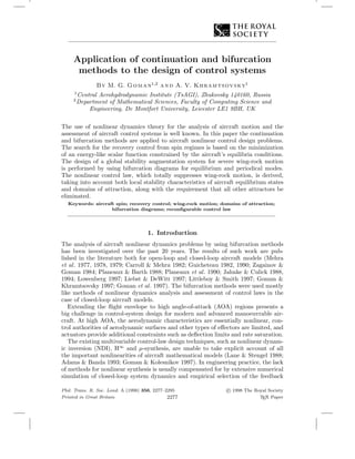
- 16. 2292 M. G. Goman and A. V. Khramtsovsky Figure 13. Domains of attraction for the closed-loop system at Kβ = 1.8, Kω = 9. Figure 14. Scheduling of feedback coefficients depending on the state variables—Kβ = 1.8, Kω = 9 if (p, β) ∈ S and Kβ = 0.2, Kω = 9 if (p, β) is out of S. point becomes stable; and the medium-sized closed orbit is close to vanishing. The region of attraction of the equilibrium point is composed of white areas (figure 12). At the fourth point with Kβ = 1.8 (see figure 13), there are only two attractors: a stable equilibrium (its domain of attraction is composed of white areas) and a large-sized closed orbit (the domain of attraction is filled by circles). Phil. Trans. R. Soc. Lond. A (1998)
- 17. Continuation and bifurcation methods for control system design 2293 Figure 15. Time histories of closed-loop system: (a) medium-sized oscillatory motion at Kβ = 1.0, Kω = 9; (b) large-sized oscillatory motion at Kβ = 1.0, Kω = 9; (c) feedback scheduling providing global stability for equilibrium flight Kβ = Kβ(p, β), Kω = 9. The medium-sized closed orbit from point (1) in the feedback plane (Kβ = 0.2, Kω = 9, see figure 10) is located totally inside the region of attraction S of the equilibrium state at point (4) in the feedback plane (Kβ = 1.8, Kω = 9, see figure 13). This is illustrated in figure 14. The information obtained during the qualitative analysis of closed-loop systems with different feedbacks enables the design of a variable-structure control law, which provides global stability for the equilibrium point. Inside the stability region S of the equilibrium point, corresponding to Kβ = 1.8, Kω = 9, the feedback coefficients are selected as point (4): Kβ = 1.8, Kω = 9 (see figure 14). This control will provide the convergence to the equilibrium point inside S. Outside region S, the feedback coefficients are to be changed to values from point Phil. Trans. R. Soc. Lond. A (1998)
- 18. 2294 M. G. Goman and A. V. Khramtsovsky (1): Kβ = 0.2, Kω = 9, providing the convergence to the stable, medium-sized, closed orbit, but it is totally located inside region S. Therefore, this variable-structure or reconfigurable control will provide stability for aircraft equilibrium flight and totally suppress all the periodical motion. Figure 15 shows time histories of the closed-loop system without scheduling at Kβ = 1.0, Kω = 9: (a) medium-sized limit cycle; (b) large-sized limit cycle; and (c) time history with the proposed scheduling of sideslip feedback coefficient Kβ(p, β) providing the global stability to aircraft equilibrium flight. 7. Conclusion The results presented demonstrate the efficiency of qualitative computational meth- ods of nonlinear dynamics analysis for the design of control laws, which prevent departures. They are especially important in cases where there is strong nonlinear behaviour due to nonlinearities in aerodynamics and the control system. This work was partly supported by a contract with the Defence Evaluation and Research Agency of Bedford, UK, and a Grant from the Russian Foundation for Basic Research N 96-01-00612. The authors are grateful to Dr Yoge Patel and Dr Darren Littleboy for valuable discussions. References Adams, R. J. & Banda, S. S. 1993 Robust flight control design using dynamic inversion and structured singular value synthesis. IEEE Trans. Control Syst. Tech. 1, 80–92. AGARD 1990 Rotary-balance testing for aircraft dynamics. AGARD Advisory Report no. 265. Carroll, J. V. & Mehra, R. K. 1982 Bifurcation analysis of nonlinear aircraft dynamics. J. Guidance 5, 529–536. Cobleigh, B. R., Croom, M. A. & Tamrat, B. F. 1994 Comparison of X-31 flight, wind-tunnel, and water-tunnel yawing moment asymmetries at high angles of attack. High Alpha Conference IY: Electronic Workshop, NASA Dryden Flight Research Center, 12–14 July 1994, Paper HA-AERO-06. URL: http://www.dfrf.nasa.gov/Workshop/HighAlphaIV/highalpha.html. Doedel, E. & Kernevez, J. P. 1986 AUTO: Software for continuation and bifurcation problems in ordinary differential equations. California Institute of Technology, Pasadena. Goman, M. G. 1986 Differential method for continuation of solutions to systems of finite nonlin- ear equations depending on a parameter. Uchenye zapiski TsAGI 17(5), 94–102. (In Russian.) Goman, M. & Khrabrov, A. 1994 State-space representation of aerodynamic characteristics of an aircraft at high angles of attack. J. Aircraft 31, 1109–1115. Goman, M. G. & Khramtsovsky, A. V. 1993 KRIT: Scientific package for continuation and bifurcation analysis with aircraft dynamics applications. TsAGI. Contract Report for DRA Bedford. Goman, M. G. & Khramtsovsky, A. V. 1997 Global stability analysis of nonlinear aircraft dynam- ics. AIAA Atmospheric Flight Mechanics Conf., New Orleans, LA, August, Paper 97-3721. Goman, M. G. & Kolesnikov, E. N. 1997 Robust control law design for an aircraft spatial motion. In Proc. Int. Symp. ‘Aviation 2000. Prospects’, Zhukovsky, Moscow Region, Russia, August 1997, pp. 147–158. Goman, M. G., Khramtsovsky, A. V. & Usoltsev, S. P. 1995 High incidence aerodynamics model for hypothetical aircraft. TsAGI Contract Report for DRA Bedford. Goman, M. G., Fedulova, E. V. & Khramtsovsky, A. V. 1996 Maximum stability region design for unstable aircraft with control constraints. AIAA Guidance Navigation and Control Con- ference, San Diego, CA, Paper N 96-3910. Goman, M. G., Zagainov, G. I. & Khramtsovsky, A. V. 1997 Application of bifurcation methods to nonlinear flight dynamics problems. J. Progr. Aero. Sci. 33, 539–586. Phil. Trans. R. Soc. Lond. A (1998)
- 19. Continuation and bifurcation methods for control system design 2295 Guicheteau, P. 1982 Bifurcation theory applied to the study of control losses on combat aircraft. Recherche Aerospatiale 2, 61–73. Guicheteau, P. 1990 Bifurcation theory in flight dynamics. An application to a real combat aircraft. ICAS Paper 116 (90-5.10.4). Guicheteau, P. 1992 Notice d’utilisation du code ASDOBI. Preprint ONERA. Jahnke, C. C. & Culick, F. E. C. 1988 Application of dynamical systems theory to nonlinear aircraft dynamics. AIAA Atmospheric Flight Mechanics Conf., Minneapolis, MN, August, AIAA Paper 88-4372. Jahnke, C. C. & Culick, F. E. C. 1994 Application of bifurcation theory to high-angle-of-attack dynamics of the F-14. J. Aircraft 31, 26–34. Lane, S. H. & Stengel, R. F. 1988 Flight control design using non-linear inverse dynamics. Automatica 24, 471–483. Liebst, B. S. & DeWitt, B. R. 1997 Wing rock suppression in the F-15 aircraft. AIAA Atmo- spheric Flight Mechanics Conf., New Orleans, LA, August, Paper 97-3719. Littleboy, D. M. & Smith, P. R. 1997 Bifurcation analysis of a high incidence aircraft with non- linear dynamic inversion control. AIAA Atmospheric Flight Mechanics Conf., New Orleans, LA, August, Paper 97-3717. Lowenberg, M. H. 1997 Bifurcation analysis as a tool for post-departure stability enhancement. AIAA Atmospheric Flight Mechanics Conf., New Orleans, LA, August, Paper 97-3716. Mehra, R. K., Kessel, W. C. & Carroll, J. V. 1977 Global stability and control analysis of aircraft at high angles of attack. Annual Technical Report 1, ONR-CR215-248-(1), Scientific Systems Inc., USA. Mehra, R. K., Kessel, W. C. & Carroll, J. V. 1978 Global stability and control analysis of aircraft at high angles of attack. Annual Technical Report 2, ONR-CR215-248-(2), Scientific Systems Inc., USA. Mehra, R. K., Kessel, W. C. & Carroll, J. V. 1979 Global stability and control analysis of aircraft at high angles of attack. Annual Technical Report 3, ONR-CR215-248-(3), Scientific Systems Inc., USA. Planeaux, J. B. & Barth, T. J. 1988 High angle of attack dynamic behavior of a model high performance fighter aircraft. AIAA Atmospheric Flight Mechanics Conf., Minneapolis, MN, August, AIAA Paper 88-4368. Planeaux, J. B., Beck, J. A. & Baumann, D. D. 1990 Bifurcation analysis of a model fighter aircraft with control augmentation. AIAA Atmospheric Flight Mechanics Conf., Portland, OR, August, AIAA Paper 90-2836. Tobak, M., Chapman, G. T. & Schiff, L. B. 1985 Mathematical modeling of the aerodynamic characteristics in flight mechanics. In Proc. of the Berkeley-Aimes Conf. on Nonlinear Prob- lems in Control and Fluid Dynamics, pp. 435–450. Brookline, MA: Math Science Press. (Also NASA TM-85880, January 1984.) Wood, E. F., Kempf, J. A. & Mehra, R. K. 1984 BISTAB: A portable bifurcation and stability analysis package. Appl. Math. Comp. 15. Zagainov, G. I. & Goman, M. G. 1984 Bifurcation analysis of critical aircraft flight regimes. Int. Council Aero. Sci. 84, 217–223. Phil. Trans. R. Soc. Lond. A (1998)